Detection and Localization for Multiple Stationary Human Targets Based on Cross-Correlation of Dual-Station SFCW Radars

Abstract

This paper demonstrates the feasibility of detection and localization of multiple stationary human targets based on cross-correlation of the dual-station stepped-frequency continuous-wave (SFCW) radars. Firstly, a cross-correlation operation is performed on the preprocessed pulse signals of two SFCW radars at different locations to obtain the correlation coefficient matrix. Then, the constant false alarm rate (CFAR) detection is applied to extract the ranges between each target and the two radars, respectively, from the correlation matrix. Finally, the locations of human targets is calculated with the triangulation localization algorithm. This cross-correlation operation mainly brings about two advantages. On the one hand, the cross-correlation explores the correlation feature of target respiratory signals, which can effectively detect all targets with different signal intensities, avoiding the missed detection of weak targets. On the other hand, the pairing of two ranges between each target and two radars is implemented simultaneously with the cross-correlation. Experimental results verify the effectiveness of this algorithm.

1. Introduction

As an emerging technology, ultra-wideband (UWB) radars are widely used in the field of life detection with the development of signal-processing technology. Especially in post-disaster rescue, anti-terrorism, and fall detection, the non-line-of-sight, long-range, and anti-interference characteristics make the radar an effective monitoring tool [1,2,3,4,5,6,7,8,9,10]. Therefore, it is of great practical significance to apply the radar to the detection and localization of human targets trapped behind obstructions.

A single-frequency continuous-wave radar was first utilized for contactless detection of human-respiration life signs in 1971 [11]. The Fourier transform is performed in [12,13] to extract respiration-frequency information from the radar signal with period micro-Doppler modulation. To obtain the range information of stationary human targets, UWB radars with a short pulse [14] and linear frequency-modulation continuous waves [15] were introduced for their high range resolution. Specifically, by performing Fourier transform along slow time, range information between radar and human target can be obtained, along with the extraction of respiration frequency. The stepped-frequency continuous-wave (SFCW) UWB radar has been the preferred choice in human detection due to its high sensitivity, flexible waveform controllability, and simple system design [16,17,18,19]. To further obtain accurate location information of human targets, multichannel UWB radar systems have increasingly been applied to human detection with two main methods. One extracts the target location from the target image formed by energy accumulation of multichannel target echoes [20]. The other first extracts a target range from the range Doppler (RD) plane that is formed by fast Fourier transform (FFT)-based energy accumulation of multiperiod echoes according to each transmit–receive channel, and then the target location is calculated by integrating two extracted target ranges of two channels [21]. However, these two methods have certain problems in the case of multiple human targets. First, since the two methods both depend on energy accumulation, weak target are masked by targets with strong echo intensity, resulting in missed detections of weak targets. The difference of echo intensity may frequently be encountered in practice due to, for example, different target ranges or intertarget occlusion. Second, for the second method in [21] with two transmit–receive channels, multiple target ranges are acquired in each channel, thus an additional pairing procedure is required to sort out two-channel ranges of each target. More seriously, false targets appear accompanied with the inevitable false pairing for some specific target locations.

To avoid the missed detection of weak targets, a single-radar correlation-based method is proposed in [22] to substitute the energy accumulation-based method. Based on a single-channel UWB pulse radar, the correlation coefficient of multiperiod echoes of each target is explored to identify the range information of all targets with different echo intensity. Nevertheless, this method is only able to obtain ranges (rather than locations) of multiple stationary human targets due to single-channel processing. Even if this method is introduced into multichannel radars, namely the correlation operation is performed on each channel, the pairing of extracted target ranges of a multichannel is also indispensable for subsequent target localization. Furthermore, a weak target also disappears under the condition of serious intertarget occlusion. With respect to a single-station one-transmitter and two-receiver (two-channel) SFCW radar, interchannel cross-correlation was considered to improve the detection performance in low signal-to-noise ratio (SNR) backgrounds [23]. Cross-correlation is implemented by multiplying two-channel RD planes; in essence, it is also based on energy accumulation. Moreover, in two RD planes, a necessary but uncommon condition for a multiplication operation is that each target should be located in the same RD cells.

In this paper, a cross-correlation algorithm based on dual-station single-channel SFCW radars is proposed to implement the detection and localization of multiple stationary human targets. With regard to two single-channel radars at different stations, the respiration signals of each target in two different channels are highly related, so the cross-correlation coefficient matrix of two-channel echoes is first calculated as the basis of subsequent target detection. In particular, target detection is performed on the cross-correlation coefficient matrix by a two-dimension constant false alarm rate (CFAR) detector to achieve the ranges of multiple targets [24]. Finally, the triangulation method is utilized to convert the extracted target ranges to the estimations of target locations. The main contributions are as follows:

1. Dual-view synchronous observation is implemented by utilizing two single-channel SFCW radars at different stations, which brings about two major advantages. On the one hand, intertarget shadowing occlusion (generally appeared in the case of single-view observation) is widely prevented to ensure robust detection of multiple stationary human targets. On the other hand, favorable adaptability is achieved for different radar locations and human-target orientations.

2. Compared with existent energy-accumulation algorithms [19,20,23] and the single-radar correlation algorithm [22], the proposed cross-correlation algorithm of dual-station radars efficiently deals with the problem of the missed detection of weak targets even in the case of target occlusion for one of two radars.

3. In comparison to the two-channel processing algorithm [21] and single-radar correlation algorithm [22], the proposed cross-correlation algorithm dispenses with the additional-range pairing procedure, as two extracted ranges of each target for two radars are synchronously connected in the cross-correlation process.

Based on two SFCW radar at different stations, multiple groups of experiments were carried out to validate the superiority of the proposed cross-correlation algorithm in comparison to the energy-accumulation and single-channel correlation algorithms, and evaluate the performance with different radar locations, human-target orientations, and postures.

The paper is organized as follows. Section 2 introduces the configuration of dual-station SFCW radars. The principle of proposed cross-correlation algorithm is described in Section 3. In Section 4, the experiment results and analyses are presented. The paper is concluded in Section 5.

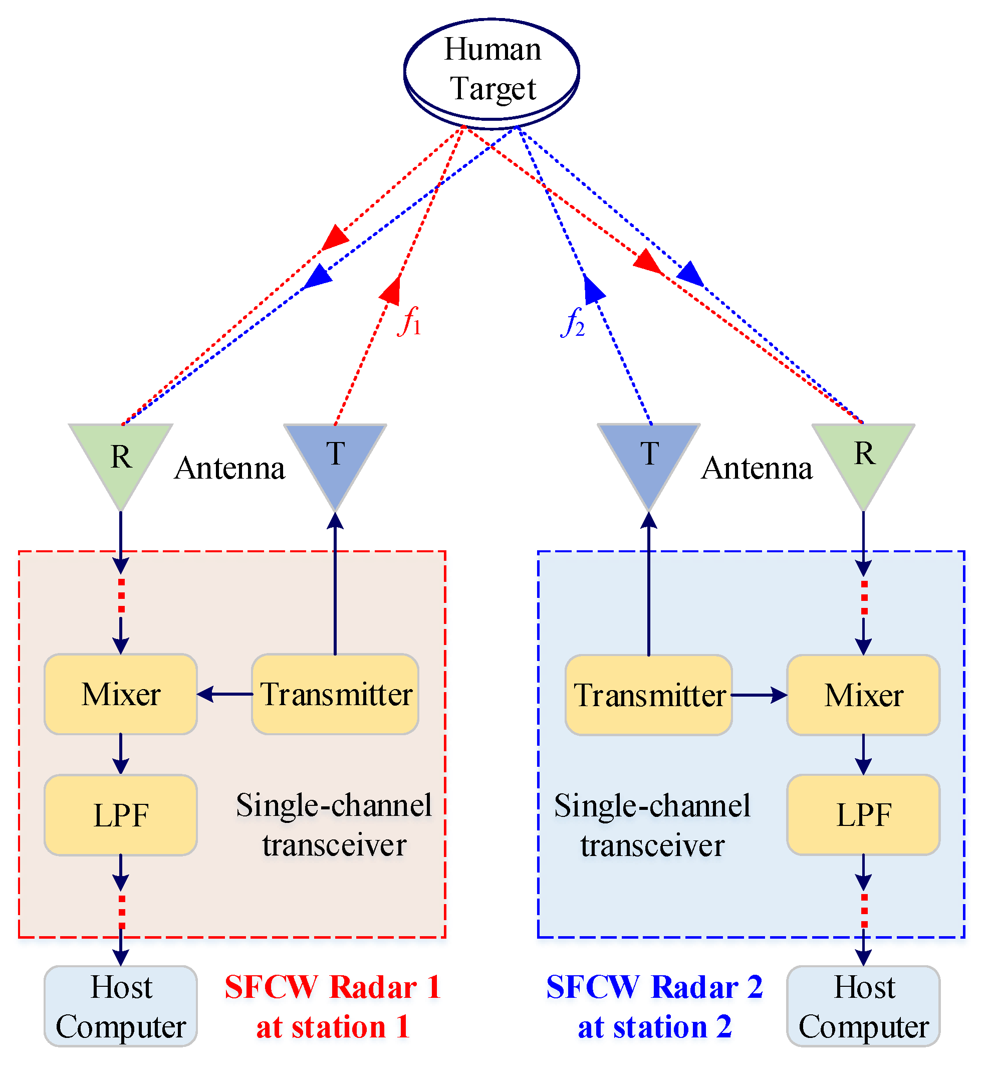
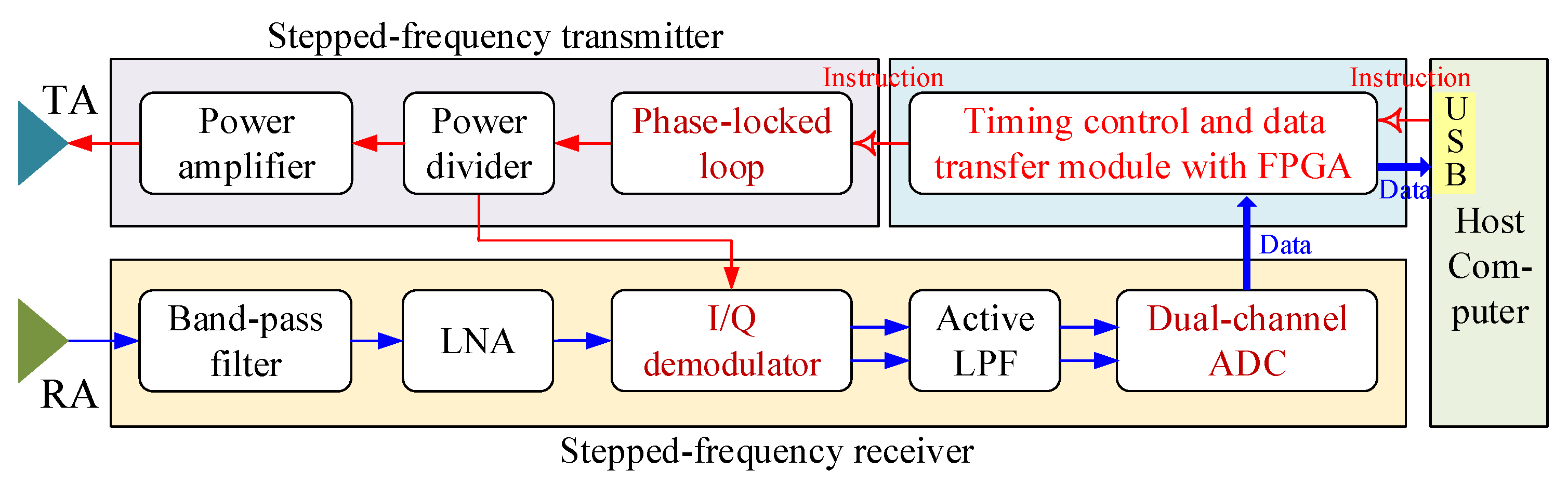
2. Dual-Station SFCW Radar

The dual-station radar system consists of two single-channel SFCW radars located at different locations, as shown in Figure 1. The detailed radar structure is provided in Section 4. Each SFCW radar is composed of three parts: host computer, single-channel transceiver, and two antennas. The host computer plays the role of displaying and controlling the terminal, which manages operation parameters, and the storage and presentation of collected data. The single-channel transceiver is responsible for the generation, transmission, reception, and sampling of SFCW signals. The two antennas are connected to the single-channel transceiver for the radiation of electromagnetic waves and collection of target echoes.

The application of a SFCW signal can help avoid the mutual interference of two single-channel radars. This anti-interference ability can be interpreted as follows. The SFCW signal involves a sequence of discrete tones whose carrier frequencies are increased by a fixed stepwise manner to cover a wide bandwidth in the time domain. Therefore, the SFCW signal can be expressed as

$$\begin{array}{c}\hfill s\left(t\right)=\sum _{k=0}^{K}cos\left(2\pi (f_0+k\Delta f)t\right)·rect\left(\frac{t-k{T}_0-\frac{1}{2}{T}_0}{T_0}\right),\end{array}$$

(1)

where $f_0$ is the starting carrier frequency, $\Delta f$ is the frequency increment, $T_0$ is the duration time of each frequency, and $K+1$ is the number of all carrier frequencies. To decrease pulse-repetition time, single-frequency time $T_0$ is generally limited to the microsecond level. In this paper, the $T_0$ of the developed single-channel radar is configured as 100 μs. Obviously, the same carrier frequency electromagnetic wave emitted from the two radars at the same time causes mutual interference between the radars. To prevent this interference in practical applications, two single-channel radars at different locations are set up to perform asynchronous observations by manual activation from corresponding host computers. Manual activation inevitably results in millisecond levels of minor observation-time differences for the two single-channel radars. For the millisecond-level single-frequency time, the minor time difference brings about a significant distinction between the working carrier frequencies of two radars. Specifically, we assume Radar 1 runs at a carrier frequency of $f_1$ while Radar 2 works in $f_2$ at the same time. In this case, two radars simultaneously receive target echoes with $f_1$ and $f_2$. Take the case of Radar 1. The target echo of $f_2$ is regarded as interference from Radar 2. The target echoes of $f_1$ and $f_2$ are demodulated separately in the mixer with a carrier frequency of $f_1$, correspondingly generating the desired baseband signal and the interference signal with a frequency of $|f_1-f_2|$. By a low-pass filter (LPF), the desired baseband signal of Radar 1 is preserved to serve for human detection, and the interference signal from Radar 2 is filtered out. In the same way, the interference signal from Radar 1 could be removed in Radar 2 through demodulation and filtering. In terms of human-target detection, the millisecond time difference is negligible for several (3–4) seconds of human respiration, guaranteeing the high correlation of respiration signals between two radars for each human target. As a whole, the application of the SFCW system enables effective observation of two radars without mutual interference.

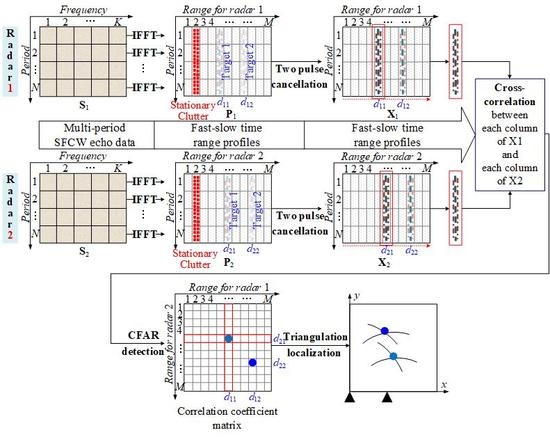
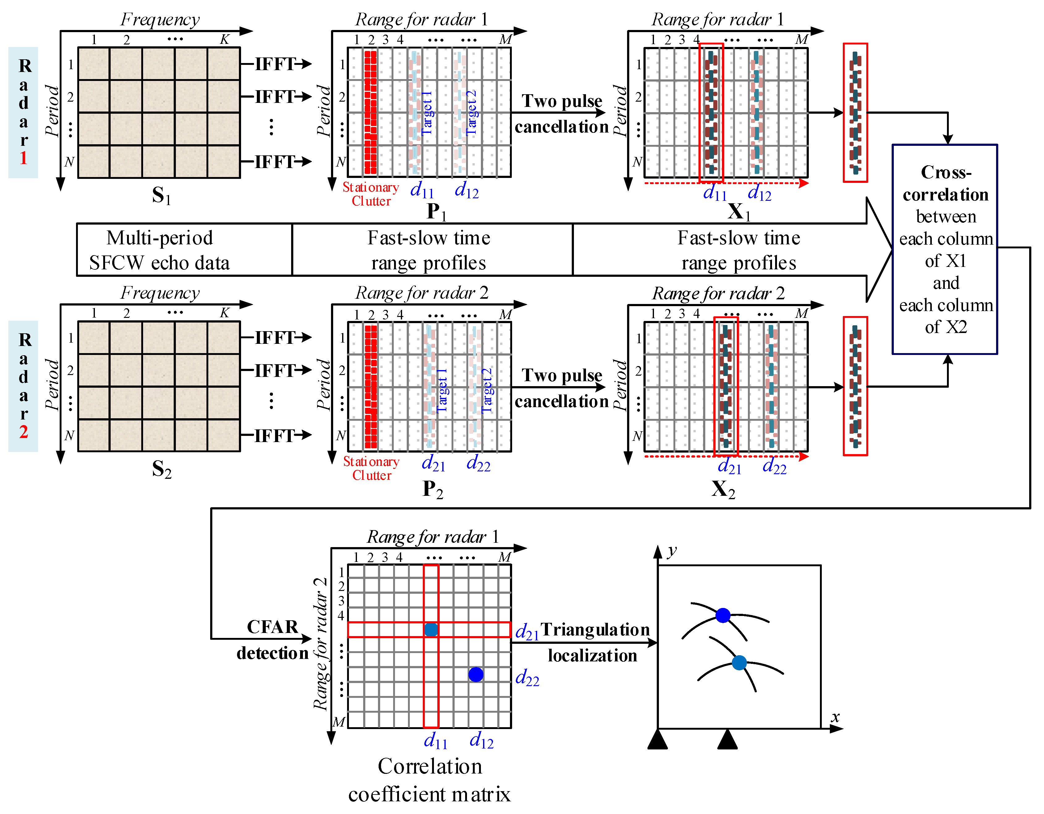
3. Dual-Station Cross-Correlation Based Detection and Localization

In this section, a dual-station cross-correlation algorithm is presented to implement the detection and localization of multiple stationary human targets. As shown in Figure 2, with respect to the multiperiod SFCW echo data of two radars, the presented algorithm is composed of five steps: inverse FFT (IFFT) for generating range profiles, two-pulse cancellation for suppressing stationary background clutters, cross-correlation between two radars for exploring the correlation feature of respiratory signals, CFAR detection for identifying multiple targets, and triangulation localization for calculating target locations. A detailed description of these steps is provided as follows.

3.1. Signal Model

With respect to stationary human detection, the desired characteristics are nonstationary and quasiperiodic fluctuations of a body surface caused by respiration and heartbeat. However, in real application situations, heartbeat fluctuations are too weak to be detected due to medium penetration attenuation. Therefore, excluding heartbeat fluctuations, the nonstationary and quasiperiodic fluctuations of a body surface only with respiration is approximately modeled into a narrow-band random signal as

$$\Delta r\left(t\right)=A_b\left(t\right)sin({\omega }_b\left(t\right)t+{\phi }_b\left(t\right)),$$

(2)

where $A_b\left(t\right)$, ${\omega }_b\left(t\right)$, and ${\phi }_b\left(t\right)$ denote respiration amplitude, frequency, and initial phase with slow random variation, respectively.

To extract the quasiperiodic micromotion respiration signal, it is necessary to collect multiple periods of SFCW echoes. More echo periods mean higher SNR and better frequency resolution, but result in a larger processing burden and delay. As for the selection of period number, a trade-off must be made to satisfy the practical application demand. Assume there are $\beta$ stationary human targets and N periods of SFCW echoes collected for each radar. For each period, through quadrature demodulation, multipoint sampling and averaging in each frequency, a sequence of multifrequency echo data are acquired as a frequency-domain data vector. Assume that there are totally $K+1$ frequencies. Therefore, N periods of data vectors are combined into a $N\times K+1$ data matrix ${\mathbf{S}}_l$, where the nth row and kth column of an element can be given by

$$\begin{array}{c}\hfill {\mathbf{S}}_l(n,k)=\sum _{\lambda =1}^{\beta }exp\left(-j2\pi (f_0+k\Delta f)\left(\frac{{\overline{r}}_{l,\lambda }+\Delta r_l\left(t_{n,\lambda }\right)}{c}\right)\right),\end{array}$$

(3)

where $l=$ 1 and 2 are used to classify Radars 1 and 2, ${\overline{r}}_{l,\lambda }$ is the average range between radar l and torso surface of $\lambda$th human target, c is the light speed, and $\Delta r_l\left(t_{n,\lambda }\right)$ is the range fluctuation regarded as an invariant for all $K+1$ frequencies in the nth period.

3.2. Data Preprocessing

For multiperiod multifrequency data matrix ${\mathbf{S}}_l$, to obtain narrow pulse signals with target ranges, IFFT-based pulse compression is performed on each period of a multifrequency data vector to generate a period of the time-domain range profile. For example, the nth period of the range profile can be written as

$$\begin{array}{c}\hfill p_l(n,r_m)=\sum _{\lambda =1}^{\beta }B·\mathrm{sinc}\left(B\left(r_m-2({\overline{r}}_{l,\lambda }+\Delta r_l\left(t_{n,\lambda }\right))\right)\right)·exp\left(j2\pi f_c\left(r_m-2({\overline{r}}_{l,\lambda }+\Delta r_l\left(t_{n,\lambda }\right))\right)\right),\end{array}$$

(4)

where $B=K\Delta f$ and $f_c=f_0+K\Delta f/2$ separately denote the bandwidth and center frequency of SFCW signal, and $r_m$ is the mth computational range unit. Maximum unambiguous range $c/2\Delta f$ is divided into M computational range units through M points of IFFT. To accurately track the target peak, the point number of IFFT, namely, the number of computational range units is generally set to be larger than the number of physical range units, namely $M>K$. In other words, the echo of one target extends to multiple computational range units.

With regard to the N periods of SFCW echoes for radar $l(l=1,2)$, N periods of range profiles are generated through IFFT on each period, forming an $N\times M$ dimension of fast–slow time data matrix ${\mathbf{P}}_l$. Considering that practical life detection situations are full of strong stationary clutters (such as ground, wall, and debris echoes) and background noise, the complete fast–slow time data matrix ${\mathbf{P}}_l$ can be expressed as

$${\mathbf{P}}_l={\mathbf{P}}_{h,l}+{\mathbf{P}}_{w,l}+{\mathbf{\omega }}_{n,l},$$

(5)

where ${\mathbf{P}}_{h,l}$ expresses the desired human signals, ${\mathbf{P}}_{w,l}$ represents the stationary clutters, ${\mathit{\omega }}_{n,l}$ denotes the background noise, and $l=$ 1 and 2 are used to classify Radars 1 and 2. As a result, fast–slow time data matrices ${\mathbf{P}}_1$ and ${\mathbf{P}}_2$ are obtained through IFFT on each period of two multi-frequency data matrices ${\mathbf{S}}_1$ and ${\mathbf{S}}_1$ separately collected by Radar 1 and Radar 2.

For these two fast–slow time matrices ${\mathbf{P}}_1$ and ${\mathbf{P}}_2$, preprocessing is required to suppress the stationary clutters in each matrix before cross-correlation operation. In this section, two instances of pulse-cancellation filtering are utilized to reduce stationary clutters as

$$\begin{array}{c}{\mathbf{X}}_1(n,m)={\mathbf{P}}_1(n,m)-{\mathbf{P}}_1(n+1,m)\hfill \\ {\mathbf{X}}_2(n,m)={\mathbf{P}}_2(n,m)-{\mathbf{P}}_2(n+1,m),\hfill \end{array}$$

(6)

where n and m indicate the index of the matrix row (period) and column (computational range unit), respectively. The values of n and m are $n=1,2,\cdots ,N-1$ and $m=1,2,\cdots ,M$.

It should be noticed that, in [22], the average cancellation method is utilized for clutter suppression. This method can effectively suppress the stationary clutter while preserving the integrity of the target signal. However, due to the characteristic of SFCW pulse compression, the target signal is always accompanied by a large number of side lobes. If the average cancellation is utilized, most of these side lobes would be retained. These retained side lobes would cause large areas of high correlation to appear as ghost interference in the results of cross-correlation operations. For this reason, two instances of pulse cancellation are utilized in this paper for clutter suppression because side lobes could be decreased to be submerged with the noise, although a part of the target signal is simultaneously suppressed.

3.3. Dual-Station Cross-Correlation

With regard to either matrix ${\mathbf{X}}_1$ or ${\mathbf{X}}_2$ after clutter cancellation, the existent method based on energy accumulation performs FFT on each column of computational range unit along slow time dimension to obtain the RD plane. Because the amplitude of respiration, micromotion is too small, the weak respiration signals disperse to all periods across slow time in target range units, which are accumulated to improve SNR for robustly extracting respiration frequency and range of human target. However, in the case of multiple human targets, the FFT-based method suffers from two fatal problems, namely, missed detections of weak targets, and pairing two extracted ranges of each target between two radars (for subsequent target localization). To deal with these two problems, the proposed algorithm revolves around dual-station cross-correlation of respiration life signals rather than FFT accumulation to implement the detection and localization of multiple stationary human targets.

Based on the experiment results, it could be found that, for the same target, the slow time respiration signals in target range units had similarity between the two radars at different stations. Therefore, dual-station cross-correlation is proposed to explore the similarity for the purpose of detection and localization of multiple human targets. Let ${\mathit{x}}_{1i}$ and ${\mathit{x}}_{2i^{\prime }}$ denote the sampling data of slow time at computational range units of one target, namely, the ith and $i^{\prime }$th column of data in ${\mathbf{X}}_1$ and ${\mathbf{X}}_2$, which can be expressed as

$$\left\{\begin{array}{c}{\mathit{x}}_{1i}={\mathit{s}}_{1i}+{\mathit{n}}_{1i}\\ {\mathit{x}}_{2i^{\prime }}={\mathit{s}}_{2i^{\prime }}+{\mathit{n}}_{2i^{\prime }},\end{array}\right.$$

(7)

where ${\mathit{s}}_{1i}$ and ${\mathit{s}}_{2i^{\prime }}$ are the respiration signals corresponding to the two radars, respectively, and ${\mathit{n}}_{1i}$ and ${\mathit{n}}_{2i^{\prime }}$ represent the background noise. The cross-correlation coefficient $r_{{\mathit{x}}_{1i}{\mathit{x}}_{2i^{\prime }}}$ of ${\mathit{x}}_{1i}$ and ${\mathit{x}}_{2i^{\prime }}$ can be calculated as

$$\begin{array}{cc}{r}_{{\mathit{x}}_{1i}{\mathit{x}}_{2i^{\prime }}}\hfill & =\frac{\mathrm{cov}({\mathit{x}}_{1i},{\mathit{x}}_{2i^{\prime }})}{\sqrt{\mathrm{D}\left({\mathit{x}}_{1i}\right)}\sqrt{\mathrm{D}\left({\mathit{x}}_{2i^{\prime }}\right)}}\hfill \\ & =\frac{\mathrm{E}\left(\left[{\mathit{x}}_{1i}-\mathrm{E}\left({\mathit{x}}_{1i}\right)\right]\left[{\mathit{x}}_{2i^{\prime }}-\mathrm{E}\left({\mathit{x}}_{2i^{\prime }}\right)\right]\right)}{\sqrt{\mathrm{E}\left({\left[{\mathit{x}}_{1i}-\mathrm{E}\left({\mathit{x}}_{1i}\right)\right]}^2\right)}\sqrt{\mathrm{E}\left({\left[{\mathit{x}}_{2i^{\prime }}-\mathrm{E}\left({\mathit{x}}_{2i^{\prime }}\right)\right]}^2\right)}},\hfill \end{array}$$

(8)

where $\mathrm{cov}\left(\right)$ represents covariance calculation, $\mathrm{E}\left(\right)$ is statistical averaging, and $\mathrm{D}\left(\right)$ denotes variance computation.

Since the background noises of the two radars are not only independent from each other, but also uncorrelated with the respiration signals, $r_{{\mathit{x}}_{1i}{\mathit{x}}_{2i^{\prime }}}$ can be expressed as

$$r_{{\mathit{x}}_{1i}{\mathit{x}}_{2i^{\prime }}}=\frac{\mathrm{cov}({\mathit{s}}_{1i},{\mathit{s}}_{2i^{\prime }})}{\sqrt{\mathrm{D}\left({\mathit{s}}_{1i}\right)}\sqrt{\mathrm{D}\left({\mathit{s}}_{2i^{\prime }}\right)}}=r_{{\mathit{s}}_{1i}{\mathit{s}}_{2i^{\prime }}}.$$

(9)

It can be perceived from Equation (9) that, between these two sets of slow-time sampling data ${\mathit{x}}_{1i}$ and ${\mathit{x}}_{2i^{\prime }}$ in the target range units of two radars, cross-correlation coefficient $r_{{\mathit{x}}_{1i}{\mathit{x}}_{2i^{\prime }}}$ is mainly determined by the desired respiration signals rather than the noise. Because of the similarity between the respiration signals of the two radars, the cross-correlation coefficient is close to 1. On the contrary, due to irrelevance between two targets or between target and noise, in the corresponding range units, the cross-correlation coefficient of slow-time sampling data approaches 0. It can be seen that the irrelevance of two human targets results from the independent random feature of nonstationary and quasiperiodic respiration signals of different targets. Therefore, this correlation characteristic could be utilized to classify and detect different targets.

To explore the correlation feature, with respect to fast–slow time data matrices ${\mathbf{X}}_1$ and ${\mathbf{X}}_2$, we perform a cross-correlation operation for each column of ${\mathbf{X}}_1$ with each column of ${\mathbf{X}}_2$ to calculate the cross-correlation coefficient as

$$\begin{array}{c}\hfill \mathbf{R}\left(i,i^{\prime }\right)=\frac{\left|{\sum }_{n=1}^N\left({\mathit{x}}_{1i}\left(n\right)-{\overline{\mathit{x}}}_{1i}\right)\left({\mathit{x}}_{2i^{\prime }}\left(n\right)-{\overline{\mathit{x}}}_{2i^{\prime }}\right)\right|}{\sqrt{{\sum }_{n=1}^N{\left({\mathit{x}}_{1i}\left(n\right)-{\overline{\mathit{x}}}_{1i}\right)}^2}\sqrt{{\sum }_{n=1}^N{\left({\mathit{x}}_{2i^{\prime }}\left(n\right)-{\overline{\mathit{x}}}_{2i^{\prime }}\right)}^2}},\end{array}$$

(10)

where ${\mathit{x}}_{1i}\left(n\right)$ denotes the nth data element in the ith column of ${\mathbf{X}}_1$, ${\mathit{x}}_{2i^{\prime }}\left(n\right)$ represents the nth data element in the $i^{\prime }$th column of ${\mathbf{X}}_2$, and ${\overline{\mathit{x}}}_{1i}$, and ${\overline{\mathit{x}}}_{2i^{\prime }}$ are the averaging of ith column of data in ${\mathbf{X}}_1$ and $i^{\prime }$th column of data in ${\mathbf{X}}_2$, separately. After the correlation calculation for all data columns of ${\mathbf{X}}_1$ and ${\mathbf{X}}_1$, an $M\times M$ dimension of correlation coefficient matrix $\mathbf{R}$ is generated, where $\mathbf{R}(i,i^{\prime })$ is the element in ith row and $i^{\prime }$th column standing for the correlation degree between the ith data column of ${\mathbf{X}}_1$ and the $i^{\prime }$th data column of ${\mathbf{X}}_2$. It is important to point out that the indices of the row and column of the coefficient matrix represent the range information by reference to Radars 1 and 2, respectively.

According to the aforementioned analysis on correlation characteristics, in correlation coefficient matrix $\mathbf{R}$, different targets are isolated and focused on different elements. For the focused element of each target, the indices of the corresponding row and column denote the ranges from the target to Radar 1 and Radar 2, separately. Therefore, when the targets are detected in correlation coefficient matrix $\mathbf{R}$, two ranges between each target and the two radars are extracted simultaneously without additional pairing.

3.4. Target Identification and Localization

In this section, the CFAR detector is utilized to identify the stationary targets in correlation coefficient matrix $\mathbf{R}$. CFAR detection is an effective automatic-detection method that calculates the threshold corresponding to each element of the matrix $\mathbf{R}$ according to the deployed false alarm probability $P_{fa}$. The basic formula for calculating the threshold is given by

$$\tau =({P_{fa}}^{-1/N_c}-1)\sum _{n=1}^{N_c}\mathbf{R}\left(n\right),$$

(11)

where $N_c$ and $\mathbf{R}\left(n\right)$ denote the number and value of reference elements. The protection elements are selected to be excluded from the threshold calculation, avoiding nearby interference. With regard to two-dimensional correlation matrix $\mathbf{R}$, a sliding rectangular window is used to facilitate the detection process. The rectangular window with $L_c\times L_c$ (length × width) elements is centered at the element to be detected, which is divided into three parts: the centered detection element, reference elements, and protection elements. The protection elements are included in another smaller $L_g\times L_g$ concentric window. In this case, the number of reference elements and protection elements can be expressed separately as

$$\begin{array}{c}{N}_g={L_g}^2-1\hfill \\ N_c={L_c}^2-{L_g}^2.\hfill \end{array}$$

(12)

Consequently, for element $\mathbf{R}(i,i^{\prime })$ to be detected in ith row and $i^{\prime }$th column of matrix $\mathbf{R}$, the corresponding threshold $\tau (i,i^{\prime })$ can be calculated as

$$\begin{array}{c}\hfill \tau (i,i^{\prime })=({P_{fa}}^{-1/N_c}-1)\sum _{p=i-L_{ct}}^{i+L_{ct}}\sum _{q=i^{\prime }-L_{ct}}^{i^{\prime }+L_{ct}}\mathbf{R}\left(p,q\right)-({P_{fa}}^{-1/N_c}-1)\sum _{p=i-L_{gt}}^{i+L_{gt}}\sum _{q=i^{\prime }-L_{gt}}^{i^{\prime }+L_{gt}}\mathbf{R}\left(p,q\right),\end{array}$$

(13)

where $L_{ct}=(L_c-1)/2$ and $L_{gt}=(L_g-1)/2$. According to adaptive threshold $\tau (i,i^{\prime })$, element $\mathbf{R}(i,i^{\prime })$ to be detected is reassigned to 1 or 0 by the judgment criteria as

$$\mathbf{R}(i,i^{\prime })=\left\{\begin{array}{c}\begin{array}{cc}1,& \mathbf{R}(i,i^{\prime })>\tau (i,i^{\prime })\end{array}\\ \begin{array}{cc}0,& \mathbf{R}(i,i^{\prime })\le \tau (i,i^{\prime })\end{array}\end{array}\right..$$

(14)

Through the detection of each element as Equation (14), a detection output binary matrix $\mathbf{R}$ is obtained where 1 and 0 represented target existence and absence, respectively. In practical applications, because the respiration signal of each target extends to multiple computational range units in each period, each target takes up a connected region including a group of conterminous elements with a value of 1 in binary matrix $\mathbf{R}$. In the connected region, the centroid element is selected as representation whose indices of the corresponding row and column are translated into two ranges of a target from the two radars.

To obtain the target location from these two ranges, a coordinate system is established where the location of Radar 1 is taken as the origin, and the connection line of Radars 1 and 2 is regarded as the x-axis. In this case, the coordinates of Radars 1 and 2 are (0, 0) and $(d_r,0)$, where $d_r$ is the distance between these two radars. Assuming the extracted target ranges from the two radars are $d_1$ and $d_2$, estimation $(x_0,y_0)$ of the target location can be calculated by using the triangulation algorithm as

$$\left\{\begin{array}{c}{x}_0={\displaystyle \frac{{d_1}^2-{d_2}^2+{d_r}^2}{2d_r}}\\ y_0=\sqrt{{d_1}^2-{x_0}^2}\end{array}\right..$$

(15)

Under the condition of penetration detection, such as wall penetration, the estimated target location is displaced from the real target location due to the penetration decline of propagation velocity. For the purpose of correcting the displacement, assuming that the electromagnetic waves vertically propagate in the wall, the approximate compensation of wall penetration is performed as presented in [6] to modify the extracted target ranges from two radars. Specifically, with the prior information of wall thickness $d_w$ and relative permittivity ${ϵ}_w$, target ranges $d_1$ and $d_2$ are modified as

$$\begin{array}{c}{d_1}^{\prime }=d_1-2d_w\left(\sqrt{{ϵ}_w}-1\right)\hfill \\ {d_2}^{\prime }=d_2-2d_w\left(\sqrt{{ϵ}_w}-1\right).\hfill \end{array}$$

(16)

By substituting ${d_1}^{\prime }$ and ${d_2}^{\prime }$ for $d_1$ and $d_2$ in Equation (15), we can obtain a better estimation of target location with smaller displacement in comparison to that without wall compensation.

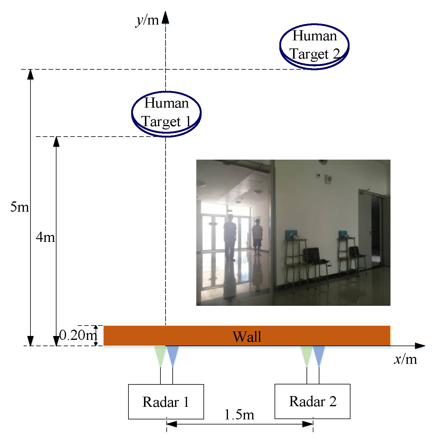
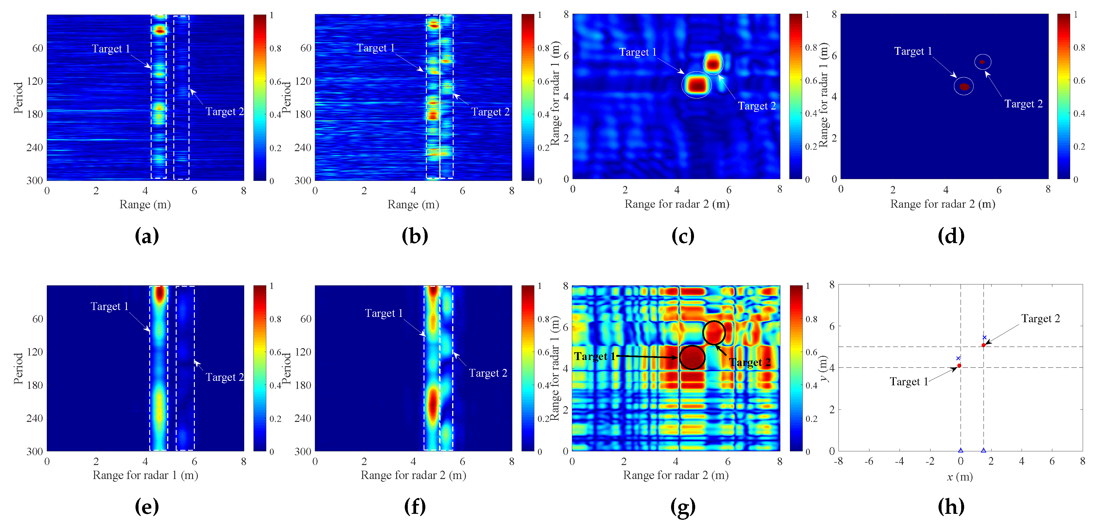
4. Experimental Results and Discussion

Two single-channel SFCW radars were fabricated to verify the capability of the proposed algorithm. Specifically, four groups of experiments were carried out in two different realistic scenarios. The radar description and experiment results are provided below in this section.

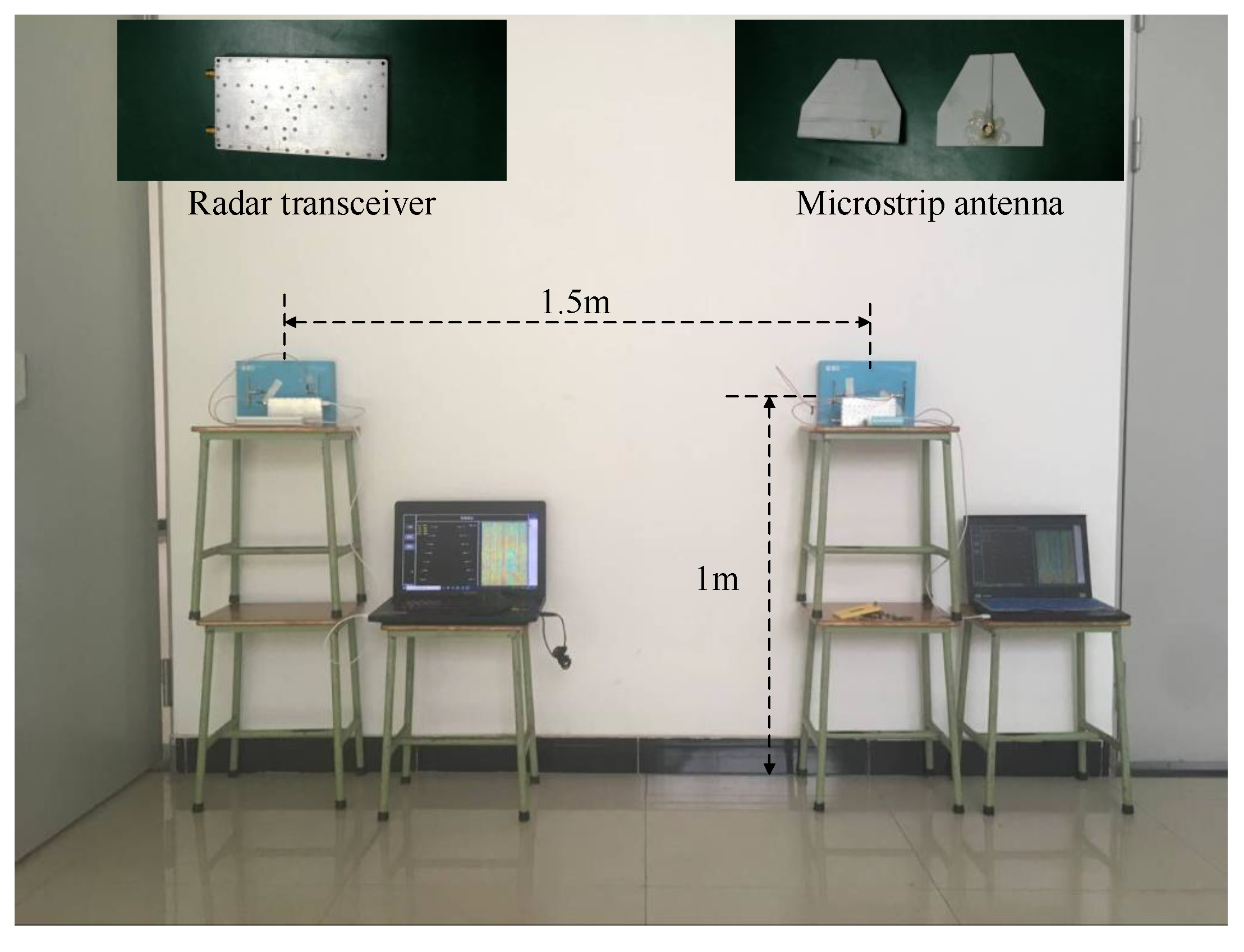
4.1. Description of Single-Channel SFCW Radar

The block diagram of the proposed single-channel SFCW radar is shown in Figure 3. It is clear that the radar system is composed of five key components: two transmitting/receiving antennas (TA/RA), a stepped-frequency (SF) transmitter, an SF receiver, an FPGA-based control transfer module, and a host computer with a user-friendly interface. In the process of signal generating, based on the activation instruction from the computer, the FPGA-based module controls the phase-locked loop within the SF transmitter to continuously generate a sequence of carrier frequencies with a fixed stepwise manner. Then, the carrier frequencies are divided into two channels through a power divider where the one is amplified to the TA and the other is transported to the I/Q quadrature demodulator as a reference signal. In the process of data acquisition, the reflected signals collected by the RA are filtered and amplified successively by a band-pass filter and a low-noise amplifier (LNA), and then the I/Q demodulator performs the coherent demodulation with use of the reference signal. Through the active LPF, the demodulated I/Q signals are filtered and amplified to produce the baseband I/Q signals, which are then sampled by utilizing a two-channel analog-to-digital converter (ADC). In the FPGA-based module, multiple sampled I-channel (Q-channel) data of each frequency are combined into an efficient I-channel (Q-channel) data by the averaging operation. Finally, through the USB port, the efficient I/Q data are serially transferred to the computer for storage and subsequent processing. The detailed parameters of the radar system are listed in

Table 1. The key parameters of SFCW radar.

Parameters	Value
Frequency number	301
Starting frequency	1.6 GHz
Ending frequency	2.2 GHz
Frequency step	2 MHz
Duration time of each frequency	100 μs
Bandwidth	600 MHz
Pulse repetition interval	30.1 ms
Radiation power	18 dBm
Sampling rate of ADC	250 KHz
Sampling bit number of ADC	14 bits

. These antennas are known as microstrip antennas whose parameters are given in

Table 2. The key parameters of microstrip antennas.

Parameters	Value
3 dB beamwidth in azimuth at 1.9 GHz (E plane)	$\pm {46}^{\circ }$
3 dB beamwidth in elevation at 1.9 GHz (H plane)	$\pm {30}^{\circ }$
Gain	>4 dB
Voltage standing wave ratio	<2
Size: maximum width	75 mm
Size: height	47 mm
Size: thickness	3 mm

. In all experiments outlined below, the distance between TA and RA was 0.1 m. For convenience, this distance was ignored in target localization.

Based on the operation parameters in Table 1, the maximum unambiguous range is 75 m and the range resolution is 0.25 m. Moreover, the data rate of each radar is about 35 KBps. Specifically, in the duration time of 100 μs of each frequency, there are totally two efficient data points for I/Q two channels. Each data point is represented by 14-bit binary numbers. Therefore, the data rate can be calculated as $\left(\left(2\times 14\mathrm{bit}\right)/100\mathsf{\mu }\mathrm{s}\right)/8=35\mathrm{KBps}$.

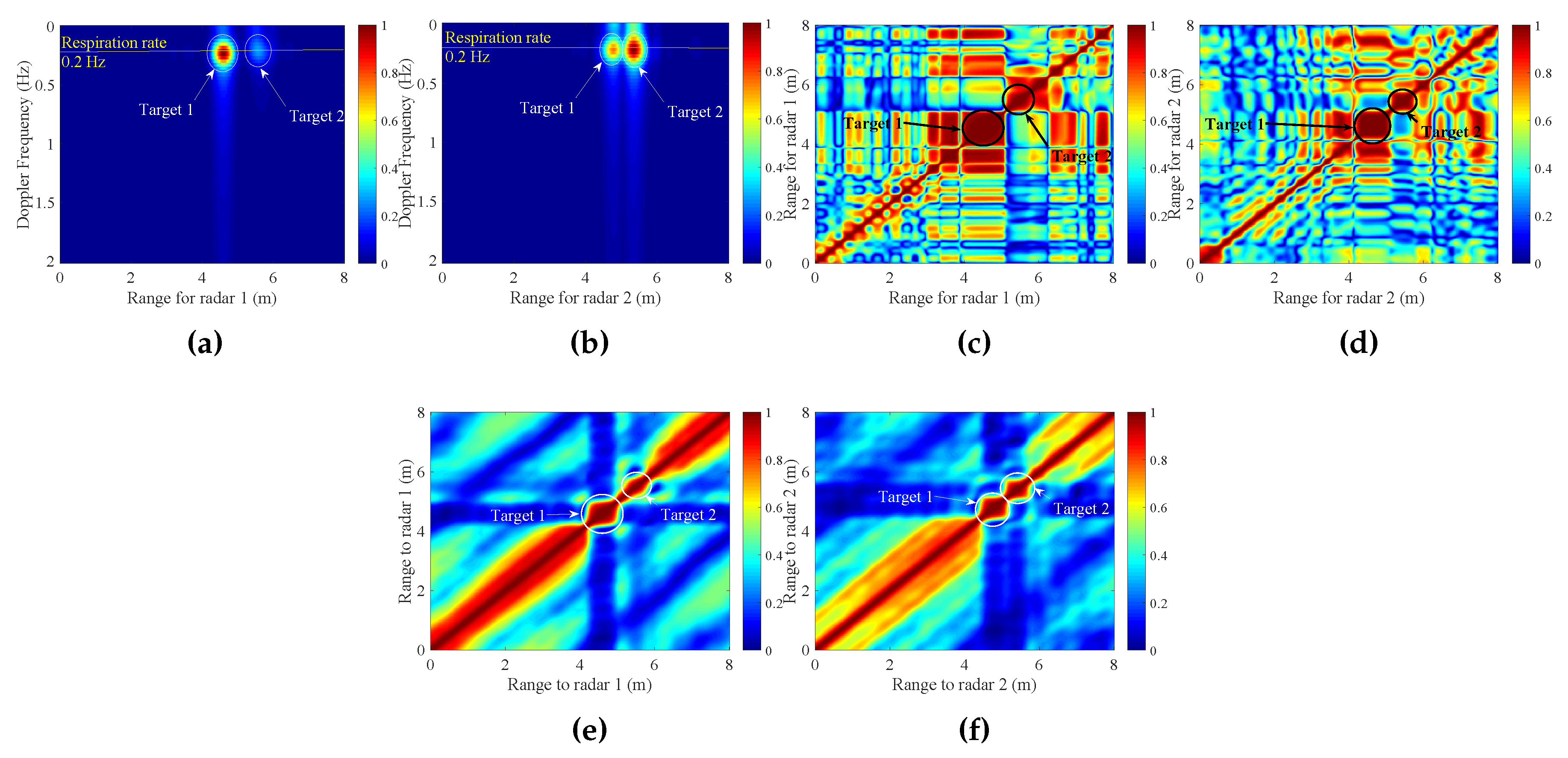
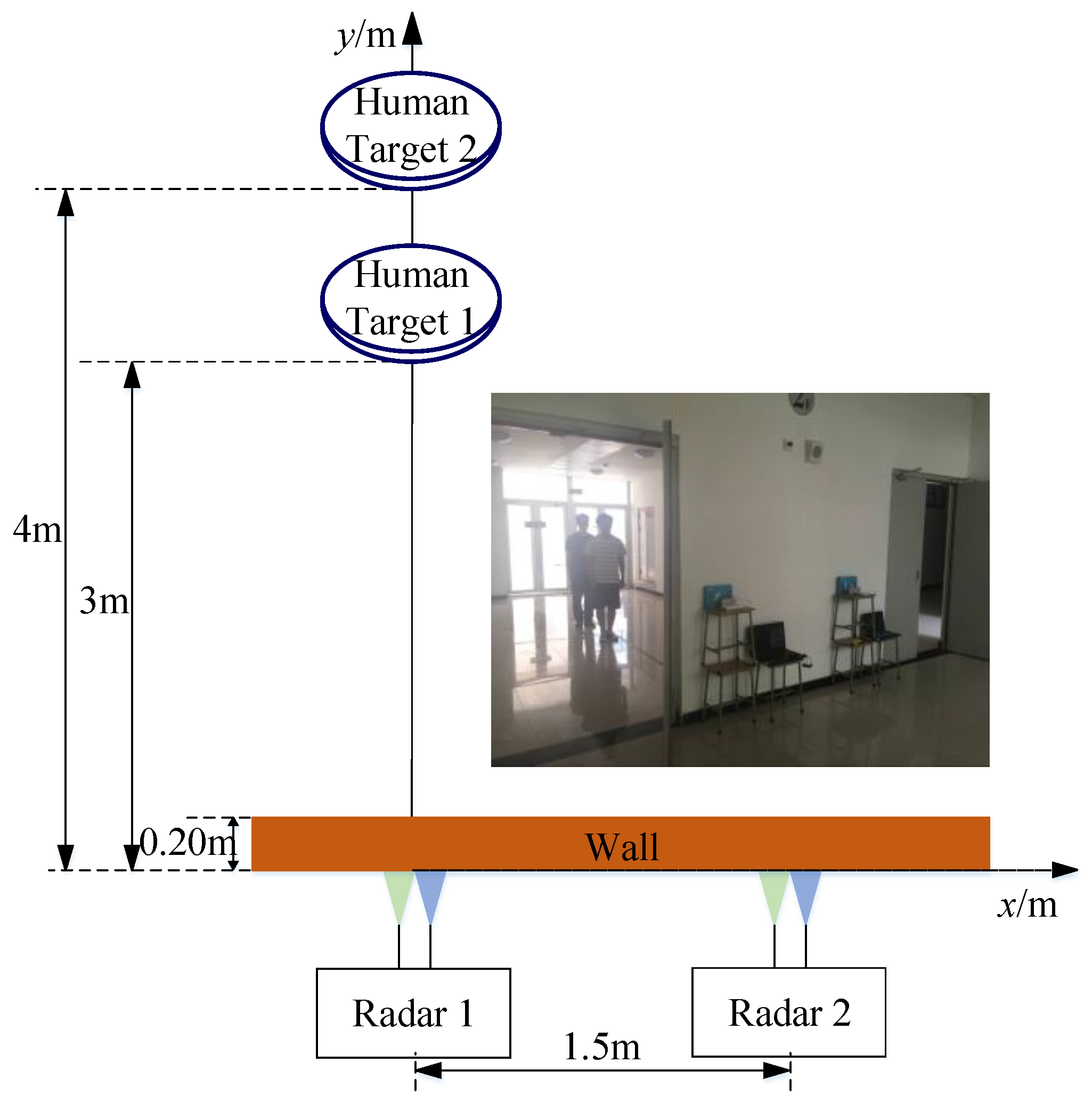
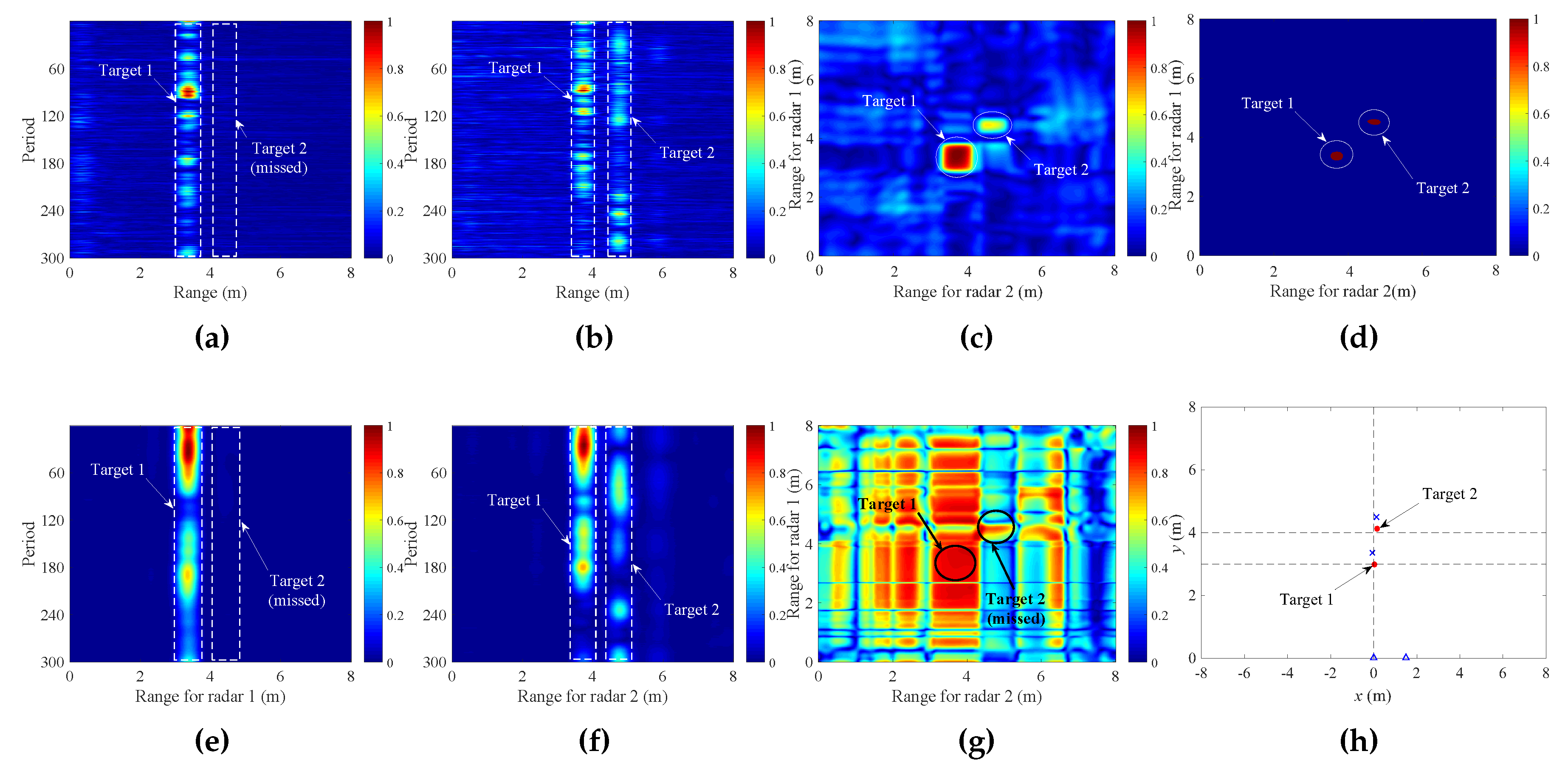
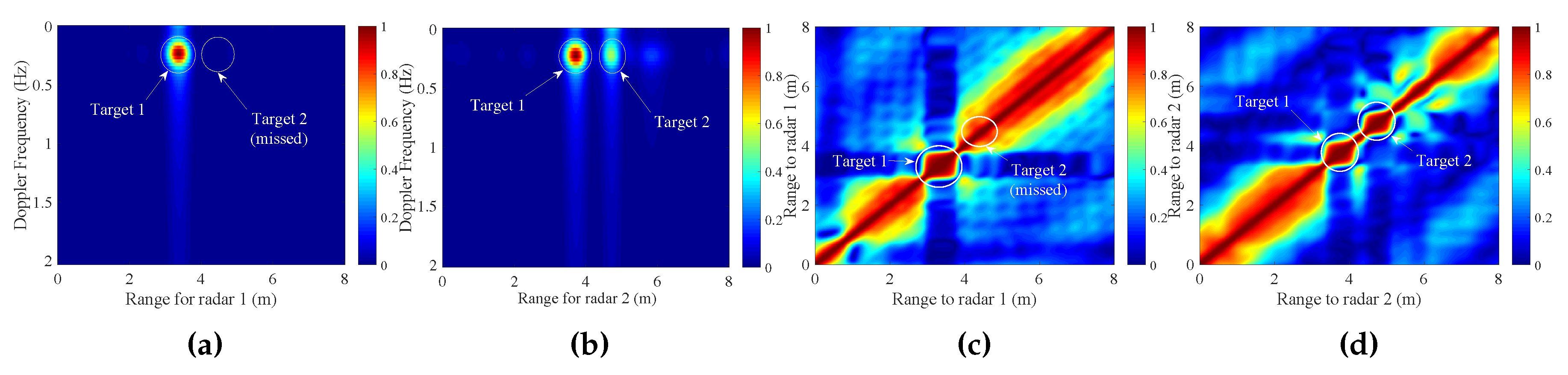
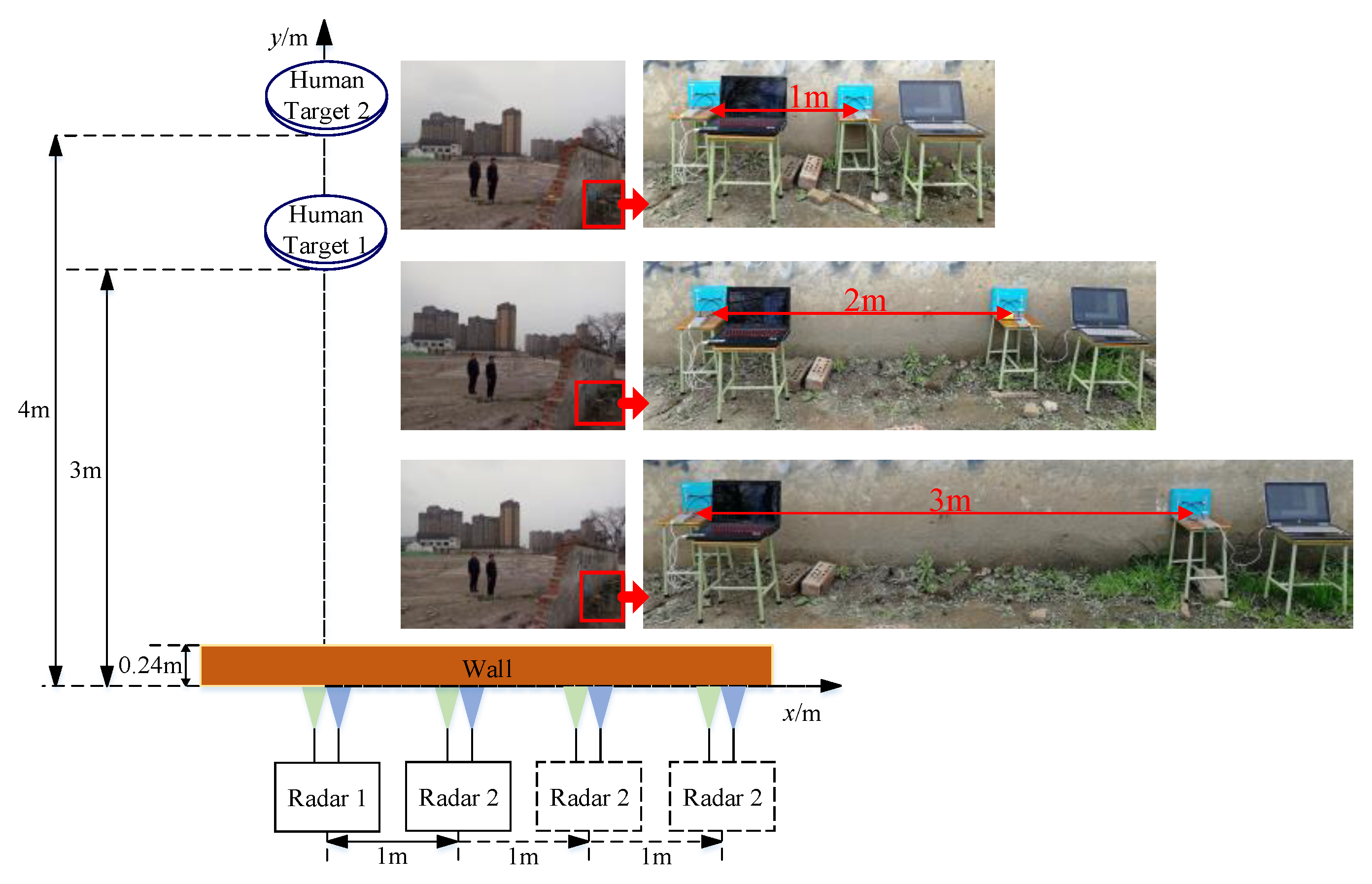
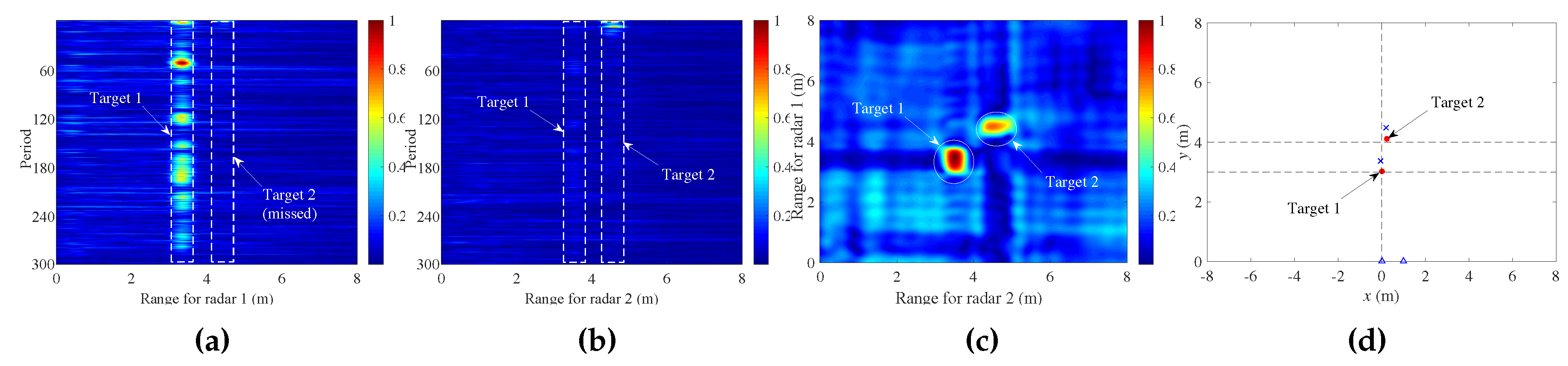
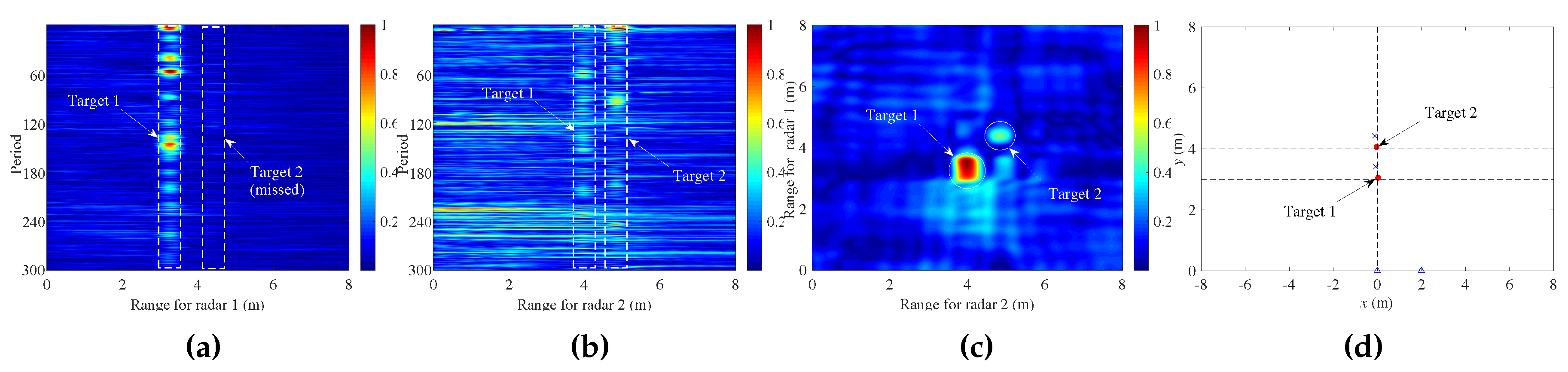
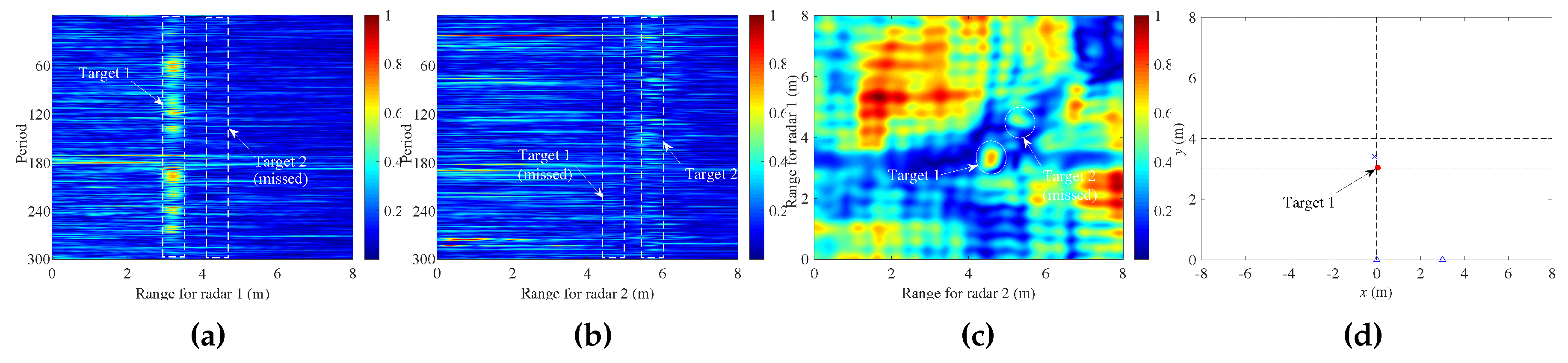
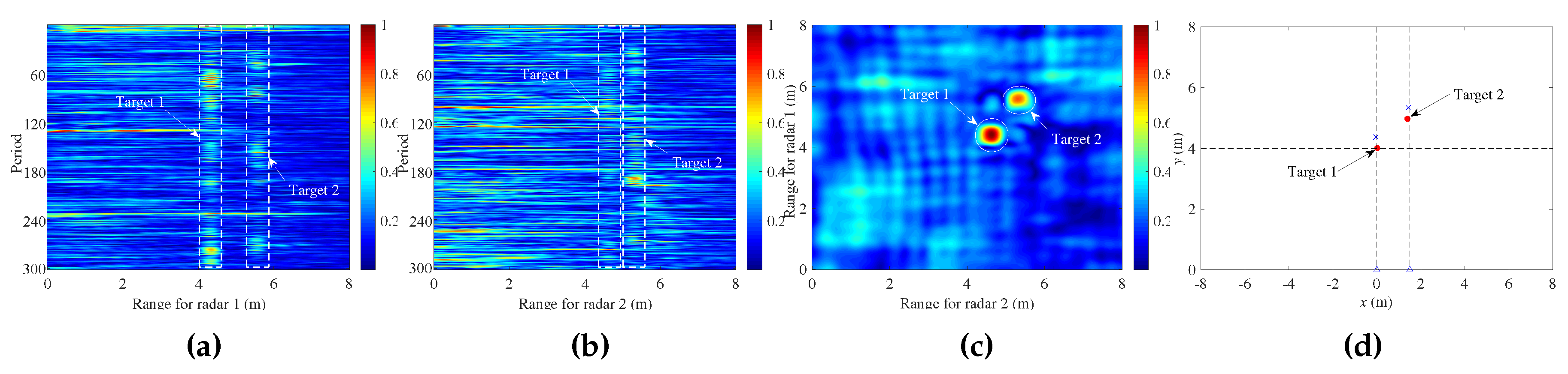
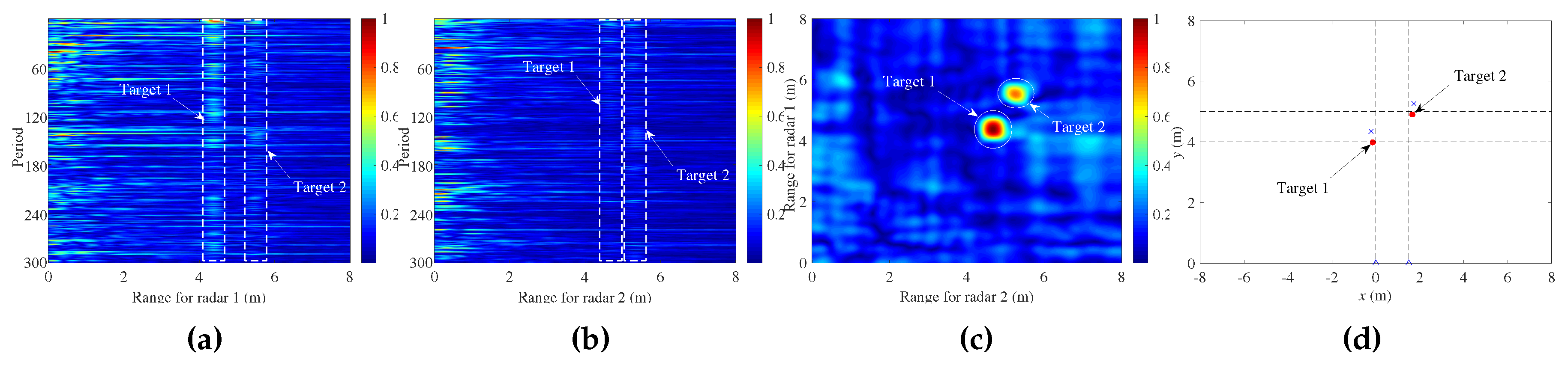
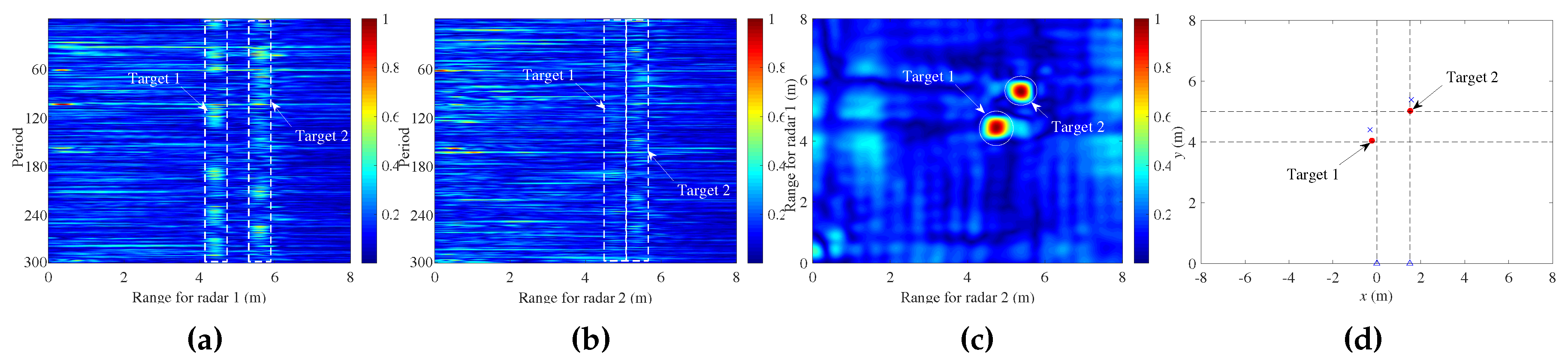
4.2. Experiments with Different Target Positions

The first group of experiments was performed to reveal the effect on the proposed algorithm of different target positions. In these experiments, the wall is a solid brick wall with the measured thickness of 0.2 m and relative permittivity of about 9. As shown in Figure 4, two SFCW radars were placed against the wall with an interval distance of 1.5 m. For the sake of distinction, the experiments are named Experiment 1.1 and Experiment 1.2.

In Experiment 1.1, two human targets with normal respiration were standing at (0 m, 4 m), and (1.5 m, 5 m), based on the given coordinate system, as shown in Figure 5, where Radars 1 and 2 were separately located at the origin of (0 m, 0 m) and (1.5 m, 0 m). Target 1 at (0 m, 4 m) weighs about 75 kg and is about 1.75 m tall. Target 2 at (1.5 m, 5 m) weighs about 70 kg and is about 1.7 m tall. By manually operating the displaying and controlling host computer, the two radars collected $N=300$ periods of SFCW echoes. After IFFT processing with a point number of $M=4096$ and two-pulse cancellation for each period, two fast–slow time range profile planes of the two radars were provided (Figure 6a,b). For ease of observation, the range display was limited from 0 to 8 m. It was obvious that, in the planes of Radar 1, the respiration signal of Target 2 was much lower than that of Target 1 because of the longer propagation range and oblique detection angle of the view while, for Radar 2, the respiration signals of the two targets with approximate propagation ranges and viewing angles had almost identical intensity. Through cross-correlation calculation between the two range profile planes, the correlation coefficient matrix was calculated, as shown in Figure 6c, where two targets clearly emerged. According to the feature of Gaussian distribution [25], it is easy to say that the noise in Figure 6c is non-Gaussian distribution, which means that CFAR detection was unable to provide constant false probability for all matrix elements. Fortunately, two targets were still successfully extracted, as shown in Figure 6d, by pseudo-CFAR detection with $L_c=32$ elements of the sliding window, $L_g=16$ elements of the protection window, and $P_{fa}=0.01$, which verified the feasibility of identifying targets by using a CFAR detector, in this case of non-Gaussian noise background. Each extracted target was composed of multiple conterminous elements with a value of 1, whose centroid element was selected to generate two desired target ranges for two radars by using corresponding row and column coordinates. By placing the extracted target ranges into Equation (15), the estimated target locations were obtained, as shown in Figure 6h with two blue crosses. Because of wall-penetration effect, the estimated target locations were obviously displaced from real target locations. After compensation for wall penetration as in Equation (16), estimations of the target locations were corrected to the vicinities of real locations, marked with two red dots. The coordinates of estimated position of Target 1 and Target 2 are ($-0.09$ m, 4.11 m) and (1.65 m, 5.06 m), respectively.

Mean localization error (MLE) was used to quantitatively evaluate localization accuracy:

$$MLE=\frac{1}{\beta }\sum _{\lambda =1}^{\beta }\sqrt{{\left(x_{\lambda }-{\widehat{x}}_{\lambda }\right)}^2+{\left(y_{\lambda }-{\widehat{y}}_{\lambda }\right)}^2},$$

(17)

where $\beta$ is the total number of targets, x and y are the coordinates of the actual target positions, $\widehat{x}$ and $\widehat{y}$ are the coordinates of the estimated target positions, and $\lambda$ is the target number. The MLE of Experiment 1.1 was about 0.15 m.

Moreover, Figure 6e,f provide the range profile planes of the two radars after an average cancellation of 300 periods. Compared with Figure 6a,b from two-pulse cancellation, the average cancellation had better performance in preserving target signals (with higher SNR), while most associated side lobes were retained as well. Through cross-correlation, the retained side lobes were transformed into widespread ghost interferences, as shown in Figure 6g, hindering the detection of desired main-lobe correlations. Therefore, although the main lobe of the target signal was partly reduced, two-pulse cancellation was a preferred choice for suppressing stationary clutter in the proposed algorithm due to the residual side lobes disappearing in the noise background.

Furthermore, the FFT-based energy accumulation method in [21] and the single-radar correlation based method in [22] were performed to compare the proposed algorithm. Specifically, the FFT accumulation along slow-time was performed on each range profile plane in Figure 6a,b. The generated RD planes are provided in Figure 7a,b where the target ranges and respiration rates could be extracted together. In accordance with Figure 6a, Figure 7a shows that the accumulated respiration signal of Target 2 was much weaker than that of Target 1. In other words, the energy accumulation of FFT inherited the intensity difference of two targets, which made it difficult to identify the weaker target. On the contrary, the two targets were endowed with similar intensities through the proposed cross-correlation operation. Therefore, the aforementioned comparison proved the effectiveness of reducing the intensity difference of multiple targets by cross-correlation of dual-station radars. Besides, through cross-correlation, two ranges of each target associated with two radars were isolated without the additional pairing operation that was necessary for the extracted four target ranges from RD planes in Figure 7a,b.

According to the single-radar correlation-based method in [22], the correlation operation was performed on each range column with regard to each radar plane in Figure 6e,f. As shown in Figure 7c,d, the single-radar correlation results were blurred by widespread ghost interferences derived from the retained side lobes in the average cancellation. Therefore, based on Figure 6g and Figure 7c,d, it is concluded that the average cancellation was unable to support the proposed dual-radar cross-correlation algorithm and the existent single-radar correlation method because of the side lobes of SFCW pulse compression. For simplification, the following dual-radar cross-correlation results and single-radar correlation results were entirely based on the range profile planes from the two-pulse cancellation. Specially, Figure 7e,f reveals the single-radar correlation results corresponding to the range profile planes in Figure 6a,b from two-pulse cancellation, where ghost interferences were significantly reduced in contrast to Figure 7c,d. However, it was also difficult based on the single-radar correlation method to identify weak Target 2 from the results in Figure 7e. It is noticed that, in Figure 7c–f, there exist line-like interferences around the diagonal that adversely affected the target detection. The line-like interference is an inherent defect in the single-radar correlation algorithm [22] because the correlation coefficient between the data vector in each range unit and itself is always 1.

To evaluate cross-correlation performance under extreme conditions, Experiment 1.2 was implemented as shown in Figure 8 where two human targets stood in a line along with y-axis. In this case, with regard to Radar 1, the far Target 2 at (0 m, 4 m) fell into the shadow of the near Target 1 at (0 m, 3 m). The target at (0 m, 3 m) weighs about 70 kg and is about 1.7 m tall. The target at (0 m, 4 m) weighs about 75 kg and is about 1.75 m tall. Therefore, from the range profile plane in Figure 9a and the RD plane in Figure 10a of Radar 1, the respiration signal of Target 2 almost disappeared. It was verified that the existing method based on energy accumulation suffered from the problem of missed detection of weak target. Meanwhile, as given in Figure 9b,d for Radar 2, the respiration signals of two targets were captured from another angle of view without a shadow effect, while Target 2 was weaker than Target 1 due to the longer propagation range. Fortunately, by utilizing the proposed algorithm based on dual-station cross-correlation, the weak Target 2 also appeared clearly (Figure 9c) and was thus detected successfully (Figure 9d). Furthermore, two pairs of ranges of two targets were obtained to generate the estimation target locations with wall compensation, as shown in Figure 9h. The coordinates of estimated positions of Target 1 and Target 2 were (0.06 m, 2.95 m) and (0.05 m, 4.12 m), respectively. The MLE was about 0.1 m. It was demonstrated that the cross-correlation operation was able to support robust detection and localization of multiple different intensities of stationary human targets even in the case of a shadowing effect, by exploring the correlation characteristic of each target between two radars.

Moreover, although two range profile planes of average cancellation had a higher SNR, as shown in Figure 9e,f, the corresponding cross-correlation result in Figure 9g was seriously blurred by widespread ghost interferences from the retained side lobes. It was further demonstrated that the average cancellation was unavailable to the proposed cross-correlation algorithm with dual SFCW radars. Figure 10c,d shows the single-radar correlation results, as in [22]. Obviously, the shadowed weak Target 2 for Radar 1 was missed, as shown in Figure 10c. By comparing with Figure 9c, the superiority of the proposed algorithm in weak target detection was validated, guaranteed by two-view observation of dual-station radars because the shadowed weak target in one radar view can be observed effectively in another radar view.

4.3. Experiments with Different Radar Locations

For a comprehensive verification of the proposed algorithm, the following three groups of experiments were accomplished in the other scenes to study the effects of radar location, human-target orientation, and human-target posture. The wall in these three groups of experiments was a solid brick wall with a measured thickness of 0.24 m and relative permittivity of about 8.5. The height of the radar antennas from the ground was 0.54 m. The body type of one human target was about 75 kg weight and 1.7 m height, and the other human target was about 65 kg weight and 1.7 m height.

In this subsection, three experiment results are provided to observe the effect of different radar locations. Specifically, under the fixed origin location of Radar 1, Radar 2 was moved away from Radar 1 in a straight line to separately form three interval distances of two radars, namely 1 m, 2 m and 3 m, corresponding to three experiments, as shown in Figure 11. In these three experiments, the two human targets stood at coordinates of (0 m, 3 m) and (0 m, 4 m) as in Experiment 1.2. For simplification, the three experiments with the radar intervals of 1 m, 2 m and 3 m are denoted by Experiments 2.1, 2.2 and 2.3, respectively. The coordinates of estimated target positions and MLE of the experiments above are shown in

Table 3. Localization results and MLE of Experiment 2.

	Experiment 2.1	Experiment 2.2	Experiment 2.3
Extracted coordinates of Target 1	(0.02 m, 3.02 m)	(0.04 m, 3.05 m)	(0.04 m, 3.04 m)
Extracted coordinates of Target 2	(0.22 m, 4.11 m)	(−0.03 m, 4.06 m)	Missed detection
MLE	0.14 m	0.07 m	N/A

.

The experimental results including range profiles of two radars, cross-correlation images, and localization result, are provided in Figure 12, Figure 13 and Figure 14 for Experiments 2.1–2.3, respectively. By comparison, it can be seen that, with the increase of radar interval, the two targets, especially Target 2, gradually disappeared in the clutter background. That is because, in the case of a larger radar interval, the greater ranges and the bigger observation angles between Radar 2 and the two targets reduced respiration-signal intensities. Especially under the joint action of target occlusion, Target 2 was out of the effective detection and localization range of the proposed cross-correlation algorithm.

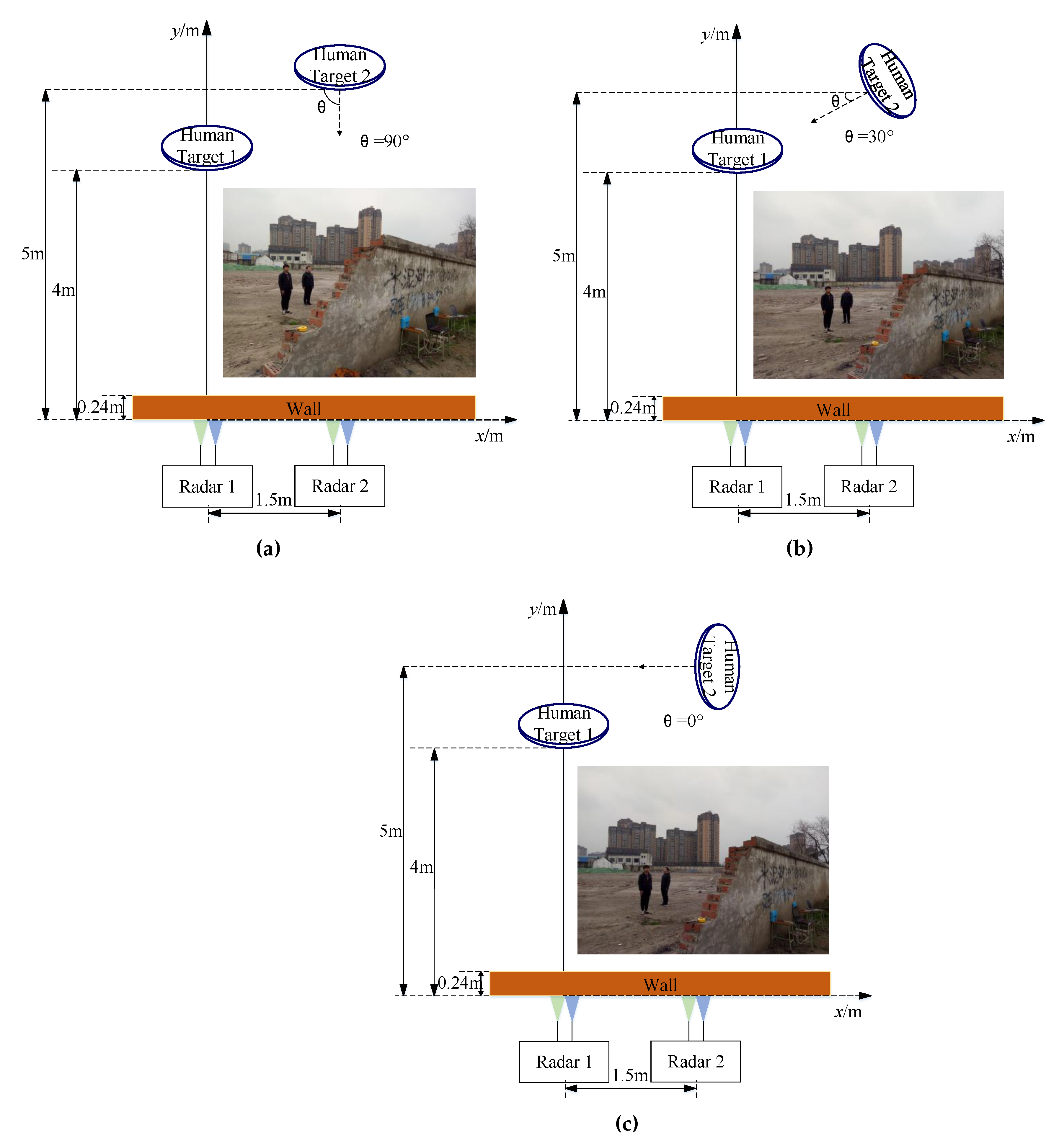
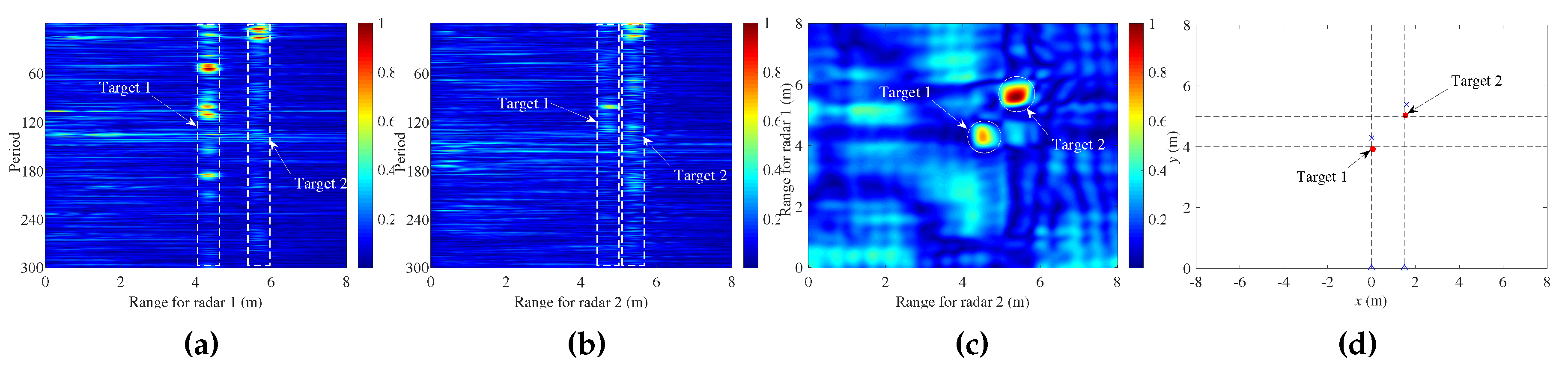
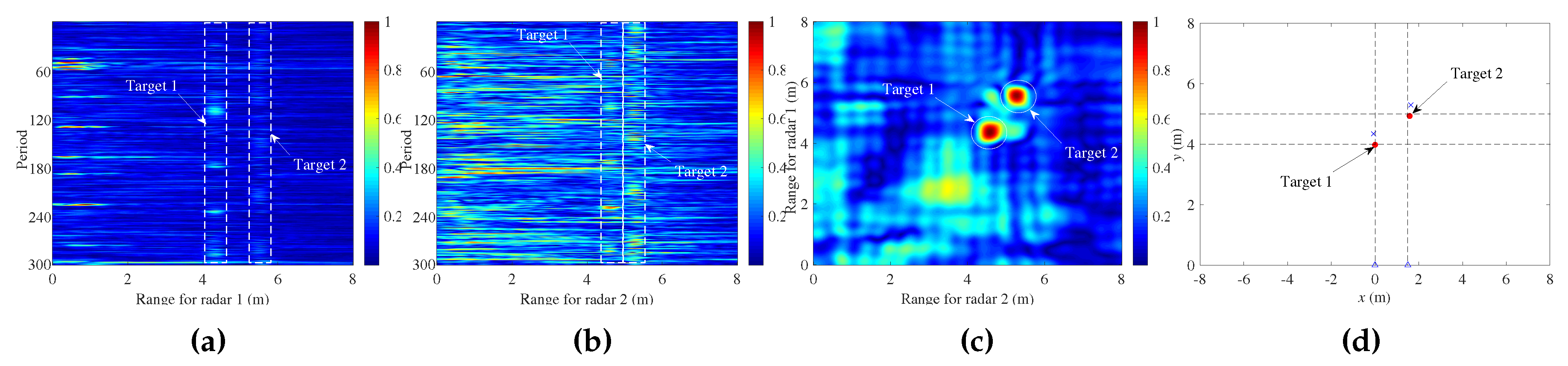
4.4. Experiments with Different Target Orientations

In this subsection, the influence of target orientation was considered by carrying out three experiments with different orientations of human Target 2, as shown in Figure 15. These two radars were located at (0 m, 0 m) and (1.5 m, 0 m) as in Experiments 1.1 and 1.2, and the two human targets stood at (0 m, 4 m) and (1.5 m, 5 m), respectively. In these three experiments, Target 1 maintained a fixed orientation that was always facing Radar 1, while Target 2 was endowed with three different orientations, namely, three orientation angles of $0^{\circ }$, ${30}^{\circ }$, and ${90}^{\circ }$ between target orientation and the baseline of the two radars. For convenience, these three experiments in Figure 15a–c are labeled Experiments 3.1, 3.2, and 3.3, respectively. The coordinates of estimated target positions and MLE of the experiments above are shown in

Table 4. Localization results and MLE of Experiment 3.

	Experiment 3.1	Experiment 3.2	Experiment 3.3
Extracted coordinates of Target 1	(0.06 m, 3.92 m)	(0 m, 3.98 m)	(−0.11 m, 3.93 m)
Extracted coordinates of Target 2	(1.54 m, 5.03 m)	(1.58 m, 4.94 m)	(1.43 m, 5.04 m)
MLE	0.08 m	0.06 m	0.11 m

.

As shown in Figure 16a,b, Figure 17a,b, and Figure 18a,b, the respiration signals of Target 2 in the range profile planes of the two radars fell into a decline along with the decrease of orientation angle from ${90}^{\circ }$ to $0^{\circ }$. In the case of an orientation angle of $0^{\circ }$, it was almost impossible to identify the respiration signals in these two range profile planes. That is because the major fluctuations of the human abdomen, caused by respiration, gradually deviated from the observation view of the two radars, while the affiliated minor fluctuations of the scapula part gradually turned toward the radar view. Fortunately, through the presented cross-correlation process, these two targets were clearly highlighted in the cross-correlation images, as shown in Figure 16c, Figure 17c, and Figure 18c. Therefore, through CFAR detection, the range of two targets could be successfully extracted to calculate estimations of target locations, as shown in Figure 16d, Figure 17d, and Figure 18d. Based on the above discussion, it was demonstrated that the proposed cross-correlation algorithm has the favorable ability to adapt different orientations of human targets.

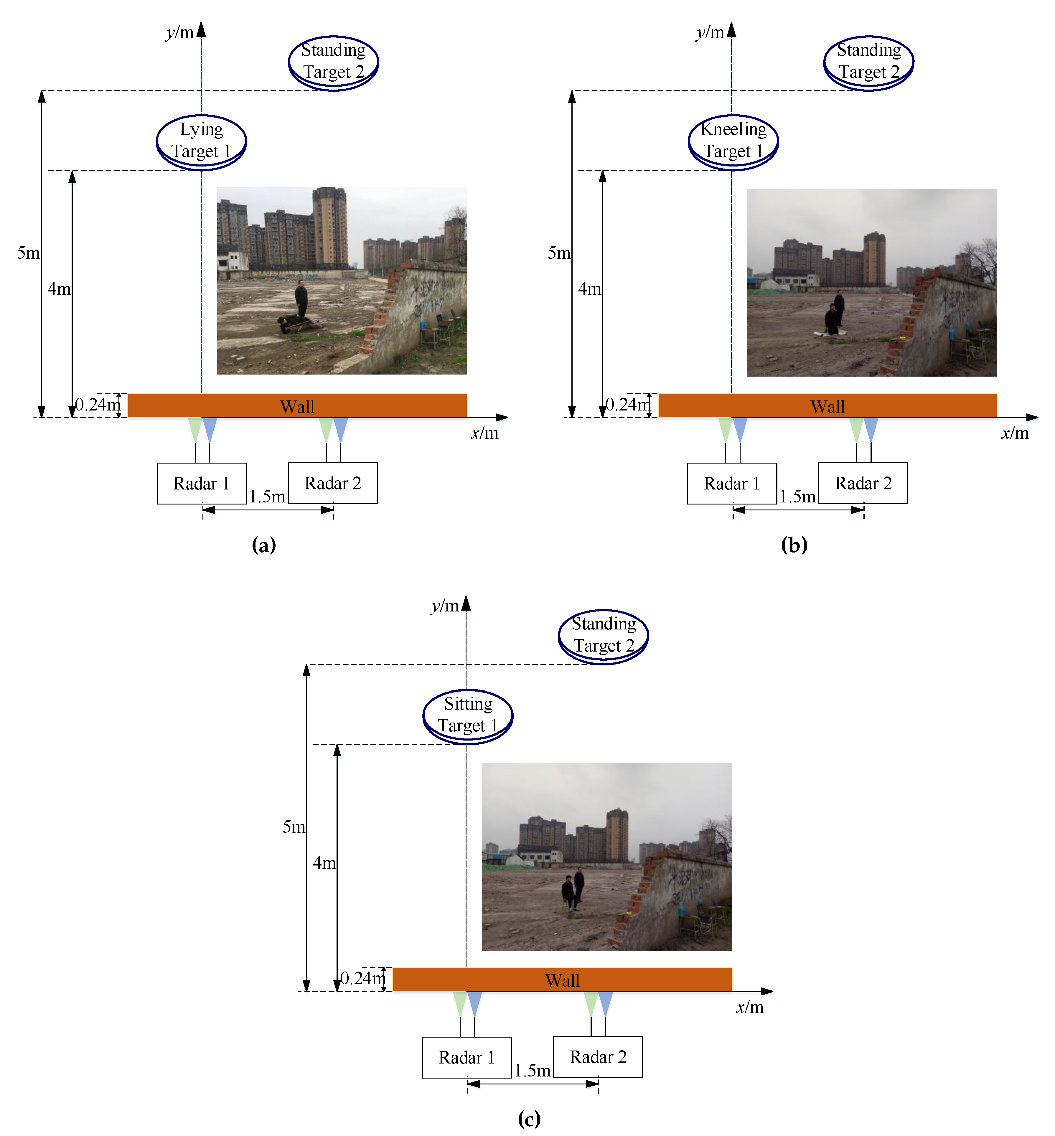
4.5. Experiments with Different Target Postures

To evaluate the algorithm performance for different human target postures, three experimental results with three additional postures including lying, kneeling and sitting are provided in this subsection. As shown in Figure 19, for these three experiments, Radar 1 and Radar 2 were always located at (0 m, 0 m) and (1.5 m, 0 m), and the human Target 1 and Target 2 were invariably positioned at (0 m, 4 m) and (1.5 m, 5 m). Moreover, in each experiment, Target 2 maintained the posture of standing as a reference, while Target 1 was assigned with different postures. For simplification, these three experiments in Figure 19a–c are represented separately by Experiments 4.1, 4.2 and 4.3 with regard to lying, kneeling and sitting of Target 2, respectively. The coordinates of estimated target positions and MLE of the experiments above are shown in

Table 5. Localization results and MLE of Experiment 4.

	Experiment 4.1	Experiment 4.2	Experiment 4.3
Extracted coordinates of Target 1	(0.02 m, 4.01 m)	(−0.14 m, 3.99 m)	(−0.06 m, 4.02 m)
Extracted coordinates of Target 2	(1.39 m, 4.97 m)	(1.66 m, 4.91 m)	(1.69 m, 4.94 m)
MLE	0.07 m	0.16 m	0.13 m

.

Figure 20, Figure 21 and Figure 22 show that, although these two targets with postures of standing, lying, kneeling, and sitting ambiguously appeared in the range profiles, the cross-correlation process could still clear the targets in the correlation images, ensuring the feasibility of the subsequent detection and localization. Therefore, the proposed cross-correlation algorithm could be applied to detect and localize multiple different postures of human targets.

For all the above experiments, data processing was implemented on a laptop with Windows using MATLAB software. The laptop has an Intel Core i5 CPU with a frequency of 2.5 GHz and a memory of 8 GB. For the interesting range interval of 8 m, the average time consumption of the proposed algorithm was about 14.67 s.

5. Conclusions

A cross-correlation algorithm of dual-station SFCW radars is designed to implement detection and localization of multiple stationary human targets. The application of SFCW signals makes it feasible to implement simultaneous dual-view observation without mutual interference by deploying two single-channel radars at different stations. Based on the correlation characteristics of respiration signals of each target between the two radars, the cross-correlation coefficient matrix of two-radar target echoes is first calculated. Then, a two-dimension CFAR detector is employed to extract the range of multiple targets from the cross-correlation coefficient matrix. Finally, the extracted target ranges are transformed to the estimations of target locations by utilizing a triangulation method.

Based on multiple groups of experiment results in two different scenes and multiple different setups, we conclude the following three points about the presented cross-correlation algorithm. First, compared with the existent energy-accumulation algorithm and single-radar correlation algorithm, the missed detection of weak targets can be efficiently prevented, even in the case of target occlusion for one of the two radars. Second, necessary additional range pairing in the existent single-radar processing algorithm is avoided because two ranges of each target for the two radars are synchronously connected in the cross-correlation process. Finally, the cross-correlation algorithm has favorable adaptability for different radar locations, human-target orientations, and postures, except for the condition of large radar intervals with a large observation angle. As a conclusion, the proposed dual-station cross-correlation algorithm provides an effective integrated approach for the detection and localization of multiple stationary human targets.

References

1. Mazhar, F.; Khan, M.G.; Sällberg, B. Precise Indoor Positioning Using UWB: A Review of Methods, Algorithms and Implementations. Wirel. Pers. Commun. 2017, 97, 4467–4491. [Google Scholar] [CrossRef]
2. Hu, H.B.; Lin, G.H.; He, H.; Zhang, Y.M. A Review of Research of Life Detecting Radar. Appl. Mech. Mater. 2014, 519–520, 1139–1143. [Google Scholar] [CrossRef]
3. Shi, L.; Jiang, M.; Huang, L. Human status recognition method for the life detection radarbased on the harmonic model. J. Xidian Univ. 2005, 32, 179–183. [Google Scholar] [CrossRef]
4. Lubecke, V.M.; Boric-Lubecke, O.; Host-Madsen, A.; Fathy, A.E. Through-the-Wall Radar Life Detection and Monitoring. In Proceedings of the 2007 IEEE/MTT-S International Microwave Symposium, Honolulu, HI, USA, 3–8 June 2007; pp. 769–772. [Google Scholar] [CrossRef]
5. Lu, G.H.; Wang, J.Q.; Yang, G.S. Current state of the technology of bioradar. Foreign Med. Biomed. Eng. Fasc. 2004. [Google Scholar]
6. Liu, J.; Jia, Y.; Kong, L.; Yang, X.; Liu, Q.H. MIMO through-wall radar 3-D imaging of a human body in different postures. J. Electromagn. Waves Appl. 2016, 30, 849–859. [Google Scholar] [CrossRef]
7. Jia, Y.; Zhong, X.; Liu, J.; Guo, Y. Single-Side Two-Location Spotlight Imaging for Building Based on MIMO Through-Wall-Radar. Sensors 2016, 16, 1441. [Google Scholar] [CrossRef] [PubMed]
8. Liu, J.; Jia, Y.; Kong, L.; Yang, X.; Liu, Q.H. Sign-Coherence-Factor-Based Suppression for Grating Lobes in Through-Wall Radar Imaging. IEEE Geosci. Remote Sens. Lett. 2016, 13, 1681–1685. [Google Scholar] [CrossRef]
9. Cippitelli, E.; Fioranelli, F.; Gambi, E.; Spinsante, S. Radar and RGB-Depth Sensors for Fall Detection: A Review. IEEE Sens. J. 2017, 17, 3585–3604. [Google Scholar] [CrossRef] [Green Version]
10. Zhang, J.; Jin, T.; He, Y.M.; Zhou, Z. A Centralized Processing Framework for Foliage Penetration Human Tracking in Multistatic Radar. Radioengineering 2016, 25, 98–105. [Google Scholar] [CrossRef]
11. Caro, C.G.; Bloice, J.A. Contactless apnoea detector based on radar. Lancet 1971, 2, 959–961. [Google Scholar] [CrossRef]
12. Tateishi, N.; Mase, A.; Bruskin, L.; Kogi, Y.; Ito, N.; Shirakata, T.; Yoshida, S. Microwave Measurement of Heart Beat and Analysis Using Wavelet Transform. In Proceedings of the 2007 Asia-Pacific Microwave Conference, Bangkok, Thailand, 11–14 December 2007; pp. 2151–2153. [Google Scholar] [CrossRef]
13. Chen, K.M.; Huang, Y.; Zhang, J.; Norman, A. Microwave life-detection systems for searching human subjects under earthquake rubble or behind barrier. IEEE Trans. Biomed. Eng. 2000, 47, 105–114. [Google Scholar] [CrossRef] [PubMed]
14. Yarovoy, A.G.; Ligthart, L.P.; Matuzas, J.; Levitas, B. UWB radar for human being detection. IEEE Aerosp. Electron. Syst. Mag. 2006, 21, 10–14. [Google Scholar] [CrossRef] [Green Version]
15. Anitori, L.; de Jong, A.; Nennie, F. FMCW radar for life-sign detection. In Proceedings of the 2009 IEEE Radar Conference, Pasadena, CA, USA, 4–8 May 2009; pp. 1–6. [Google Scholar] [CrossRef]
16. Guo, S.; Cui, G.; Kong, L.; Yang, X. An Imaging Dictionary Based Multipath Suppression Algorithm for Through-Wall Radar Imaging. IEEE Trans. Aerosp. Electron. Syst. 2018, 54, 269–283. [Google Scholar] [CrossRef]
17. Guo, S.; Cui, G.; Wang, M.; Kong, L.; Yang, X. Similarity-based multipath suppression algorithm for through-wall imaging radar. IET Radar Sonar Navig. 2017, 11, 1041–1050. [Google Scholar] [CrossRef]
18. Qiu, L.; Jin, T.; Lu, B.; Zhou, Z. An Isophase-Based Life Signal Extraction in Through-the-Wall Radar. IEEE Geosci. Remote Sens. Lett. 2017, 14, 193–197. [Google Scholar] [CrossRef]
19. Phelan, B.R.; Ranney, K.I.; Gallagher, K.A.; Clark, J.T.; Sherbondy, K.D.; Narayanan, R.M. Design of Ultrawideband Stepped-Frequency Radar for Imaging of Obscured Targets. IEEE Sens. J. 2017, 17, 4435–4446. [Google Scholar] [CrossRef]
20. Yılmaz, B.; Özdemir, C. A detection and localization algorithm for moving targets behind walls based on one transmitter-two receiver configuration. Microw. Opt. Technol. Lett. 2017, 59, 1252–1259. [Google Scholar] [CrossRef]
21. Jia, Y.; Kong, L.; Yang, X.; Wang, K. Through-wall-radar localization for stationary human based on life-sign detection. In Proceedings of the 2013 IEEE Radar Conference (RadarCon13), Ottawa, ON, Canada, 29 April–3 May 2013; pp. 1–4. [Google Scholar] [CrossRef]
22. Zhang, Y.; Chen, F.; Xue, H.; Li, Z.; An, Q.; Wang, J. Detection and Identification of Multiple Stationary Human Targets Via Bio-Radar Based on the Cross-Correlation Method. Sensors 2016, 16, 1793. [Google Scholar] [CrossRef] [PubMed]
23. Yan, S.; Kong, L.; Yang, X.; Zhou, Y. Life detection based on cross-correlation analysis. In Proceedings of the 2011 IEEE CIE International Conference on Radar, Chengdu, China, 24–27 October 2011; Volume 2, pp. 1346–1348. [Google Scholar] [CrossRef]
24. Conte, E.; De Maio, A.; Ricci, G. Recursive estimation of the covariance matrix of a compound-Gaussian process and its application to adaptive CFAR detection. IEEE Trans. Signal Process. 2002, 50, 1908–1915. [Google Scholar] [CrossRef]
25. Xu, S.W.; Shui, P.L. Range-spread target detection in white Gaussian noise via two-dimensional non-linear shrinkage map and geometric average integration. IET Radar Sonar Navig. 2012, 6, 90–98. [Google Scholar] [CrossRef]
Figure 1. Dual-station SFCW radars.
Remotesensing 11 01428 g001
Figure 2. Detection and localization flowchart based on dual-station cross-correlation.
Remotesensing 11 01428 g002
Figure 3. Block diagram of the single-channel SFCW radar.
Remotesensing 11 01428 g003
Figure 4. Deployment of dual-station radars.
Remotesensing 11 01428 g004
Figure 5. Photograph and geometry of Experiment 1.1.
Remotesensing 11 01428 g005
Figure 6. Results of Experiment 1.1: (a) range profile plane of two-pulse cancellation for Radar 1; (b) range profile plane of two-pulse cancellation for Radar 2; (c) cross-correlation result between (a,b); (d) CFAR detection result; (e) range profile plane of average cancellation for Radar 1; (f) range profile plane of average cancellation for Radar 2; (g) cross-correlation result between (e,f); and (h) localization result.
Remotesensing 11 01428 g006
Figure 7. Comparison results of Experiment 1.1: (a) RD plane of Figure 6e; (b) RD plane of Figure 6f; (c) single-radar correlation result of Figure 6e; (d) single-radar correlation result of Figure 6f; (e) single-radar correlation result of Figure 6a; and (f) single-radar correlation result of Figure 6b.
Remotesensing 11 01428 g007
Figure 8. Photograph and geometry of Experiment 1.2.
Remotesensing 11 01428 g008
Figure 9. Results of Experiment 1.2: (a) range profile plane for Radar 1; (b) range profile plane for Radar 2; (c) cross-correlation result between (a,b); (d) CFAR detection result; (e) range profile plane of average cancellation for Radar 1; (f) range profile plane of average cancellation for Radar 2; (g) cross-correlation result between (e,f); and (h) localization result.
Remotesensing 11 01428 g009
Figure 10. Comparison results of Experiment 1.2: (a) RD plane of Figure 9e; (b) RD plane of Figure 9f; (c) single-radar correlation result of Figure 9e; and (d) single-radar correlation result of Figure 9f.
Remotesensing 11 01428 g010
Figure 11. Photographs and geometries of Experiment 2.
Remotesensing 11 01428 g011
Figure 12. Results of Experiment 2.1 with 1 m interval between two radars: (a) range profile plane for Radar 1; (b) range profile plane for Radar 2; (c) cross-correlation image; and (d) localization result.
Remotesensing 11 01428 g012
Figure 13. Results of Experiment 2.2 with 2 m interval between two radars: (a) range profile plane for Radar 1; (b) range profile plane for Radar 2; (c) cross-correlation image; and (d) localization result.
Remotesensing 11 01428 g013
Figure 14. Results of Experiment 2.3 with 3 m interval between two radars: (a) range profile plane for Radar 1; (b) range profile plane for Radar 2; (c) cross-correlation image; and (d) localization result.
Remotesensing 11 01428 g014
Figure 15. Photographs and geometries of Experiment 3: (a) Experiment 3.1 with orientation angle of 90 for Target 2; (b) Experiment 3.2 with orientation angle of 30 for Target 2; and (c) Experiment 3.3 with orientation angle of 0 for Target 2.
Remotesensing 11 01428 g015
Figure 16. Results of Experiment 3.1: (a) range profile plane for Radar 1; (b) range profile plane for Radar 2; (c) cross-correlation image; and (d) localization result.
Remotesensing 11 01428 g016
Figure 17. Results of Experiment 3.2: (a) range profile plane for Radar 1; (b) range profile plane for Radar 2; (c) cross-correlation image; and (d) localization result.
Remotesensing 11 01428 g017
Figure 18. Results of Experiment 3.3: (a) range profile plane for Radar 1; (b) range profile plane for Radar 2; (c) cross-correlation image; and (d) localization result.
Remotesensing 11 01428 g018
Figure 19. Photographs and geometries of Experiment 4: (a) Experiment 4.1 with lying posture for Target 1; (b) Experiment 4.2 with kneeling posture for Target 1; and (c) Experiment 4.3 with sitting posture for Target 1.
Remotesensing 11 01428 g019
Figure 20. Results of Experiment 4.1: (a) range profile plane for Radar 1; (b) range profile plane for Radar 2; (c) cross-correlation image; and (d) localization result.
Remotesensing 11 01428 g020
Figure 21. Results of Experiment 4.2: (a) range profile plane for Radar 1; (b) range profile plane for Radar 2; (c) cross-correlation image; and (d) localization result.
Remotesensing 11 01428 g021
Figure 22. Results of Experiment 4.3: (a) range profile plane for Radar 1; (b) range profile plane for Radar 2; (c) cross-correlation image; and (d) localization result.
Remotesensing 11 01428 g022