Modelling the Wealth Index of Demographic and Health Surveys within Cities Using Very High-Resolution Remotely Sensed Information

 ,
,  , , , and
Abstract
1. Introduction
2. Materials and Methods
2.1. Overview
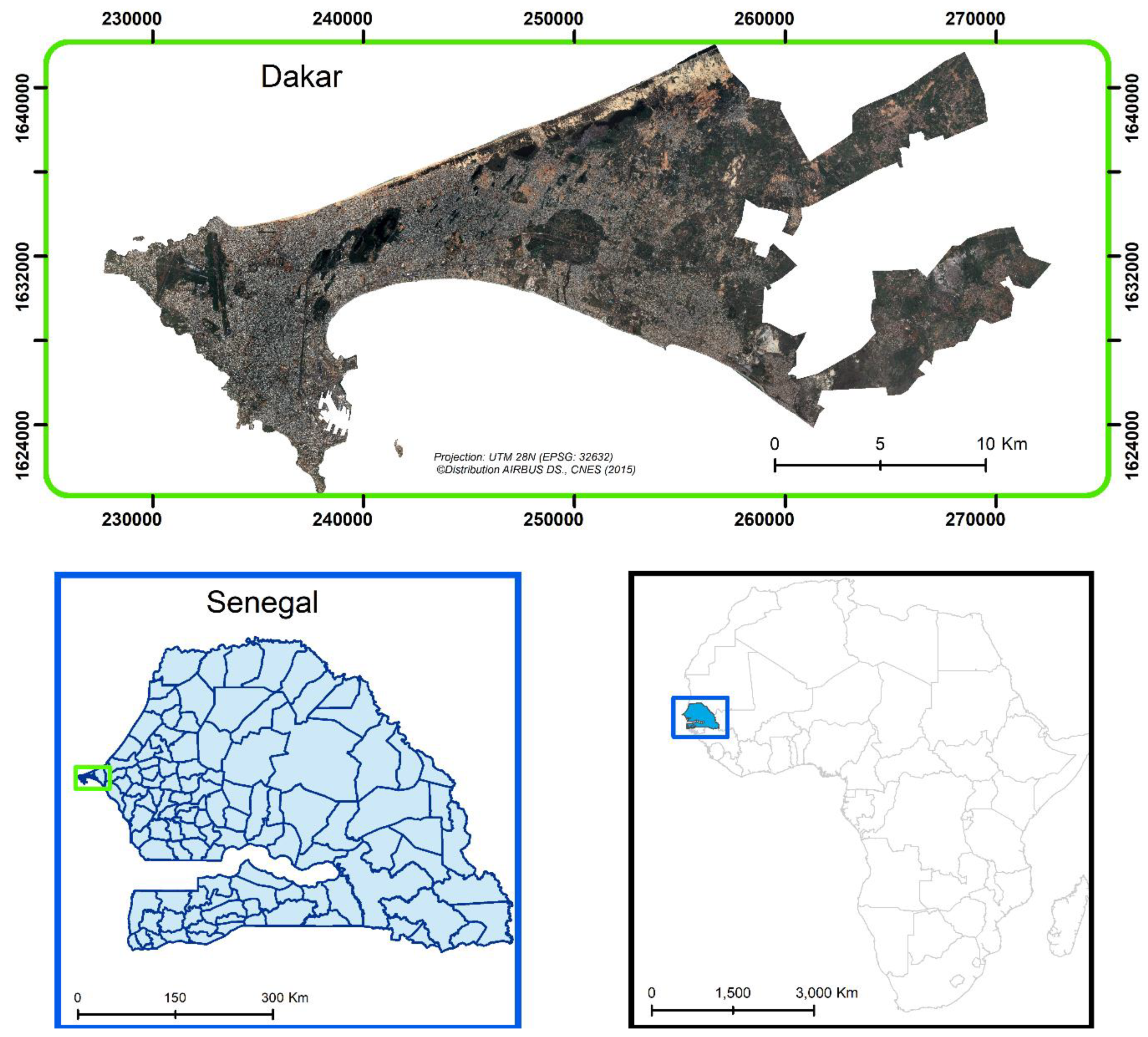
2.2. Study Area
2.3. Demographic and Health Surveys (DHS)
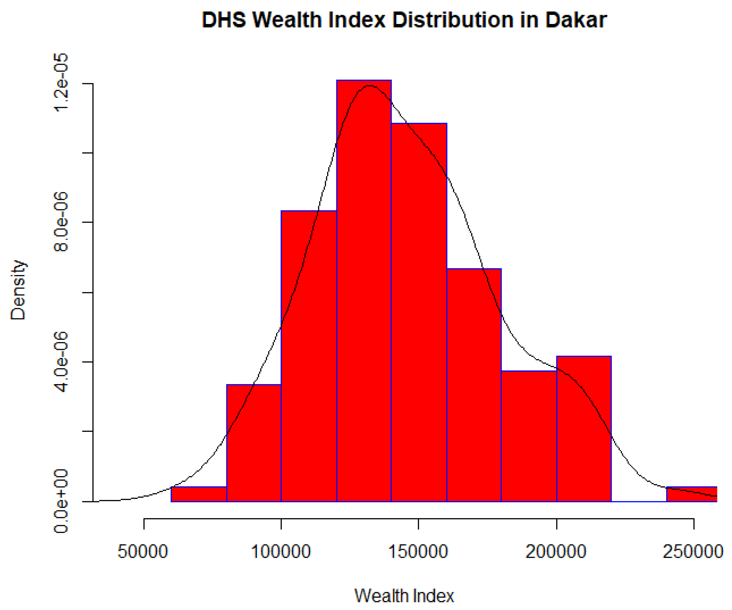
DHS Wealth Index (WI)
2.4. Very High-Resolution (VHR) Satellite Data
2.5. Model Selection and Spatial Optimization Methods
2.6. Validation Scheme
2.6.1. Validation at the DHS Survey Level
2.6.2. Validation at the Census Level
3. Results
3.1. DHS WI Models
3.2. Validation
4. Discussion
5. Conclusions
Author Contributions
Funding
Acknowledgments
Conflicts of Interest
References
- Prashad, V. The Poorer Nations: A Possible History of the Global South; London Verso Trade: London, UK, 2013. [Google Scholar]
- Weiss, T.G. The United Nations and Changing World Politics; Routledge: Abingdon, UK, 2018. [Google Scholar]
- Stoler, J.; Daniels, D.; Weeks, J.R.; Stow, D.A.; Coulter, L.L.; Finch, B.K. Assessing the Utility of Satellite Imagery with Differing Spatial Resolutions for Deriving Proxy Measures of Slum Presence in Accra, Ghana. GISci. Remote Sens. 2012, 49, 31–52. [Google Scholar] [CrossRef] [PubMed]
- Weeks, J.R.; Hill, A.; Stow, D.; Getis, A.; Fugate, D. Can we spot a neighborhood from the air? {Defining} neighborhood structure in {Accra}, {Ghana}. GeoJournal 2007, 69, 9–22. [Google Scholar] [CrossRef] [PubMed]
- Engstrom, R.; Hersh, J.; Newhouse, D. Poverty in HD: What Does High Resolution Satellite Imagery Reveal about Economic Welfare? Available online: Pubdocs.worldbank.org/en/60741466181743796/Poverty-in-HD-draft-v2-75.pdf (accessed on 1 December 2016).
- Bosco, C.; Alegana, V.; Bird, T.; Pezzulo, C.; Bengtsson, L.; Sorichetta, A.; Steele, J.; Hornby, G.; Ruktanonchai, C.; Ruktanonchai, N.; et al. Exploring the high-resolution mapping of gender-disaggregated development indicators. J. R. Soc. Interface 2017, 14, 20160825. [Google Scholar] [CrossRef] [PubMed]
- Stevens, F.R.; Gaughan, A.E.; Linard, C.; Tatem, A.J. Disaggregating census data for population mapping using Random forests with remotely-sensed and ancillary data. PLoS ONE 2015, 10, 1–22. [Google Scholar] [CrossRef] [PubMed]
- Corsi, D.J.; Neuman, M.; Finlay, J.E.; Subramanian, S.V. Demographic and health surveys: A profile. Int. J. Epidemiol. 2012, 41, 1602–1613. [Google Scholar] [CrossRef] [PubMed]
- Gething, P.W.; Tatem, A.J.; Bird, T.; Burgert, C. Creating Spatial Interpolation Surfaces with DHS Data; DHS Program: Rockville, MD, UDA, 2015. [Google Scholar]
- Weeks, J.R.; Getis, A.; Stow, D.A.; Hill, A.G.; Rain, D.; Engstrom, R.; Stoler, J.; Lippitt, C.; Jankowska, M.; Lopez-Carr, A.C.; et al. Connecting the Dots Between Health, Poverty and Place in Accra, Ghana. Ann. Assoc. Am. Geogr. 2012, 102, 932–941. [Google Scholar] [CrossRef]
- Tapiador, F.J.; Avelar, S.; Tavares-corrêa, C.; Zah, R.; Tapiador, F.J.; Avelar, S.; Tavares-corrêa, C. Deriving fine-scale socioeconomic information of urban areas using very high-resolution satellite imagery. Int. J. Remote Sens. 2011, 32, 6437–6456. [Google Scholar] [CrossRef]
- Avelar, S.; Zah, R.; Tavares-Corrêa, C. Linking socioeconomic classes and land cover data in Lima, Peru: Assessment through the application of remote sensing and GIS. Int. J. Appl. Earth Obs. Geoinf. 2009, 11, 27–37. [Google Scholar] [CrossRef]
- Sandborn, A.; Engstrom, R.N. Determining the {Relationship} {Between} {Census} {Data} and {Spatial} {Features} {Derived} {From} {High}-{Resolution} {Imagery} in {Accra}, {Ghana}. IEEE J. Sel. Top. Appl. Earth Obs. Remote Sens. 2016, 9, 1970–1977. [Google Scholar] [CrossRef]
- Sliuzas, R.; Kuffer, M. Analysing the spatial heterogeneity of poverty using remote sensing: Typology of poverty areas using selected {RS} based indicators. Remote Sens. N. Chall. High Resolut. Bochum 2008, 5–7. [Google Scholar]
- Sedda, L.; Tatem, A.J.; Morley, D.W.; Atkinson, P.M.; Wardrop, N.A.; Pezzulo, C.; Sorichetta, A.; Kuleszo, J.; Rogers, D.J. Poverty, health and satellite-derived vegetation indices: Their inter-spatial relationship in {West} {Africa}. Int. Health 2015, 7, 99–106. [Google Scholar] [CrossRef] [PubMed]
- Grippa, T.; Linard, C.; Lennert, M.; Georganos, S.; Mboga, N.; Vanhuysse, S.; Gadiaga, A.; Wolff, E. Improving Urban Population Distribution Models with Very-High Resolution Satellite Information. Data 2019, 4, 13. [Google Scholar] [CrossRef]
- Liu, X.; Clarke, K.; Herold, M. Population density and image texture. Photogramm. Eng. Remote Sens. 2006, 72, 187–196. [Google Scholar] [CrossRef]
- Grippa, T.; Georganos, S. Dakar Very-High Resolution Land Cover Map. Available online: https://doi.org/10.5281/zenodo.1290800 (accessed on 15 June 2018).
- Grippa, T.; Georganos, S.; Zarougui, S.; Bognounou, P.; Diboulo, E.; Forget, Y.; Lennert, M.; Vanhuysse, S.; Mboga, N.; Wolff, E. Mapping Urban Land Use at Street Block Level Using OpenStreetMap, Remote Sensing Data, and Spatial Metrics. ISPRS Int. J. Geo-Inf. 2018, 7, 246. [Google Scholar] [CrossRef]
- Burgert, C.R.; Colston, J.; Roy, T.; Zachary, B. Geographic Displacement Procedure and Georeferenced Data Release Policy for the Demographic and Health Surveys; ICF International: Calverton, MD, USA, 2013. [Google Scholar]
- Warren, C.P.J.L.; Burgert, C.R.; Emch, M.E. Influence of Demographic and Health Survey Point Displacements on Raster-Based Analyses. Spat. Demogr. 2015, 4, 135–153. [Google Scholar] [CrossRef]
- Rutstein, S.O.; Staveteig, S. Making the Demographic and Health Surveys Wealth Index Comparable; ICF International: Calverton, MD, USA, 2014. [Google Scholar]
- Garenne, M.; Hohmann-Garenne, S. A wealth index to screen high-risk families: Application to Morocco. J. Heal. Popul. Nutr. 2003, 21, 235–242. [Google Scholar]
- Urke, H.B.; Bull, T.; Mittelmark, M.B. Socioeconomic status and chronic child malnutrition: Wealth and maternal education matter more in the Peruvian Andes than nationally. Nutr. Res. 2011, 31, 741–747. [Google Scholar] [CrossRef]
- Mishra, U.S.; Dilip, T.R. Reflections on wealth quintile distribution and health outcomes. Econ. Political Wkly. 2008, 43, 77–82. [Google Scholar]
- Fuchs, R.; Pamuk, E.; Lutz, W. Education or wealth: Which matters more for reducing child mortality in developing countries? Vienna Yearb. Popul. Res. 2010, 8, 175–199. [Google Scholar] [CrossRef]
- Mustafa, H.E.; Odimegwu, C. Socioeconomic determinants of infant mortality in Kenya: Analysis of Kenya DHS 2003. J. Humanit. Soc. Sci. 2008, 2, 1722–1934. [Google Scholar]
- Grippa, T.; Georganos, S. Dakar Land Use Map at Street Block Level. Available online: https://zenodo.org/record/1291389#.XbPgQ2YRVPY (accessed on 16 June 2018).
- Brousse, O.; Georganos, S.; Demuzere, M.; Vanhuysse, S.; Wouters, H.; Wolff, E.; Linard, C.; Nicole, P.-M.; Dujardin, S. Using Local Climate Zones in Sub-Saharan Africa to tackle urban health issues. Urban Clim. 2019, 27, 227–242. [Google Scholar] [CrossRef]
- Georganos, S.; Grippa, T.; Gadiaga, A.N.; Linard, C.; Lennert, M.; Vanhuysse, S.; Mboga, N.O.; Wolff, E.; Kalogirou, S. Geographical Random Forests: A Spatial Extension of the Random Forest Algorithm to Address Spatial Heterogeneity in Remote Sensing and Population Modelling. Geocarto Int. 2019, 1–12. [Google Scholar] [CrossRef]
- Vanhuysse, S.; Grippa, T.; Lennert, M.; Wolff, E.; Idrissa, M. Contribution of nDSM derived from VHR stereo imagery to urban land-cover mapping in Sub-Saharan Africa. In Proceedings of the 2017 Joint Urban Remote Sensing Event (JURSE), Dubai, UAE, 6–8 March 2017; pp. 1–4. [Google Scholar]
- Engstrom, R.; Copenhaver, A.; Qi, Y. Evaluating the use of multiple imagery-derived spatial features to predict census demographic variables in Accra, Ghana. In Proceedings of the 2016 IEEE International Geoscience and Remote Sensing Symposium (IGARSS), Beijing, China, 10–15 July 2016; pp. 7318–7321. [Google Scholar]
- Breiman, L. Random forests. Mach. Learn. 2001, 45, 5–32. [Google Scholar] [CrossRef]
- Kuhn, M.; Wing, J.; Weston, S.; Williams, A.; Keefer, C.; Engelhardt, A.; Cooper, T.; Mayer, Z.; Kenkel, B.; Benesty, M.; et al. Caret: Classification and Regression Training; R Package Version 6.0-21; CRAN: Vienna, Austria, 2014. [Google Scholar]
- R Core Team: A Language and Environment for Statistical Computing; R Foundation for Statistical Computing: Vienna, Austria, 2008; ISBN 3-900051-07-0.
- Agence Nationale de la Statistique et de la Démographie (ANSD). Rapport Définitf du RGPHAE 2013; Agence Nationale de la Statistique et de la Démographie (ANSD): Dakar, Senegal, 2013. [Google Scholar]
- Smits, J.; Steendijk, R. The international wealth index (IWI). Soc. Indic. Res. 2015, 122, 65–85. [Google Scholar] [CrossRef]
- Rutstein, S.O. The DHS Wealth Index: Approaches for Rural and Urban Areas; Demographic and Health Research Division, Macro International Inc.: Calverton, NY, USA, 2008. [Google Scholar]
- Getis, A. Spatial statistics. Geogr. Inf. Syst. 1999, 1, 239–251. [Google Scholar]
- Gorelick, N.; Hancher, M.; Dixon, M.; Ilyushchenko, S.; Thau, D.; Moore, R. Remote Sensing of Environment Google Earth Engine: Planetary-scale geospatial analysis for everyone. Remote Sens. Environ. 2017, 202, 18–27. [Google Scholar] [CrossRef]
- Grippa, T.; Georganos, S. Ouagadougou land use map at street block level. Zenodo 2019. [Google Scholar] [CrossRef]
- Grippa, T.; Georganos, S. Ouagadougou very-high resolution land cover map. Zenodo 2018. [Google Scholar] [CrossRef]
- Bosco, C.; de Rigo, D.; Tatem, A.; Pezzulo, C.; Wood, R.; Chamberlain, H.; Bird, T. Geostatistical Tools to Map the Interaction between Development Aid and Indices of Need; AidData: Washington, DC, USA, 2018. [Google Scholar]
- Pezzulo, C.; Utazi, E.; Sorichetta, T.B.A.; Tatem, A.; Yourkavitch, J.; Pullum, T.; Burgert-Brucker, C. Subnational Modelling of Child Mortality and Its Drivers Across 27 Countries in Sub-Saharan Africa. In Proceedings of the PAA Meeting, Chicago, IL, USA, 27–29 April 2017. [Google Scholar]
- Neal, S.; Ruktanonchai, C.W.; Chandra-Mouli, V.; Harvey, C.; Matthews, Z.; Raina, N.; Tatem, A. Using geospatial modelling to estimate the prevalence of adolescent first births in Nepal. BMJ Glob. Health 2019, 4, e000763. [Google Scholar] [CrossRef]
- Neal, S.; Ruktanonchai, C.; Chandra-Mouli, V.; Matthews, Z.; Tatem, A.J. Mapping adolescent first births within three east African countries using data from Demographic and Health Surveys: Exploring geospatial methods to inform policy. Reprod. Health 2016, 13, 98. [Google Scholar] [CrossRef]
- Utazi, C.E.; Thorley, J.; Alegana, V.A.; Ferrari, M.J.; Takahashi, S.; Metcalf, C.J.E.; Lessler, J.; Tatem, A.J. High resolution age-structured mapping of childhood vaccination coverage in low and middle income countries. Vaccine 2018, 36, 1583–1591. [Google Scholar] [CrossRef] [PubMed]
- Utazi, C.E.; Thorley, J.; Alegana, V.A.; Ferrari, M.J.; Nilsen, K.; Takahashi, S.; Metcalf, C.J.E.; Lessler, J.; Tatem, A.J. A spatial regression model for the disaggregation of areal unit based data to high-resolution grids with application to vaccination coverage mapping. Stat. Methods Med. Res. 2019, 28, 3226–3241. [Google Scholar] [CrossRef] [PubMed]
- Utazi, C.E.; Sahu, S.K.; Atkinson, P.M.; Tejedor-Garavito, N.; Lloyd, C.T.; Tatem, A.J. Geographic coverage of demographic surveillance systems for characterising the drivers of childhood mortality in sub-Saharan Africa. BMJ Glob. Heal. 2018, 3, e000611. [Google Scholar] [CrossRef] [PubMed]
- Ruktanonchai, C.W.; Nilsen, K.; Alegana, V.A.; Bosco, C.; Ayiko, R.; Kajeguka, A.C.S.; Matthews, Z.; Tatem, A.J. Temporal trends in spatial inequalities of maternal and newborn health services among four east African countries, 1999–2015. BMC Public Health 2018, 18, 1339. [Google Scholar] [CrossRef]
- Sinha, P.; Gaughan, A.E.; Stevens, F.R.; Nieves, J.J.; Sorichetta, A.; Tatem, A.J. Assessing the spatial sensitivity of a random forest model: Application in gridded population modeling. Comput. Environ. Urban Syst. 2019, 75, 132–145. [Google Scholar] [CrossRef]
- Kohli, D.; Warwadekar, P.; Kerle, N.; Sliuzas, R.; Stein, A. Transferability of Object-Oriented Image Analysis Methods for Slum Identification. Remote Sens. 2013, 5, 4209–4228. [Google Scholar] [CrossRef]
- Ezeh, A.; Oyebode, O.; Satterthwaite, D.; Chen, Y.; Ndugwa, R.; Sartori, J.; Mberu, B.; Haregu, T.; Watson, S.I.; Caiaff, W.; et al. The history, geography, and sociology of slums and the health problems of people who live in slums. Lancet 2017, 389, 547–558. [Google Scholar] [CrossRef]
- Kuffer, M.; Sliuzas, R.; Pfeffer, K.; Baud, I. The utility of the co-occurrence matrix to extract slum areas from {VHR} imagery. In Proceedings of the 2015 Joint Urban Remote Sensing Event (JURSE), Lausanne, Switzerland, 30 March–1 April 2015; pp. 1–4. [Google Scholar]
- Kit, O.; Lüdeke, M.; Reckien, D. Texture-based identification of urban slums in Hyderabad, India using remote sensing data. Appl. Geogr. 2012, 32, 660–667. [Google Scholar] [CrossRef]
- Kohli, D.; Sliuzas, R.; Kerle, N.; Stein, A. An ontology of slums for image-based classification. Comput. Environ. Urban Syst. 2012, 36, 154–163. [Google Scholar] [CrossRef]
- Kabaria, C.W.; Molteni, F.; Mandike, R.; Chacky, F.; Noor, A.M.; Snow, R.W.; Linard, C. Mapping intra-urban malaria risk using high resolution satellite imagery: A case study of Dar es Salaam. Int. J. Health Geogr. 2016, 15, 26. [Google Scholar] [CrossRef]


| Product | Feature |
|---|---|
| Land cover | Artificial ground surface |
| Low vegetation | |
| Low elevated built-up | |
| Medium elevated built-up | |
| High elevated built-up | |
| High vegetation | |
| Inland water | |
| Swimming pools | |
| Bare Soil | |
| Shadow | |
| Land use | Administrative, commercial, services (ACS) |
| Residential | |
| Vegetated | |
| WetlandDeprived |
| Type | |||||
|---|---|---|---|---|---|
| Occupancy | Type of Wall | Roof Type | Soil Type | Lavatory Type | Water Consumption |
| Owner | Cement | Concrete | Tiles | Sewer | House tap |
| Co-owner | Cement tiles | Tile/slate | Cement | Pit | Yard tap |
| Tenant | Cement and marble | Zinc | Clay/banco | Covered latrine | Public tap |
| Co-tenant | Cement and wood | Thatch/straw | Sand | Non-covered latrine | Pump well |
| Lease-purchase | Wood | Other | Mat | Ventilated and improved latrine | Protected well |
| Lodged by employer | Banco | Carpet | Public toilet | Unprotected well | |
| Lodged by parents/friends | Banco and cement | Polished wood | Bush/field | Protected spring | |
| Other | Straw/stem | Other | Other | Water truck | |
| Other | Cart containing water | ||||
| Surface water | |||||
| Mineral water | |||||
| Resolution | 300 | 150 | 75 | 40 |
|---|---|---|---|---|
| P0 | 0.40 | 0.45 | 0.57 | 0.48 |
| P1 | 0.41 | 0.46 | 0.59 | 0.50 |
| P2 | 0.42 | 0.48 | 0.57 | 0.51 |
© 2019 by the authors. Licensee MDPI, Basel, Switzerland. This article is an open access article distributed under the terms and conditions of the Creative Commons Attribution (CC BY) license (http://creativecommons.org/licenses/by/4.0/).
Share and Cite
Georganos, S.; Gadiaga, A.N.; Linard, C.; Grippa, T.; Vanhuysse, S.; Mboga, N.; Wolff, E.; Dujardin, S.; Lennert, M. Modelling the Wealth Index of Demographic and Health Surveys within Cities Using Very High-Resolution Remotely Sensed Information. Remote Sens. 2019, 11, 2543. https://doi.org/10.3390/rs11212543
Georganos S, Gadiaga AN, Linard C, Grippa T, Vanhuysse S, Mboga N, Wolff E, Dujardin S, Lennert M. Modelling the Wealth Index of Demographic and Health Surveys within Cities Using Very High-Resolution Remotely Sensed Information. Remote Sensing. 2019; 11(21):2543. https://doi.org/10.3390/rs11212543
Chicago/Turabian StyleGeorganos, Stefanos, Assane Niang Gadiaga, Catherine Linard, Tais Grippa, Sabine Vanhuysse, Nicholus Mboga, Eléonore Wolff, Sébastien Dujardin, and Moritz Lennert. 2019. "Modelling the Wealth Index of Demographic and Health Surveys within Cities Using Very High-Resolution Remotely Sensed Information" Remote Sensing 11, no. 21: 2543. https://doi.org/10.3390/rs11212543
APA StyleGeorganos, S., Gadiaga, A. N., Linard, C., Grippa, T., Vanhuysse, S., Mboga, N., Wolff, E., Dujardin, S., & Lennert, M. (2019). Modelling the Wealth Index of Demographic and Health Surveys within Cities Using Very High-Resolution Remotely Sensed Information. Remote Sensing, 11(21), 2543. https://doi.org/10.3390/rs11212543