Suppressing Paired Echoes Caused by Stair-Step Antenna Steering in TOPS SAR Imaging

Abstract

The use of electronically steered antennas in the azimuth dimension typically leads to a staircase-like antenna beam steering law in the Terrain Observation by Progressive Scan (TOPS) wide-swath synthetic aperture radar (SAR) data acquisition mode, which will introduce paired echoes in the focused images. This paper proposes a new approach for removing such paired echoes from TOPS SAR images based on the generalization of the ideal optimum filtering concept, which can be implemented easily in the SAR data processing. Modeling the amplitude-modulated azimuth signal shows that the absolute phase of the introduced paired echoes cannot be determined due to the random rotation angle jump time for each target, which will prevent the precise use of optimum filtering. An extended optimum filtering approach, which is originally proposed for suppressing the azimuth ambiguities in SAR images, is reintroduced in this particular case, and a new approximated and generalized form of the deconvolving filtering in the approach is redefined to accommodate the undetermined phase for both the strongest paired distortion peaks and the other peripheral peaks in the distorted impulse response function (IRF). Simulated data from a TOPS SAR mode with staircase-like beam steering are used to verify the improvement in image quality by using the new method.

1. Introduction

The Terrain Observation by Progressive Scan (TOPS) [1,2] is a new alternative data acquisition mode for synthetic aperture radar (SAR) wide-swath imaging and interferometry [3,4], which can achieve the same wide swath coverage as in ScanSAR mode but drastically reducing its drawbacks. It is well known that ScanSAR images suffer an azimuth variation of signal-to-noise ratio (SNR) and azimuth ambiguities, which is a consequence of integrating different azimuth antenna pattern slices depending on the azimuth target position [5]. In TOPS mode, the use of antennas electronically steered in the azimuth dimension allowed all targets to be illuminated with the complete azimuth antenna pattern, therefore, the scalloping effect, as well as the azimuth dependence of SNR and distributed target ambiguity ratio (DTAR) in ScanSAR images, are avoided or significantly extenuated [1,2,5].

However, the use of electronically-steered antennas also introduces a new issue. In orbital SAR systems, limited by the onboard storage ability, electronically-steered antennas only use a limited number of azimuth steering angles, which leads to a staircase-like antenna beam steering law [2]. It will cause an undesired amplitude modulation for every observed target in the raw data. Such an amplitude modulation is periodic and dependent on the azimuth target position, which will introduce paired echoes [2,6]. The paired echoes will distort the ideal target impulse response function (IRF) by introducing symmetrically-placed distortion peaks [6]. These spurious peaks, however, may appear in some focused images as “ghost targets”, particularly for scenarios where strong scatterers are embedded in a large scene of low backscatters [2], such as for a wide-swath maritime surveillance usage [7].

The effect of staircase-like beam steering is analyzed and quantified for TOPS and similar sliding-spotlight mode case in [2,8,9,10], and it is found that the maximum of the paired-echo peaks mainly depends on the steering angle step size. Therefore, the best way to avoid such an issue is to use sufficient small steering angle steps. In the TerraSAR-X TOPSAR acquisition mode, as a compromise between the performance and cost, a reasonable angle step size of about 0.03° was used [10], which would result in an acceptable spurious peak level lower than −30 dB relative to the main signal peak [10]. However, it has been found in [11,12] that the spurious peaks from very strong scatterers, even with their peak ratios lower than −32 dB, may still be observable in a scene of low backscatter.

Spaceborne SARs, like TerraSAR-X and Sentinel-1, are traditionally expensive undertakings [13], and many potential customers may be currently unable to afford such systems. The next generation of low-cost spaceborne SAR payloads, NovaSAR-S [7,14] and NovaSAR-X [15], for instance, are very attractive to many new customers and will open the door to constellations of SAR instruments and provide the possibility of future global dynamic-processes continuous observation [13]. The payload implementation for such a lightweight SAR instrument will be founded on low cost as the primary design driver [14,15], therefore, if a TOPS mode is to be designed, the number of azimuth steering angles will be more strictly limited and the effect of staircase beam steering be more severe.

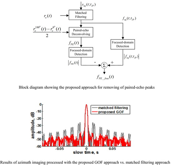
So far, however, there is no effective approach to eliminate such already existent “ghost targets” from strong scatterers caused by stair-step antenna steering in the process of SAR data imaging. It is found that by using amplitude tapering, there is a limited improvement for the reduction of the paired-echo peaks of IRF [2,10]. However, the use of azimuth tapering window is largely limited by the unwelcome loss of azimuth resolution. This paper aims at providing an approach implemented in SAR data processing, which can eliminate spurious peaks and restore an ideal IRF without resolution loss. Firstly, the amplitude modulated azimuth received signal is carefully modeled using the classic theory of paired echo distortion [6]. It is found that the undesired amplitude error caused by electronic beam steering cannot be determined in advance due to each target’s random jump time of beam angle, which will prevent the precise use of optimum filtering (OF) [16,17] to achieve an ideal IRF. Then an extended optimum filtering (EOF), which is originally proposed in [18] to remove the azimuth ambiguities in SAR images, is reintroduced here to accommodate the undetermined random modulation. However, it is found that EOF can only remove the strongest and nearest paired distortion peaks. To deal with this problem, the form of the ideal deconvolving filtering in EOF is reasonably approximated, and the limit of real receive signal basis is broken. A generalized optimum filtering (GOF) is then given. Using the proposed approach, not only the strongest and nearest paired distortion peaks, but also peripheral aliased power of the paired-echo-distorted IRF can be removed all together from the detected SAR images.

2. Paired Echoes Modeling

Assuming a sinc azimuth pattern and a continuous linear beam steering, the resulting TOPS antenna pattern as seen by a point target within its illumination time $T_{ap}$ is [2,8,9,10]:

$$\begin{array}{ll}{w}_o(t)& =G_0{\mathrm{sinc}}^2\left[\frac{L}{\lambda }\left(\frac{v}{R_0}t+k_{\psi }t\right)\right]\\ & =G_0{\mathrm{sinc}}^2\left[\frac{Lvt}{\lambda R_0}\cdot \left(1+\frac{R_0{k}_{\psi }}{v}\right)\right],t\in \left[-T_{ap}/2,T_{ap}/2\right]\end{array}$$

(1)

where $t$ represents the azimuth slow time referenced to this target’s beam center crossing, $k_{\psi }$ is the beam rotation rate, $L$ is the azimuth antenna length, $\lambda$ is the wavelength, $v$ is the ground velocity, and $R_0$ is the range of the closest approach. According to Equation (1), it is easy to know [2] that the TOPS azimuth resolution is reduced with respect to the stripmap resolution by a factor that is equal to:

$$\alpha =1+\frac{R_0{k}_{\psi }}{v}$$

(2)

which is always greater than 1. However, the real electronically-steered rotation angle versus the azimuth time shows typically a staircase behavior with a constant steering step period $T_Q$ [2,10]. Therefore, the practical antenna pattern should be rewritten as:

$$w_{aq}(t;t_{JP})=G_0{\mathrm{sinc}}^2\left\{\frac{L}{\lambda }\left[\frac{v}{R_0}t+k_{\psi }\left(\lfloor \frac{t-t_{JP}}{T_Q}\rfloor T_Q+\frac{T_Q}{2}+t_{JP}\right)\right]\right\},t\in \left[-T_{ap}/2,T_{ap}/2\right]$$

(3)

where $t_{JP}$ is the minimum slow-time jump point of rotation angle referenced to the target’s beam center crossing point, which is a uniformly distributed random variable within the range $\left(-T_Q/2,T_Q/2\right]$ for each different target and dependent on the target’s azimuth position, $\lfloor \ast \rfloor$ denotes the down-round operation. Note that the beam steering jumping happen at the same absolute slow-time points for all targets, however, a target with a randomly distributed azimuth position will have its own random absolute time of beam center crossing, therefore, $t_{JP}$, i.e., the closest jump point of beam steering referenced to the target’s beam center crossing, is a random value less than $T_Q/2$. Additionally, note that $T_Q/2$ is included in the round brackets so that the beam rotation angle is in accordance with the ideal continuous one at the center time of each electronically steering step. According to Equations (1)–(3), the practical antenna pattern $w_{aq}(t;t_{JP})$ can be further expressed as:

$$\begin{array}{ll}{w}_{aq}(t;t_{JP})& =G_0{\mathrm{sinc}}^2\left[\frac{Lv}{\lambda R_0}\left[\alpha t+\left(1-\alpha \right)\cdot \left(t-t_{JP}-\lfloor \frac{t-t_{JP}}{T_Q}\rfloor \cdot T_Q-\frac{T_Q}{2}\right)\right]\right]\\ & =w_o\left[t+\frac{1-\alpha }{\alpha }\cdot \xi (t-t_{JP})\right]\end{array}$$

(4)

where $\xi (t)$ is a periodic function with its period equaling the steering step period $T_Q$:

$$\xi (t)=t-\lfloor \frac{t}{T_Q}\rfloor \cdot T_Q-\frac{T_Q}{2}$$

(5)

It is well known that a periodic integrable function can be further expanded and expressed as the following Fourier series

$${\xi }^{fs}(t)\sim {\displaystyle \sum _{n=1}^{\infty }{a}_n\sin \left(\frac{2n\pi t}{T_Q}\right)}$$

(6)

where $a_n=-\frac{T_Q}{n\pi }$. According to Equations (5) and (6), it is known that $\left|\xi (t)\right|$ is always less than $T_Q/2$ and far less than the whole illumination time $T_{ap}$. On the other hand, the absolute value of the factor $\frac{1-\alpha }{\alpha }$ is always less than 1 according to Equation (2). In a word, $\frac{1-\alpha }{\alpha }\cdot \xi (t-t_{JP})$ is a quite short time frame, so that the following first-order Taylor expansion approximation is given:

$$\begin{array}{ll}{w}_{aq}(t;t_{JP})& \approx w_{aq}^{fs}(t;t_{JP})\\ & =w_o(t)+\frac{1-\alpha }{\alpha }{w}_o{}^{\prime }(t)\cdot {\xi }^{fs}(t-t_{JP})\\ & =w_o(t)+\frac{1-\alpha }{\alpha }{w}_o{}^{\prime }(t)\cdot {\displaystyle \sum _{n=1}^{\infty }{a}_n\sin \left(\frac{2n\pi (t-t_{JP})}{T_Q}\right)}\end{array}$$

(7)

where $w_o{}^{\prime }(t)$ represents the time derivation of $w_o(t)$. The accuracy of the approximation in Equation (7) will be checked in the simulation section of this paper. It is now clear that the antenna pattern with the effect of staircase-like beam steering shows a typical periodic amplitude modulation, and the sine terms in Equation (7) will lead to paired echoes in the IRF [6].

Now the antenna pattern weighted signal model will be derived. It is well known that SAR is a two-dimensional (2-D) system. However, for a typical TOPS mode, the 2-D frequency bandwidth is normally not wide, therefore the range-dimensional processing and range-azimuth decoupling are not closely related to the azimuth antenna pattern. For the sake of brevity, the azimuth one-dimensional (1-D) signal model is preferable for the following derivation [8,9,19]. The azimuth 1-D signal is the echo of one target after the first and secondary range compression (SRC), as well as the range cell migration (RCM) correction.

In a continuous linear beam steering case, after an azimuth demodulation step, called baseband azimuth scaling (BAS), integrated in the TOPS mode imaging processor [19,20], the echo from isolated target separated in azimuth is demodulated to zero Doppler centroid and can be represented without unnecessary terms as [8,9]:

$$s_o(t)=w_o\left(t\right)e^{-j\pi K_e{t}^2}$$

(8)

where $K_e$ is the effective azimuth chirp rate of the received signal [19]. In ideal conditions, the output focused signal after matched filtering is:

$$f_o(t)=s_o(t)\otimes r_a(t)=e^{j\pi K_e{t}^2}{\displaystyle {\int }_{-\infty }^{\infty }{w}_o(\tau )}{\mathrm{e}}^{-j2\pi K_{e}t\tau }d\tau =e^{j\pi K_e{t}^2}{W}_o\left(K_{e}t\right)$$

(9)

where $r_a(t)$ represents the ideal matched filter, and $W_o(\ast )$ is the Fourier transform of $w_o(t)$, representing the ideal IRF envelope. In contrast, in the step-by-step steering case, the received signal suffering an undesired amplitude modulation becomes:

$$s_{aq}(t;t_{JP})=w_{aq}(t){\mathrm{e}}^{-j\pi K_e{t}^2}=w_o\left[t+\frac{1-\alpha }{\alpha }\cdot \xi (t-t_{JP})\right]{\mathrm{e}}^{-j\pi K_e{t}^2}$$

(10)

According to the approximation given by Equation (7), $s_{aq}(t;t_{JP})$ can be approximated as $s_{aq}^{fs}(t;t_{JP})$:

$$\begin{array}{ll}{s}_{aq}^{fs}(t;t_{JP})& =w_{aq}^{fs}(t){\mathrm{e}}^{-j\pi K_e{t}^2}=\left[w_o(t)+\frac{1-\alpha }{\alpha }\cdot w_o{}^{\prime }(t)\cdot {\xi }^{fs}(t-t_{JP})\right]{\mathrm{e}}^{-j\pi K_e{t}^2}\\ & =\left[w_o(t)+\frac{1-\alpha }{\alpha }\cdot w_o{}^{\prime }(t)\cdot {\displaystyle \sum _{n=1}^{\infty }{a}_n\sin \left(\frac{2n\pi (t-t_{JP})}{T_Q}\right)}\right]{\mathrm{e}}^{-j\pi K_e{t}^2}\end{array}$$

(11)

If the same matched filtering in Equation (9) is used, the paired-echo-corrupted output signal can be expressed as follows if the Fourier series in Equation (6) is used and with reasonable approximation [6,8,9]:

$$\begin{array}{ll}{f}_{aq}(t;t_{JP})& =s_{aq}(t;t_{JP})\otimes r_a(t)\\ & \approx f_o(t)+{\displaystyle \sum _{n=1}^{\infty }{A}_n}\left[e^{-jn{\varphi }_{JP}}\cdot \left(t-n{T}_d\right)\cdot f_o(t-n{T}_d)-e^{jn{\varphi }_{JP}}\cdot \left(t+n{T}_d\right)\cdot f_o(t+n{T}_d)\right]\end{array}$$

(12)

where:

$$T_d=\frac{1}{K_e{T}_Q}$$

(13)

is a time parameter representing an azimuth time displacement, and the amplitude coefficient is:

$$A_n=\frac{1-\alpha }{\alpha }\pi K_e{a}_n{e}^{j\pi K_e{n}^2{T}_{{}_d}^2}$$

(14)

and:

$${\varphi }_{JP}=2\pi \frac{t_{JP}}{T_Q}$$

(15)

is a $\left(-\pi ,\pi \right]$ uniformly distributed random phase determined by the target’s azimuth-time jump point $t_{JP}$, which is further dependent on the azimuth target position. Note that Equation (11) is similar to the signal model given in [8] and [9], however, the random phase ${\varphi }_{JP}$ is neglected in [8,9]. It also should be noted that the existence of the amplitude terms $\left(t\pm n{T}_d\right)$ will lead to a peak splitting for those paired-echo distortion peaks.

3. Paired Echoes Elimination

3.1. Optimum Filtering and its Extension Approach

By a comparison of Equation (10) versus Equation (8), it is clear that there exists unavoidable amplitude error in Equation (10), which has caused undesired paired-echo peaks in the focused domain given by Equation (12). According to the basic concept of the OF [16] (optimum filter, otherwise called the ideal filter [17]), if a precise knowledge of the amplitude error in Equation (10) is available, an optimum filter can be generated. It is a reference function for SAR azimuth processing which provides, in addition to the matched filtering for the received signal, the deconvolution of the amplitude error according to the a priori knowledge about it.

For instance, suppose that it is known in advance that the azimuth-time jump point $t_{JP}$ of one target is zero, i.e., ${\varphi }_{JP}=0°$, the amplitude-distorted received echo $s_{aq}^{0°}(t)$ can then be predicted according to Equation (10):

$$s_{aq}^{0°}(t)\triangleq s_{aq}\left(t;t_{JP}=0\right)=w_o\left[t+\frac{1-\alpha }{\alpha }\cdot \xi (t)\right]{\mathrm{e}}^{-j\pi K_e{t}^2}$$

(16)

and a corresponding ideal deconvolving filter $r_c^{0°}(t)$ can be defined using $s_{aq}^{0°}(t)$. It can be more conveniently expressed in the frequency domain as $R_c^{0°}(f)$ by the following equation:

$$R_c^{0°}(f)=\frac{S_o(f)}{S_{aq}^{0°}(f)}$$

(17)

It is obvious that the ideal deconvolving filter given in Equation (17) can accurately eliminate the amplitude error in the received signal from targets with zero azimuth-time jump point, so that with an additional matched filtering, an ideal IRF will be obtained. This will be verified by the simulation in Section 4 (see the ideal output from the matched 0° OF path of the EOF approach).

In another example, if we know that another target’s $t_{JP}$ value is $T_Q/2$, i.e., ${\varphi }_{JP}=180°$ according to (15), then the amplitude-distorted echo $s_{aq}^{180°}(t)$ can be given according to Equation (10):

$$s_{aq}^{180°}(t)\triangleq s_{aq}\left(t;t_{JP}=\frac{T_Q}{2}\right)=w_o\left[t+\frac{1-\alpha }{\alpha }\cdot \xi \left(t-\frac{T_Q}{2}\right)\right]\cdot {\mathrm{e}}^{-j\pi K_e{t}^2}$$

(18)

and using the corresponding ideal deconvolving filter $R_c^{180°}(f)$, defined as:

$$R_c^{180°}(f)=\frac{S_o(f)}{S_{aq}^{180°}(f)}$$

(19)

the amplitude error in the echoes from targets with azimuth-time jump point $t_{JP}=T_Q/2$ will be accurately deconvolved so as to achieve an ideal IRF. This will also be verified by the simulation in Section 4 (see the ideal output from the matched 180° OF path of the EOF approach).

The above two examples show how the conventional OF works. Unfortunately, as analyzed in Section 2, the absolute phase value ${\varphi }_{JP}$ for a random distributed target cannot be determined in advance due to the target’s undetermined azimuth-time jump point $t_{JP}$. Therefore, the conventional idea of OF will fail to deal with all targets separated in azimuth with different random positions.

In order to solve this problem, the extended OF method (EOF), which is originally proposed in [18] to remove the azimuth ambiguities in SAR images, will be reintroduced here to accommodate the undetermined random modulation. In [18], by modeling the insufficiently sampled azimuth discrete signal, it is found that the absolute phase $\Delta {\varphi }_a$ of the azimuth ambiguities cannot be determined due to the fractional sampling shift $\delta x$. Although the way that modeling azimuth ambiguity is quite different from the way in this paper, in that neither the theory of paired echo distortion nor other series-expansion approximation is necessary [18], the relationship between the absolute phase $\Delta {\varphi }_a$ and fractional sampling shift $\delta x$ in [18] is very similar to the relationship between the absolute phase ${\varphi }_{JP}$ and $t_{JP}$ established in Section 2.

In order to handle the undefined phase of the azimuth ambiguities in [18], the single-chain-path filtering of the conventional OF approach is extended and a dual-path filtering approach, i.e., EOF, is proposed [18], in which two deconvolving functions corresponding to zero and half a sampling interval for the fractional shift $\delta x$ are generated respectively. In a similar way described in [18], besides the ideal deconvolving function for $t_{JP}=0$ given by Equations (16) and (17), the additional ideal deconvolving function for $t_{JP}=T_Q/2$ at half a steering period is also generated according to Equations (18) and (19). The two OF processing paths then can produce two images which have the main peak signal in phase but the principal aliased signal out of phase [18]. The corresponding two OF processing paths can be represented as:

$$f_{ideal}^{0°}(t)=s_{aq}(t;t_{JP})\otimes r_c^{0°}(t)\otimes r_a(t)$$

(20)

$$f_{ideal}^{180°}(t)=s_{aq}(t;t_{JP})\otimes r_c^{180°}(t)\otimes r_a(t)$$

(21)

The subtraction of $f_{ideal}^{180°}(t)$ from $f_{ideal}^{0°}(t)$ will eliminate the main peak of IRF, since it has the same phase in both case. After detection and division by 2 of the result of subtraction [18], we obtain the paired echo image:

$$\left|f_{PE}^{}(t)\right|=\frac{1}{2}\left|f_{ideal}^{180°}(t)-f_{ideal}^{0°}(t)\right|$$

(22)

Then, by subtracting $f_{PE}^{}(t)$ from the image $\left|f_{aq}(t;t_{JP})\right|$ given by Equation (12), which is generated with conventional matched filtering, the ultimate image which is free from the paired echoes can be obtained:

$$f_{PE\_free}(t)=\left|f_{aq}(t)\right|-\left|f_{PE}^{}(t)\right|$$

(23)

Since the convolution operations in Equations (20) and (21) are linear, which satisfy combination and distributive laws, in order to simplify computing, the two OF processing paths can be combined, the following block diagram in Figure 1 is used to realize the EOF approach.

3.2. Generalized Optimum Filtering

It is pointed out in [18] that the EOF approach with the defined two deconvolving functions can efficiently suppress the first ambiguities of point targets, however, the second ambiguities cannot be suppressed simultaneously with the same deconvolving functions. It is mentioned that new deconvolving-function pairs (e.g., a different combination of $\delta x$ values) are needed to be defined in order to specially suppress the second ambiguities if necessary. Since, for the use of azimuth ambiguity suppression in [18], normally only the first azimuth ambiguities are strong enough and likely to become “ghost targets”, the suppression of second ambiguities is often not necessary and, therefore, not further investigated in [18].

Similarly, in the simulation given in the following Section 4, it will be found that the EOF approach given in the Section 3.1 will face the same issue. It can remove the strongest paired distortion peaks in the distorted IRF well, however, the peripheral aliased power of the paired-echo-distorted IRF (esp. the second-strongest components) cannot be effectively eliminated. Though the used ideal deconvolving filters defined by Equations (16)–(19) are generated based on the accurate signal model given by Equation (10), here it is helpful for the understanding of the above not-so-good results if we keep the paired-echo-distortion model in Equations (11) and (12) under observation. According to Equations (12) and (15), we can find that a change of half a steering stepping period in the $t_{JP}$ value (from $t_{JP}=0$ in Equation (16) to $t_{JP}=T_Q/2$ in Equation (18)) will rotate the phase of the aliased paired echo signal by $n\cdot \pi$. It means the phase rotation angle is dependent on the paired echo number n. For the first-strongest aliased paired peaks (n = 1), the rotated phase is $\pi$, which means a phase reversion between the two OF paths; however, for the second-strongest aliased paired peaks (n = 2), the rotated phase is $2\pi$, representing an in-phase performance between the two OF paths. The main peak signal of the IRF also has in-phase performance between the two OF paths. Therefore, it is easy to understand that the second-strongest aliased paired peaks will be preserved in the ultimate image just like the main peak signal be done.

According to Equation (14), the second-strongest paired echoes may be only a few dBs lower than the strongest aliased peaks, so that in this paper, an improved procedure must be developed to simultaneously consider both the strongest paired distortion peaks and the peripheral aliased power of the paired echoes. The solution can be found if we break through the traditional limit on the OF concept that the ideal deconvolving function must be generated based on the physically received distorted signal, as Equations (17) and (19) have fulfilled.

In the following, two generalized received echoes, $s_{aq,gof}^{0°}(t)$ and $s_{aq,gof}^{180°}(t)$ are defined as substitutes of $s_{aq}^{0°}(t)=s_{aq}\left(t;t_{JP}=0\right)$ (see Equation (16)) and $s_{aq}^{180°}(t)=s_{aq}\left(t;t_{JP}=\frac{T_Q}{2}\right)$ (see Equation (18)), respectively:

$$\begin{array}{ll}{s}_{aq,gof}^{0°}(t)& ={\left[w_o(t)+\frac{1-\alpha }{\alpha }\cdot w_o{}^{\prime }(t)\cdot {\xi }^{fs}(t-t_{JP})\right]|}_{t_{JP}=0}\times {\mathrm{e}}^{-j\pi K_e{t}^2}\\ & =\left[w_o(t)+\frac{1-\alpha }{\alpha }\cdot w_o{}^{\prime }(t)\cdot {\displaystyle \sum _{n=1}^{\infty }{a}_n\sin \left(\frac{2n\pi t}{T_Q}\right)}\right]\times {\mathrm{e}}^{-j\pi K_e{t}^2}\end{array}$$

(24)

$$s_{aq,gof}^{180°}(t)=\left[w_o(t)+\frac{1-\alpha }{\alpha }\cdot w_o{}^{\prime }(t)\cdot {\displaystyle \sum _{n=1}^{\infty }{a}_n\sin \left(\frac{2n\pi t}{T_Q}+\pi \right)}\right]\times {\mathrm{e}}^{-j\pi K_e{t}^2}$$

(25)

In actual application, the order n will be reasonably limited by a maximum value of N. It is found that $s_{aq,gof}^{0°}(t)$ is generated according to $s_{aq}^{fs}(t;t_{JP}=0)$ given by Equation (11), and still can be regarded as the approximation version of $s_{aq}^{0°}(t)$. However, $s_{aq,gof}^{180°}(t)$ no longer corresponds with any real $t_{JP}$ value. In other words, $s_{aq,gof}^{180°}(t)$ is utterly artificial “echo”. Nevertheless, it can be found that the phase of paired-echo terms in $s_{aq,gof}^{180°}(t)$ are all offset to the phase of the corresponding ones in $s_{aq,gof}^{0°}(t)$ by 180°. Then, in the same way shown in Equations (17) and (19), two new “ideal” deconvolving filters, $R_{c,gof}^{0°}(f)=\frac{S_o(f)}{S_{aq,gof}^{0°}(f)}$ and $R_{c,gof}^{180°}(f)=\frac{S_o(f)}{S_{aq,gof}^{180°}(f)}$, can be generated using the defined function $s_{aq,gof}^{0°}(t)$ and $s_{aq,gof}^{180°}(t)$. What calls for special attention is that since $s_{aq,gof}^{0°}(t)$ is only the approximation of the real echo $s_{aq}^{0°}(t)$, and more importantly $s_{aq,gof}^{180°}(t)$ is an utterly artificial echo, $R_{c,gof}^{0°}(f)$ and $R_{c,gof}^{180°}(f)$ are actually beyond the traditional concept of ideal deconvolving filtering in OF or EOF. In other words, neither $R_{c,gof}^{0°}(f)$ or $R_{c,gof}^{180°}(f)$ can ideally eliminate the amplitude error in the received signal from any real targets. This declaration will be verified by the simulation in Section 4 (see the non-ideal IFRs from either OF path of the GOF approach). Therefore, here we call $R_{c,gof}^{0°}(f)$ and $R_{c,gof}^{180°}(f)$ generalized deconvolving filter (GDF). Now using the new pair of GDF, in a same way shown in Equations (20) and (21), the output of two generalized OF paths for arbitrary target echo $s_{aq}(t;t_{JP})$ becomes:

$$\begin{array}{ll}{f}_{gof}^{0°}(t)& =s_{aq}(t;t_{JP})\otimes r_{c,gof}^{0°}(t)\otimes r_a(t)\\ & =f_o(t)-2{\displaystyle \sum _{n=1}^{\infty }\sin \left(\frac{n{\varphi }_{JP}}{2}\right)A_n}\left[e^{j\left(-\frac{n{\varphi }_{JP}}{2}+\frac{\pi }{2}\right)}\cdot \left(t-n{T}_d\right)\cdot f_o(t-n{T}_d)+e^{j\left(\frac{n{\varphi }_{JP}}{2}+\frac{\pi }{2}\right)}\cdot \left(t+n{T}_d\right)\cdot f_o(t+n{T}_d)\right]\end{array}$$

(26)

$$\begin{array}{ll}{f}_{gof}^{180°}(t)& =s_{aq}(t;t_{JP})\otimes r_{c,gof}^{180°}(t)\otimes r_a(t)\\ & =f_o(t)+2{\displaystyle \sum _{n=1}^{\infty }\cos \left(\frac{n{\varphi }_{JP}}{2}\right)A_n}\left[e^{-j\frac{n{\varphi }_{JP}}{2}}\cdot \left(t-n{T}_d\right)\cdot f_o(t-n{T}_d)-e^{j\frac{n{\varphi }_{JP}}{2}}\cdot \left(t+n{T}_d\right)\cdot f_o(t+n{T}_d)\right]\end{array}$$

(27)

By comparing above two equations, it is found that the two OF paths produce two images $f_{gof}^{0°}(t)$ and $f_{gof}^{180°}(t)$, which have the main peak signal in phase but all the symmetrically displaced paired-echo distortion signal in quadrature. Then the subtraction of $f_{gof}^{180°}(t)$ from $f_{gof}^{0°}(t)$ will result in the following paired echo image represented as:

$$\begin{array}{ll}{f}_{PE}^{gof}(t)& =\frac{1}{2}\left|f_{gof}^{180°}(t)-f_{gof}^{0°}(t)\right|\\ & ={\displaystyle \sum _{n=1}^{\infty }\left|A_n\right|}\cdot \left\{\left|\left(t-n{T}_d\right)\cdot f_o(t-n{T}_d)\right|+\left|\left(t+n{T}_d\right)\cdot f_o(t+n{T}_d)\right|\right\}\end{array}$$

(28)

The ultimate paired-echo-free image can then be obtained:

$$f_{PE\_free}^{gof}(t)=\left|f_{aq}(t)\right|-\left|f_{PE}^{gof}(t)\right|=\left|f_o(t)\right|$$

(29)

The new result no longer contains the peripheral aliased power of the paired-echo-distorted IRF. It is clear that the new GOF approach shares the same processing flow chart of the EOF approach shown in Figure 1, the only necessary modification is replacing $r_c^{180°}(t)$ and $r_c^{0°}(t)$ with $r_{c,gof}^{180°}(t)$ and $r_{c,gof}^{0°}(t)$, respectively. Note that using the GOF or EOF approach in this paper, the IRF amplitude is well preserved, however, the phase information is lost due to the focused-domain detection operation shown in Figure 1, the same case occurs in the ambiguity suppression processing in [18].

4. Simulation Results

Simulations are performed in this section. All the simulations are based on the multi-mode version of SBRAS (Space-borne Radar Advance Simulator) [21,22]. This multi-mode simulator supports the parameter design, raw data simulation, data focusing and performance evaluation of strip-map mode, sliding spotlight mode, TOPS mode, and so on [21]. The implementation of this simulator for spaceborne SAR modes with azimuth beam steering could be found in [20], [23,24,25]. The designed parameters used in the simulation are listed in

Table 1. List of simulation parameters.

Parameters	Value
Transmit wavelength	0.054 m
Target distance	680 km
Azimuth resolution	20 m
Mean steering rate	1.73°/s
Antenna length	10 m
Mean look angle	35°
Transmit chirp bandwidth	10 MHz
Rotation angle stepping period	0.02 s/0.03 s

, the TOPS mode raw data are simulated assuming a C-band spaceborne system with an azimuth resolution of 20 m and a beam steering rate $k_{\psi }$ = 1.73°/s. The main steering stepping period $T_Q$ is 0.02 s, the corresponding angle stepping size of about 0.035°, which is a little larger than the stepping size of 0.03° chosen in the design of TerraSAR mode [2,10]. An alternative choice of $T_Q$ = 0.03 s (0.052° of angle stepping size) is also investigated, which is designed under the applied background of low-cost spaceborne SAR payloads.

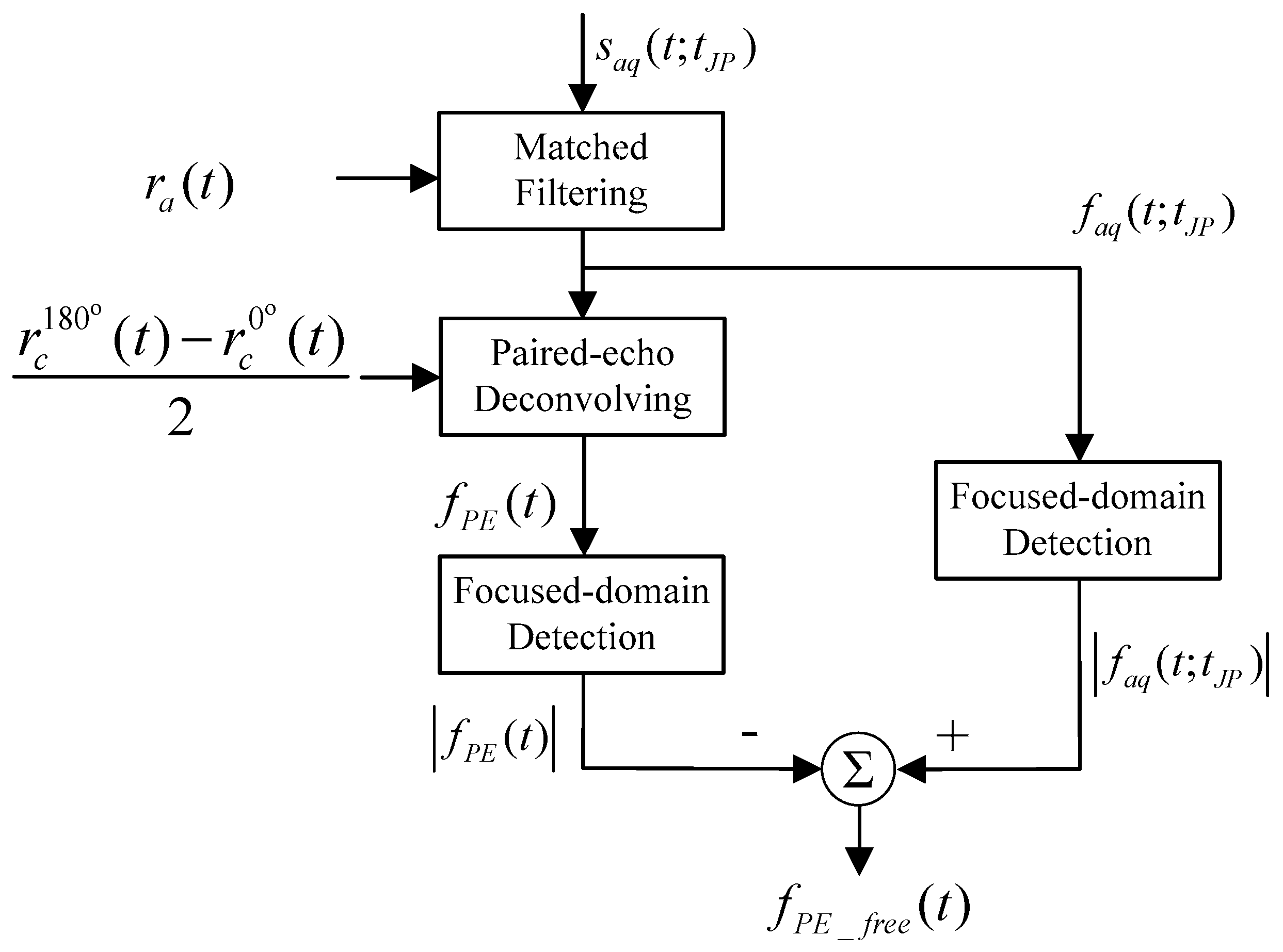
The effects of the staircase-like antenna steering to two-way antenna pattern seen by a target with the designed TOPS mode are shown in Figure 2. The solid red line represents the case $T_Q$ = 0.02 s and the solid gray line represents the case $T_Q$ = 0.03 s. As a contrast, the ideal TOPS mode two-way antenna pattern with a continuous beam steering is also given by the grey dotted line. Here the beam steering jump point $t_{JP}$ is randomly set as $0.3467\times \frac{T_Q}{2}$. It is found that the results in Figure 2 are similar to the simulated TOPS antenna gain shown in Figure 3 of [2].

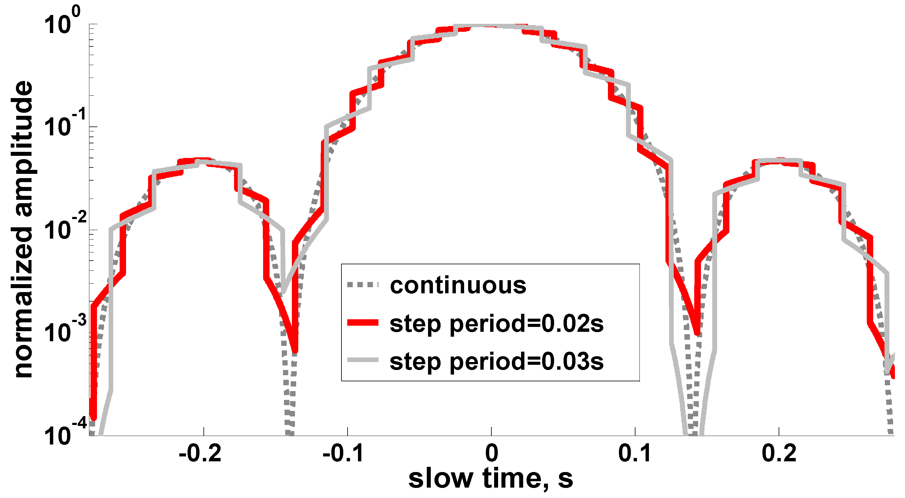
The undesired amplitude modulation caused by staircase-like steering in the raw data of a point target is represented by the difference between the ideal and the staircase antenna gain. The normalized amplitude differences of the above two antenna patterns with different stepping size are shown in Figure 3, which is like a saw tooth signal, as analyzed in [2]. The jump points of beam steering can be found clearly in this figure. It also can be seen that a larger stepping angle size will enlarge the undesired amplitude modulation.

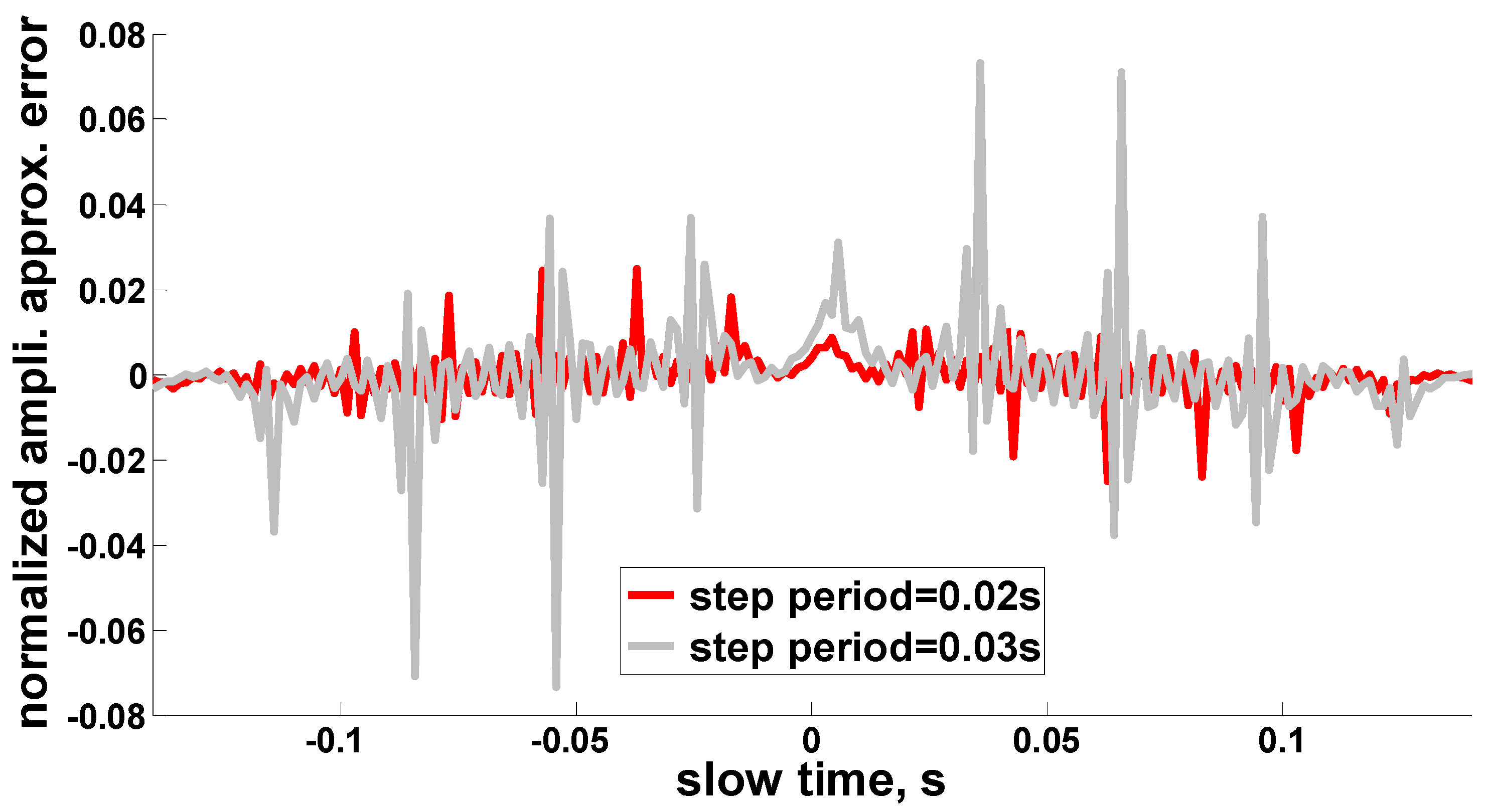
The approximation errors for the two antenna patterns using the approximate antenna pattern model given by Equation (7) are also shown in Figure 4. The Fourier series expansion number N is set to 6. It can be seen that the approximations perform well for both cases, i.e., $T_Q$ = 0.02 s and $T_Q$ = 0.03 s. It is also found that the approximation errors are relatively larger around the jump points of beam steering.

In order to verify the performance of the EOF and the proposed GOF approach for targets separated in azimuth with different azimuth position, Figure 5, Figure 6 and Figure 7 show the azimuth focusing processing results of three point targets at different azimuth positions in the imaged scene. The steering step period $T_Q$ is equal to 0.02 s for Figure 5, Figure 6 and Figure 7. For GOF approach, the Fourier series expansion number is set as N = 6 uniformly.

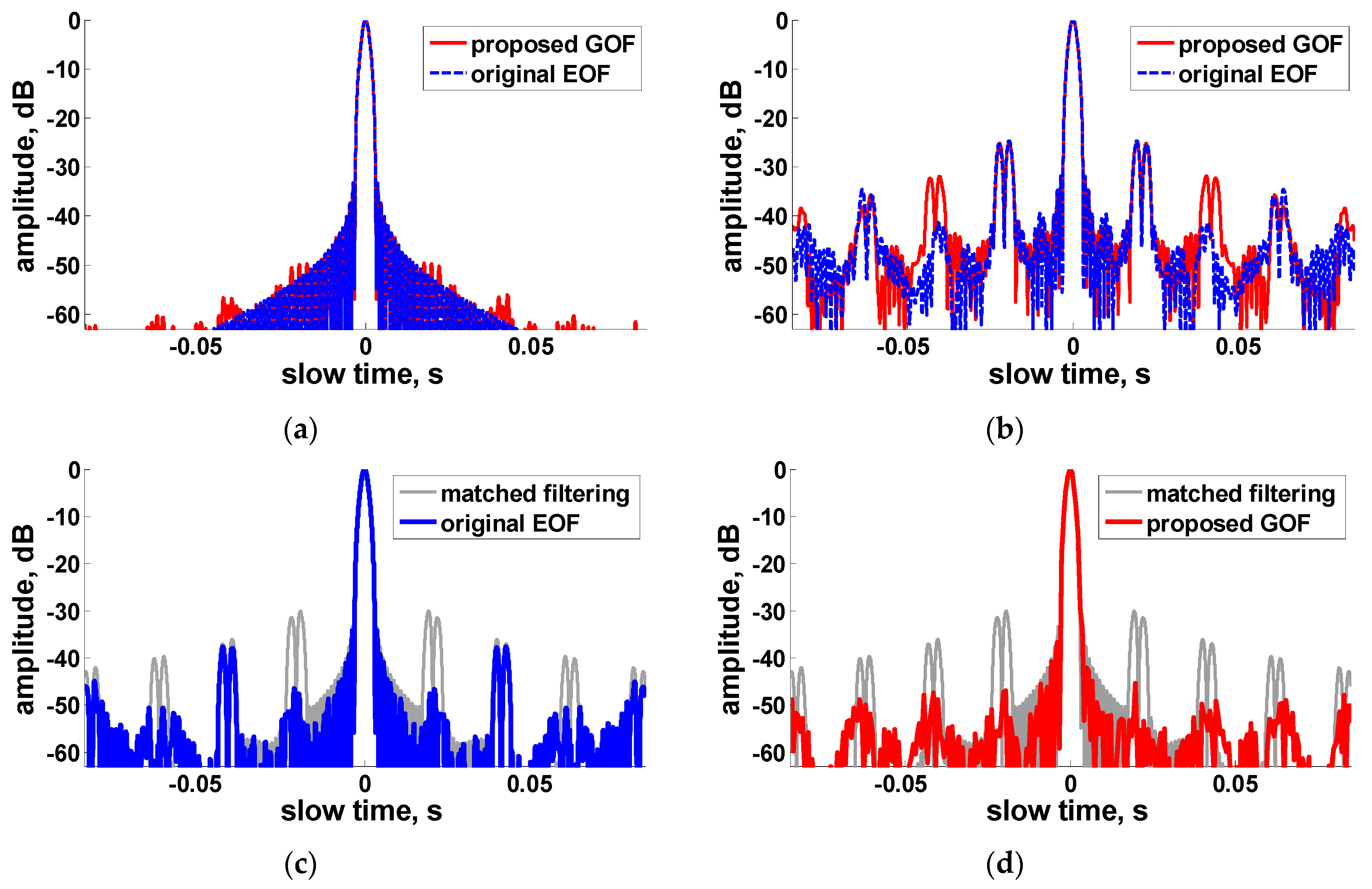
In Figure 5, the azimuth position of the tested target is chosen purposively so that the azimuth-time jump point $t_{JP}$ = 0, corresponding to ${\varphi }_{JP}=0°$ (see Equation (15)). Figure 5a shows the first OF-path output of EOF and GOF approaches. For the EOF approach, since the first path is predefined for $t_{JP}$ = 0, the correct $t_{JP}$ value is actually met in this path, therefore, an ideal IRF is obtained as shown in the blue lines. For the GOF approach, however, since the first-path filtering is only an approximation of OF for $t_{JP}$ = 0, only a nearly ideal IRF is obtained, as shown in the red lines. Figure 5b shows the second OF-path output of EOF and GOF approaches, which is predefined for $t_{JP}$ = $T_Q/2$ (${\varphi }_{JP}=180°$) in the EOF approach. 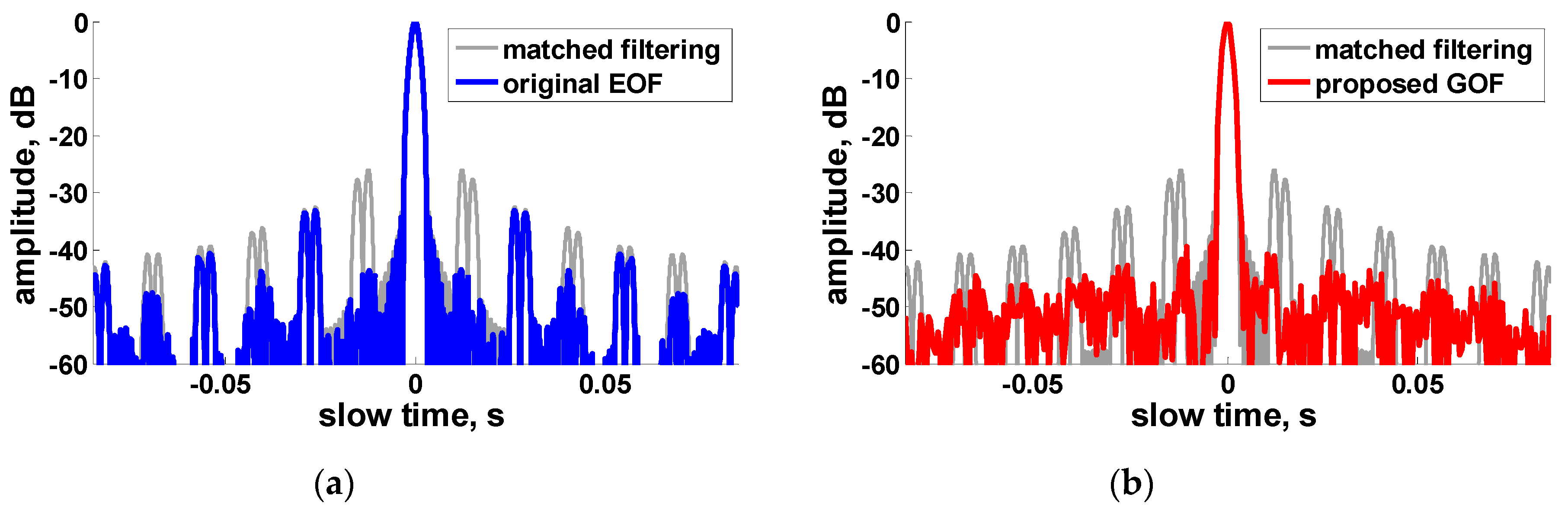For both approaches, the “ideal” deconvolution filtering is out of operation due to the mismatched information about $t_{JP}$, however, the output of GOF contains more useful paired-echo information, which can be used to cancel the paired echoes in the matched filtering output (see the gray lines in Figure 5c,d). The ultimate results of both approaches are shown in (c) and (d) in contrast to the matched filtering result, respectively. It can be seen that the EOF approach can efficiently suppress the strongest paired echoes, however, due to the unsuccessful suppression for the second-strongest paired echoes, the output paired-echo peak ratio of the IRF is still about −37 dB. For the result of GOF approach, both the strongest paired distortion peaks and the peripheral power of the distorted IRF can be satisfactorily suppressed, the overall amplitude level of the paired echoes is about −49 dB.

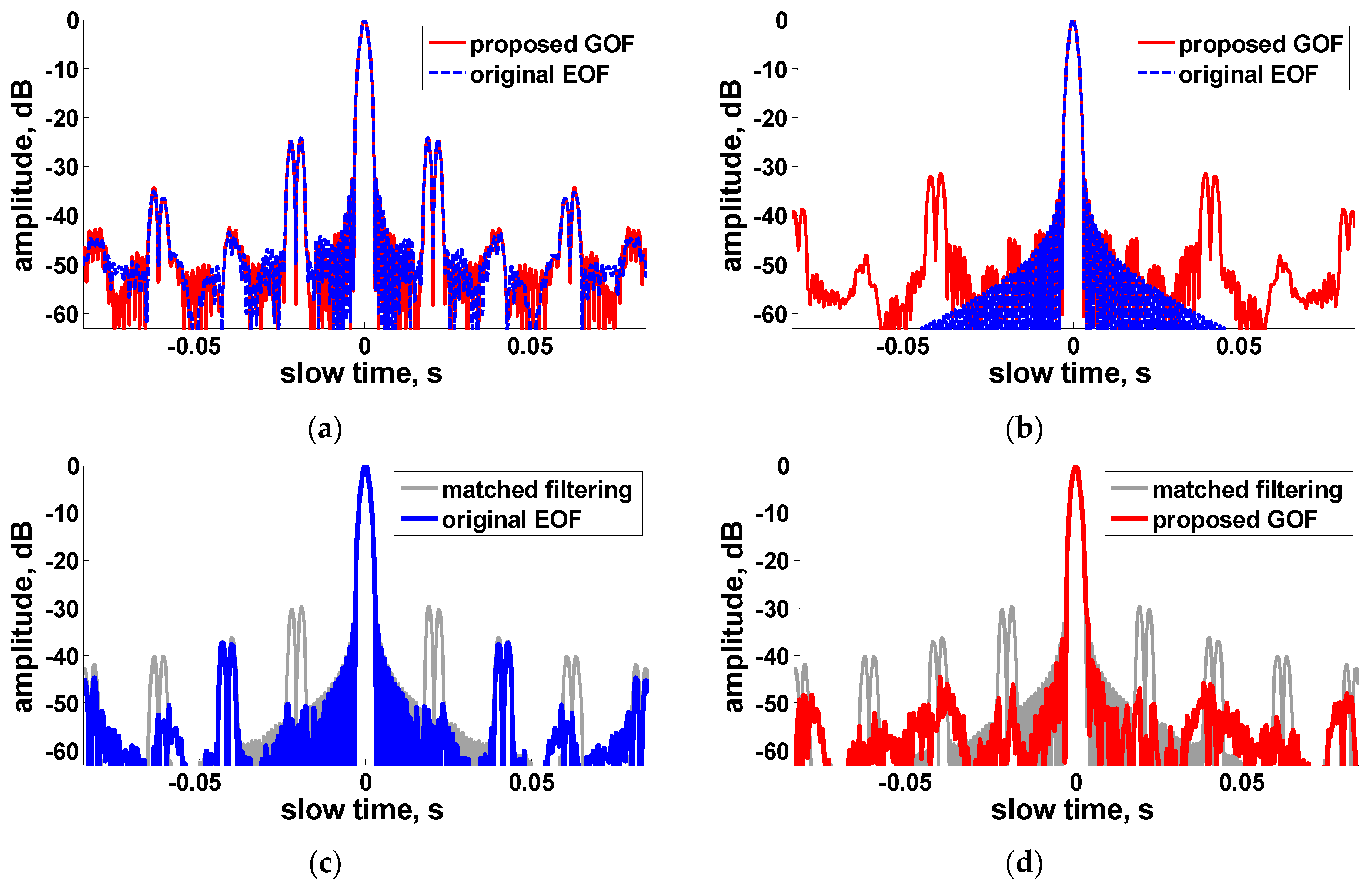
In Figure 6, the azimuth position of the tested target is changed so that the azimuth-time jump point $t_{JP}=T_Q/2$, corresponding to ${\varphi }_{JP}=180°$. Now note that in Figure 6b, since the second path is predefined for $t_{JP}=T_Q/2$, this time the correct $t_{JP}$ value is met in the second path, therefore, an ideal IRF is obtained in the second OF-path as shown in the blue line. On the contrary, the second OF-path output of GOF approach shown in red line is far from an ideal IRF (in contrast to the nearly ideal IRF from the first OF-path of GOF in a matched $t_{JP}$ case, show in red lines in Figure 5a), and this demonstrates the fact that the second OF-path of GOF is more special and is generated based on a physically nonexistent artificial “echo”. The ultimate processing results for both EOF and GOF are quite similar to the results shown in Figure 5.

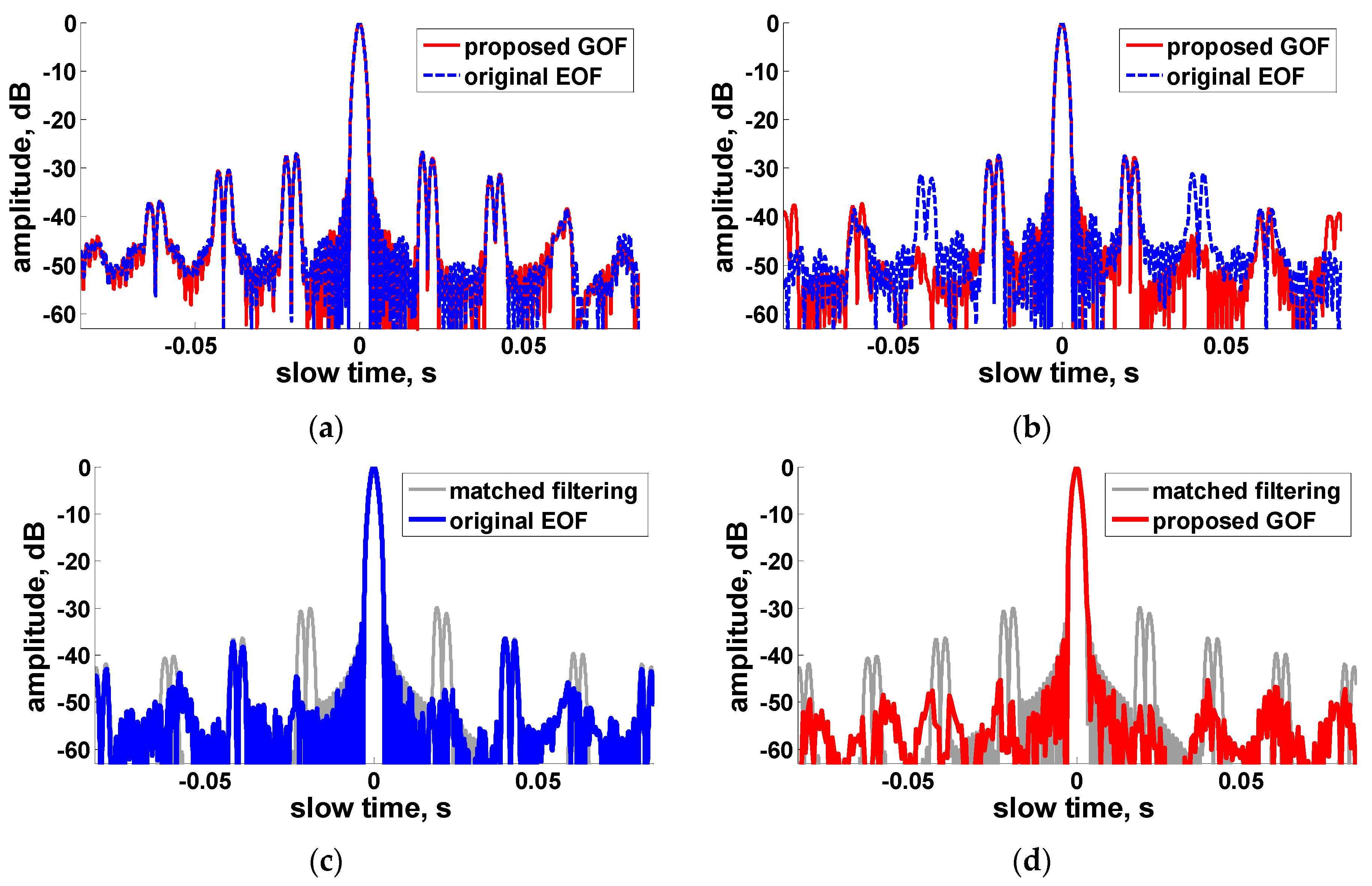
In Figure 7, now the azimuth position of the tested target is set to make the azimuth-time jump point $t_{JP}$ equal to $0.5\times (T_Q/2)$. In some sense, this is the worst case for optimum matched filtering, since the real $t_{JP}$ is in the center of $\left[0,T_Q/2\right]$, it means now the real echo is close to neither of the two OF-paths. Nevertheless, we still obtain very similar ultimate results for EOF and GOF.

Overall, from the results shown in Figure 5, Figure 6 and Figure 7, it is observed that, although the second OF-path output of GOF approach is never near an ideal IRF for any one of the three targets, the combined processing with the first OF-path will obtain a satisfactory result for both suppression of the strongest paired peaks and the peripheral power of the distorted IRF. Both the performance of GOF and EOF are stable and not dependent on the target azimuth position. The original paired echo peak ratio for match filtering is −30 dB ($T_Q$ = 0.02 s), after the proposed GOF approach, the peak ratio is not exceed −48 dB; after the EOF approach, the peak ratio is not exceed −37 dB.

In Figure 8, the processing results in the case that $T_Q$ = 0.03 s is given. It is found that with a larger angle step size, the paired echo peak ratio for conventional match filtering is about −25 dB, which is much higher than the case when $T_Q$ = 0.02 s. The peak ratio of the GOF result is below −40 dB, while the peak ratio of the EOF result is below −32 dB.

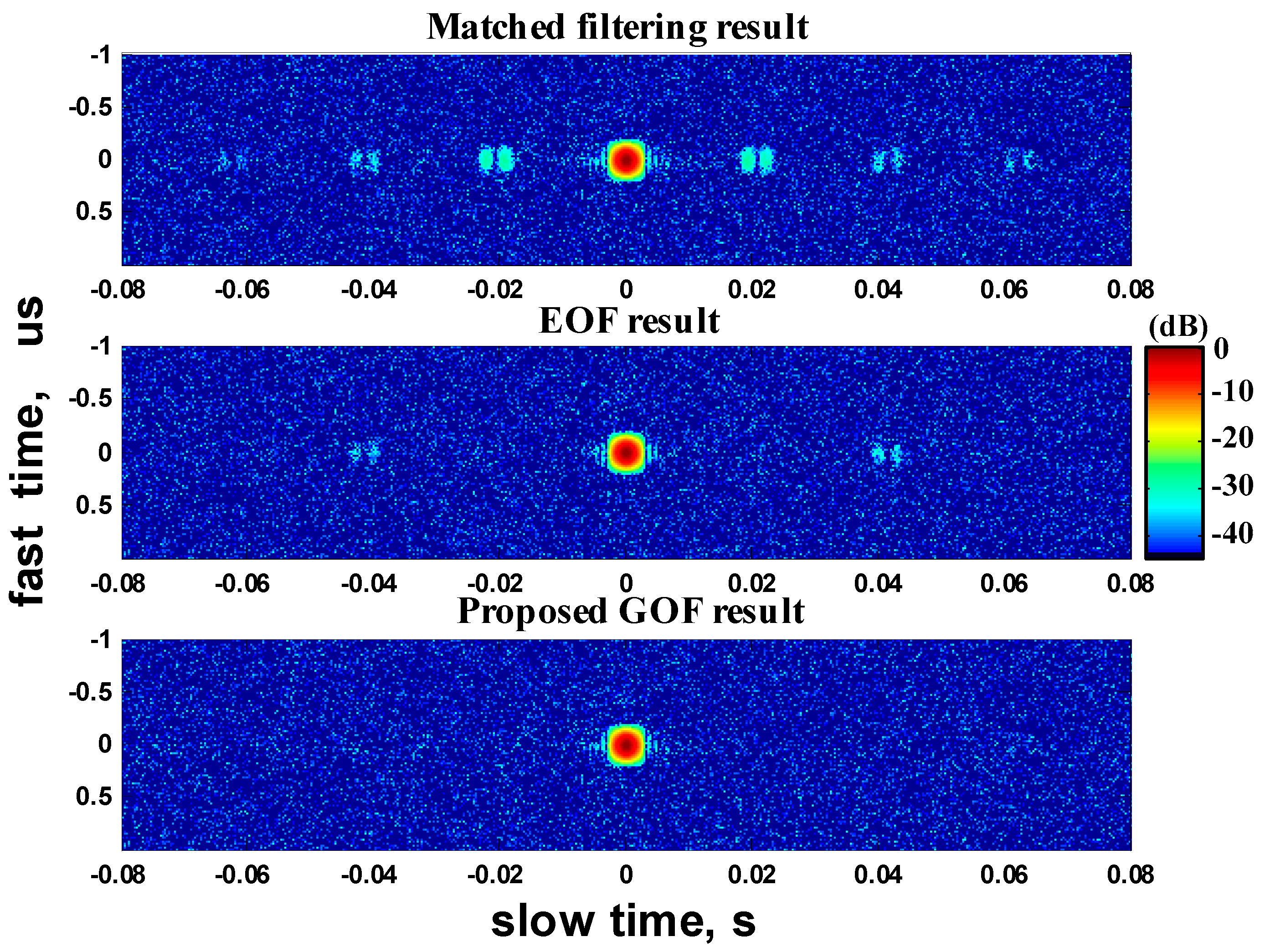
The azimuth 1-D simulation above is quite essential for showing the detailed processing results suited to quantitative analysis. Since SAR imaging is actually a 2-D process, the 2-D processing results are also simulated and given in Figure 9; Figure 10. This time nine strong point targets having different range and azimuth positions are evenly embedded in a 6 km × 6 km scene of low backscatter. They are arranged in such a way that the targets in the corner positions limit the 6 km × 6 km scene in the azimuth and range, respectively. It is found that all the nine targets have the similar processing performance. Figure 9 and Figure 10 show the results of two targets located at the top left corner and bottom right corner of the scene, respectively. It is found that “ghost targets” from strong point targets embedded in a scene of low backscatters in the process of conventional SAR data imaging are eliminated if the data are processed with the proposed GOF approach. However, if the data are processed with the EOF approach, there are still remnant “ghost targets”.

5. Discussion

It is found that the proposed GOF approach and the EOF approach given in [18] share the same processing flow. The main difference between GOF and EOF is the way how to generate two OF paths. The two OF paths of EOF approach are made up of two conventional deconvolving filters generated according to the accurate signal model given by Equation (10), corresponding to two different given beam steering jump point $t_{JP}$ values, and no approximation in Equations (7) and (11) regarding paired-echo-distortion modeling is needed in the generation of the deconvolving functions. The IRFs plotted in blue in Figure 5a and Figure 6b have shown that perfect IRF can be achieved from one individual OF path among the two EOF paths if the correct $t_{JP}$ value is actually met. The two OF paths of GOF approach, however, cannot be regarded as conventional ideal deconvolving filters. The IRFs plotted in red in the subimages (a) and (b) of Figure 5, Figure 6 andFigure 7 have shown that no perfect IRF can be achieved from any individual OF path among the two GOF paths. In this sense, GOF is a new reasonable approximation of the EOF approach originally proposed in [18], and, in theory, EOF can obtain better single-path performance than GOF.

Nevertheless, it is found from the ultimate results that by the combination use of the two OP paths, GOF approach can achieve better suppression on the paired echo peaks than the EOF approach, esp. for the second-strongest aliased paired peaks. The GOF approach performs stably and azimuth independently in all of the simulation cases. In the case that $T_Q$ = 0.02 s, the paired echo peak ratio can be suppressed from −30 dB to a level of about −50 dB; In the case that $T_Q$ = 0.03 s, the peak ratio is suppressed from −25 dB to a level of −40 dB. For the EOF approach, however, the peak ratios are −37 dB and −32 dB for $T_Q$ = 0.02 s and $T_Q$ = 0.03 s, respectively.

In addition, a series truncation in Equations (24) and (25) is required for the GOF approach. Increasing the Fourier series expansion number can improve accuracy of the antenna pattern approximation model. Since the two-path filter functions would be pre-calculated and then can be used for the batch processing of images acquired with the same steering mode, a larger series expansion number will not increase on-line computation load. Based on these considerations, in the simulation, the series expansion number N is uniformly set as 6.

6. Conclusions

The use of electronically-steered antennas leads to a staircase-like antenna beam steering law in the TOPS wide-swath imaging mode, which will introduce paired echoes in the IRF, thus “ghost targets” may appear in the focused images for strong isolated scatterers. This paper proposes a new approach to suppress such already existing “ghost targets” based on the extended optimum filtering approach [18] and the approximation and generalization of the ideal deconvolving filtering included in the approach. In the simulation with raw data from a C-band TOPS SAR mode with a staircase-like steering, it is found that the proposed approach can well suppress paired echoes from strong point-like targets in a scene of low backscatter.