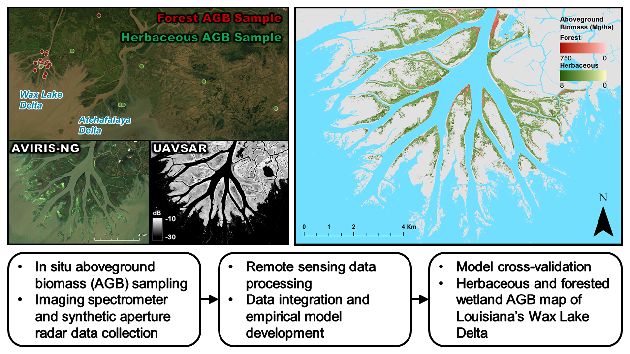
Integrating Imaging Spectrometer and Synthetic Aperture Radar Data for Estimating Wetland Vegetation Aboveground Biomass in Coastal Louisiana

 , , ,
, , ,
Abstract
:
1. Introduction
2. Materials and Methods
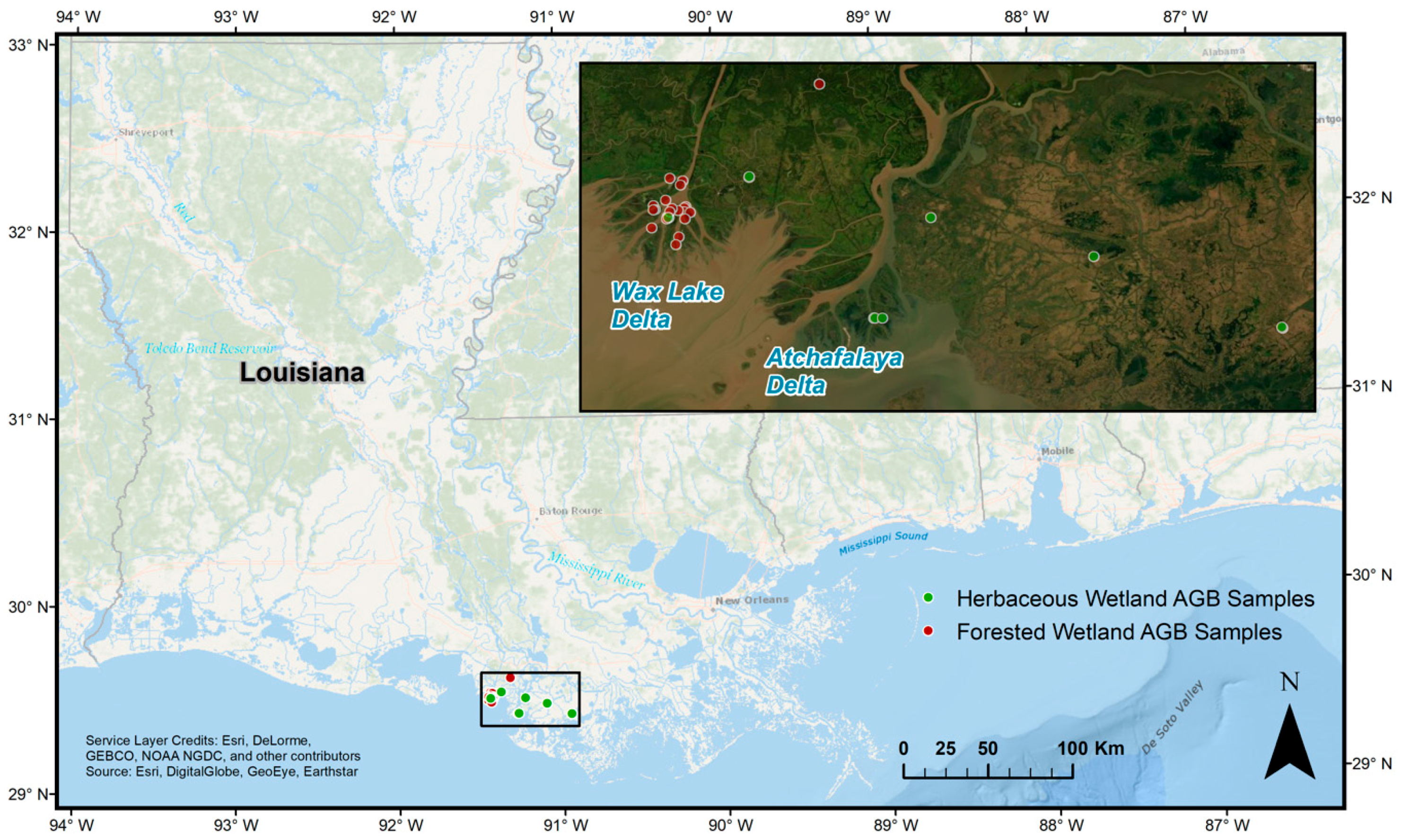
2.1. Field Data
2.2. Remote Sensing Data
2.2.1. Imaging Spectrometer Data
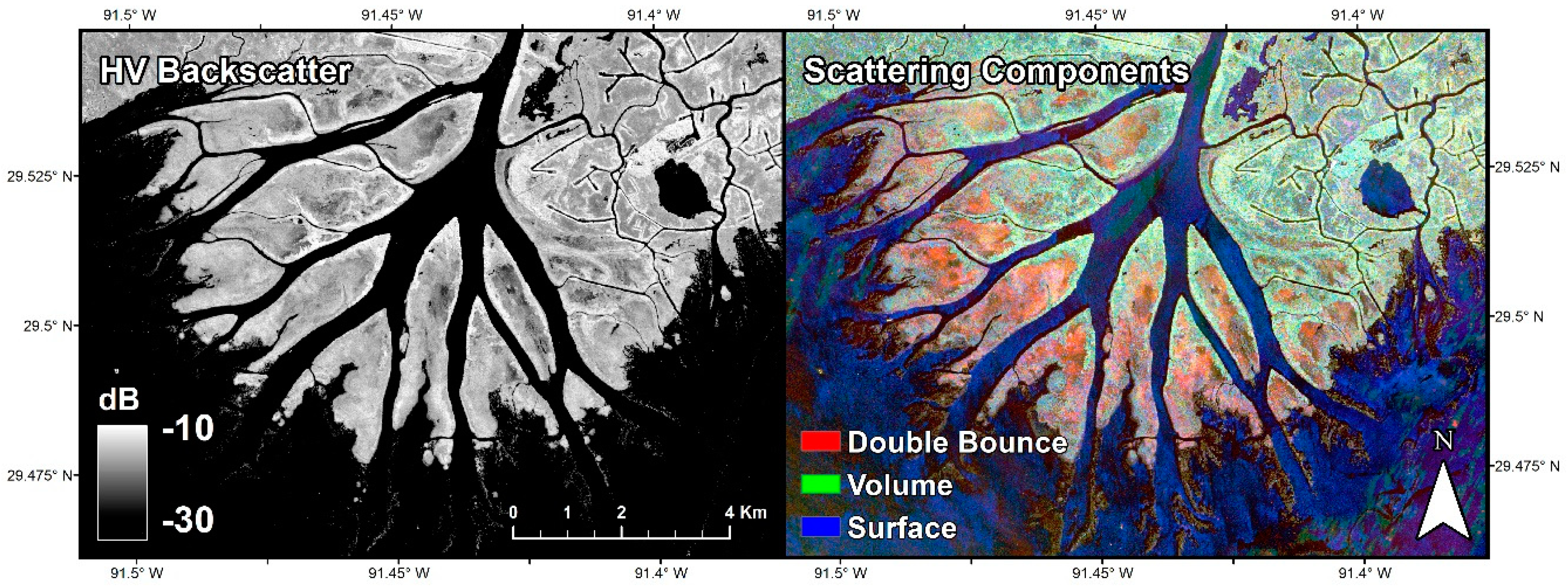
2.2.2. Synthetic Aperture Radar Data
2.3. Model Development
2.3.1. Single Sensor Ordinary Least Squares Regression Models
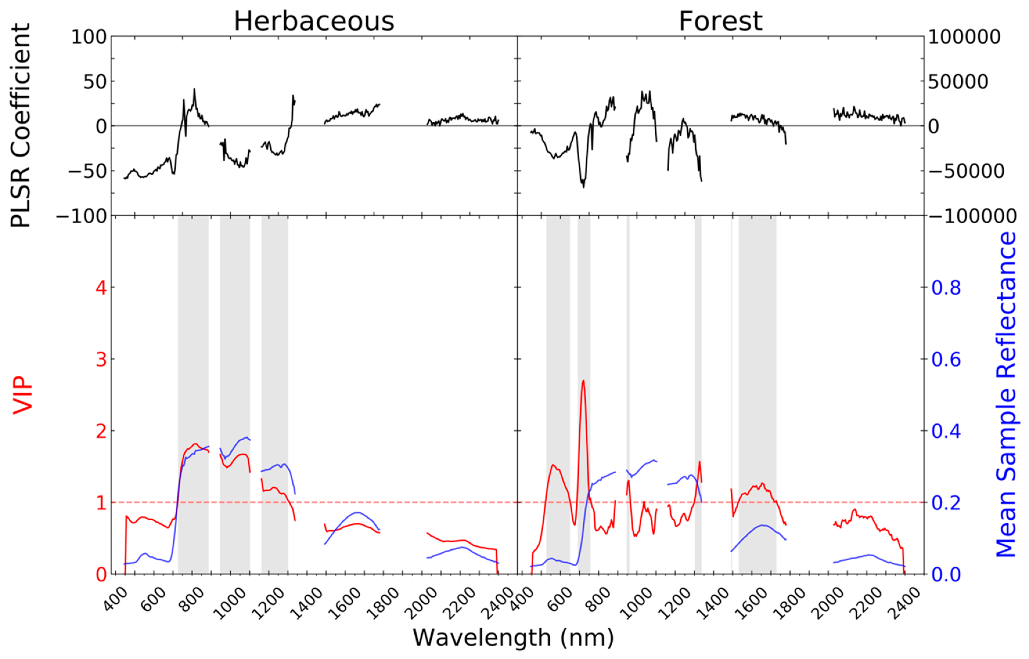
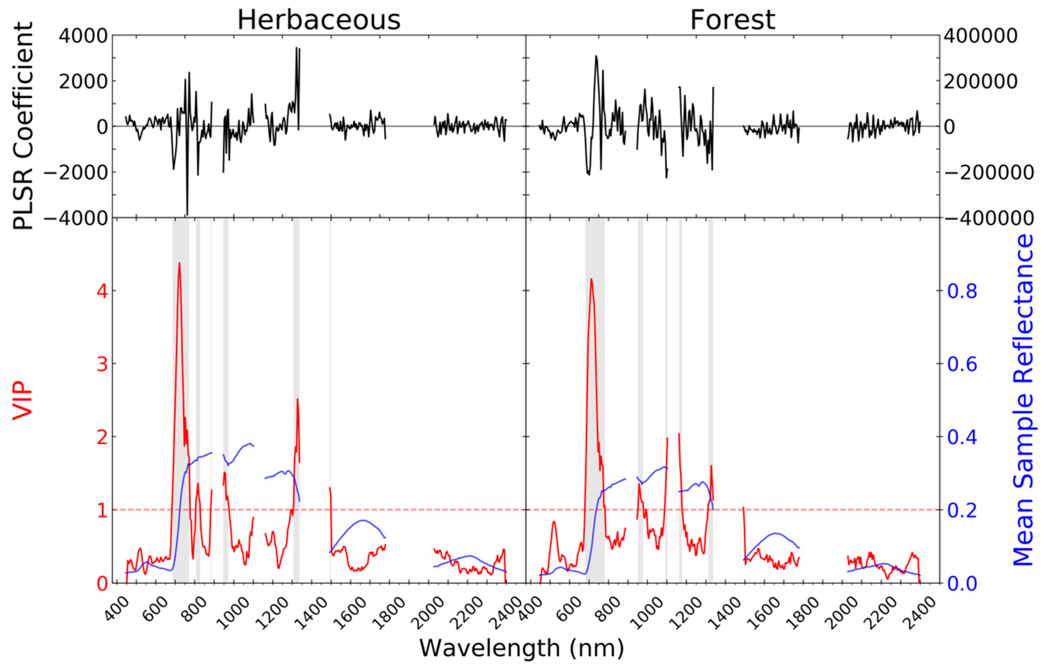
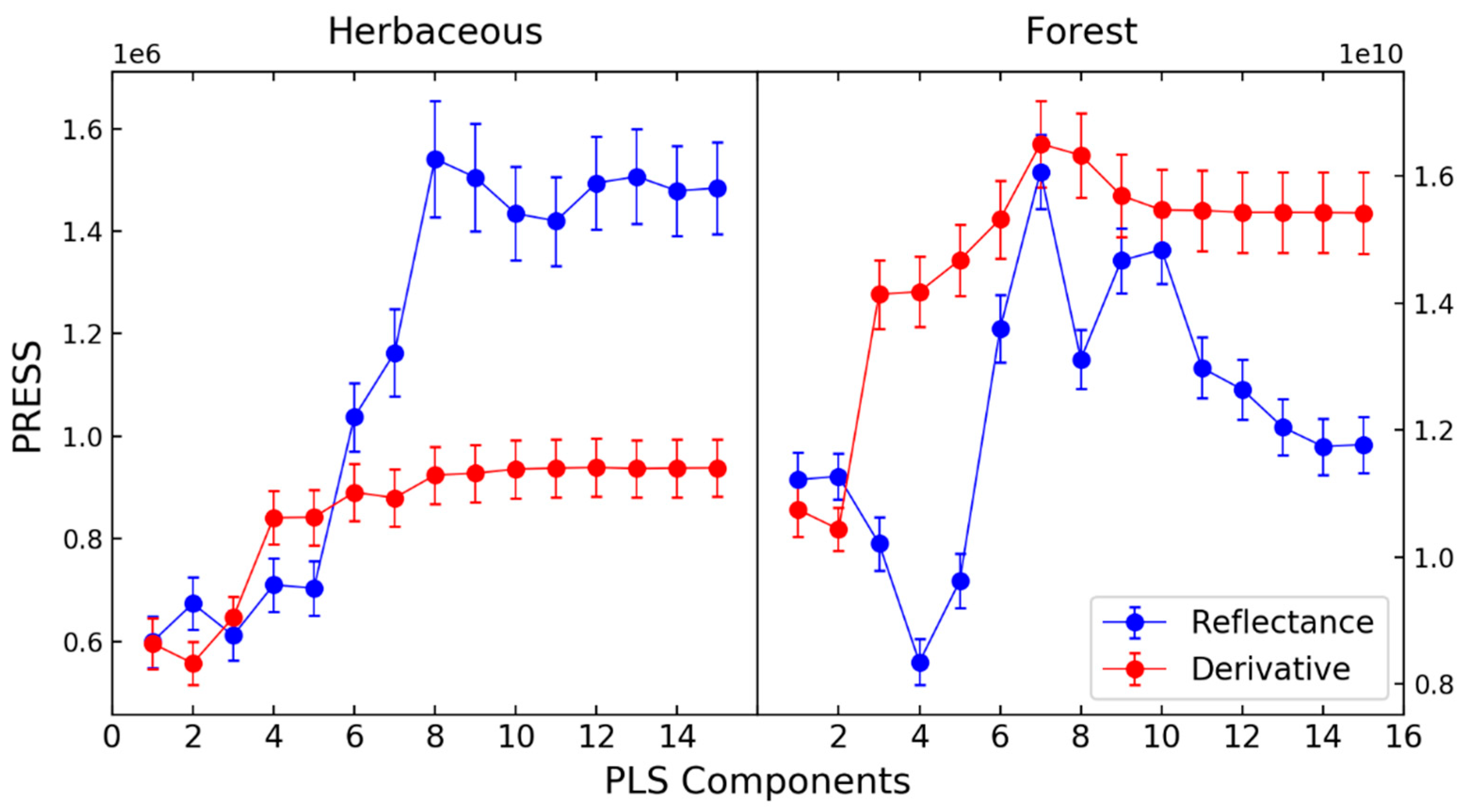
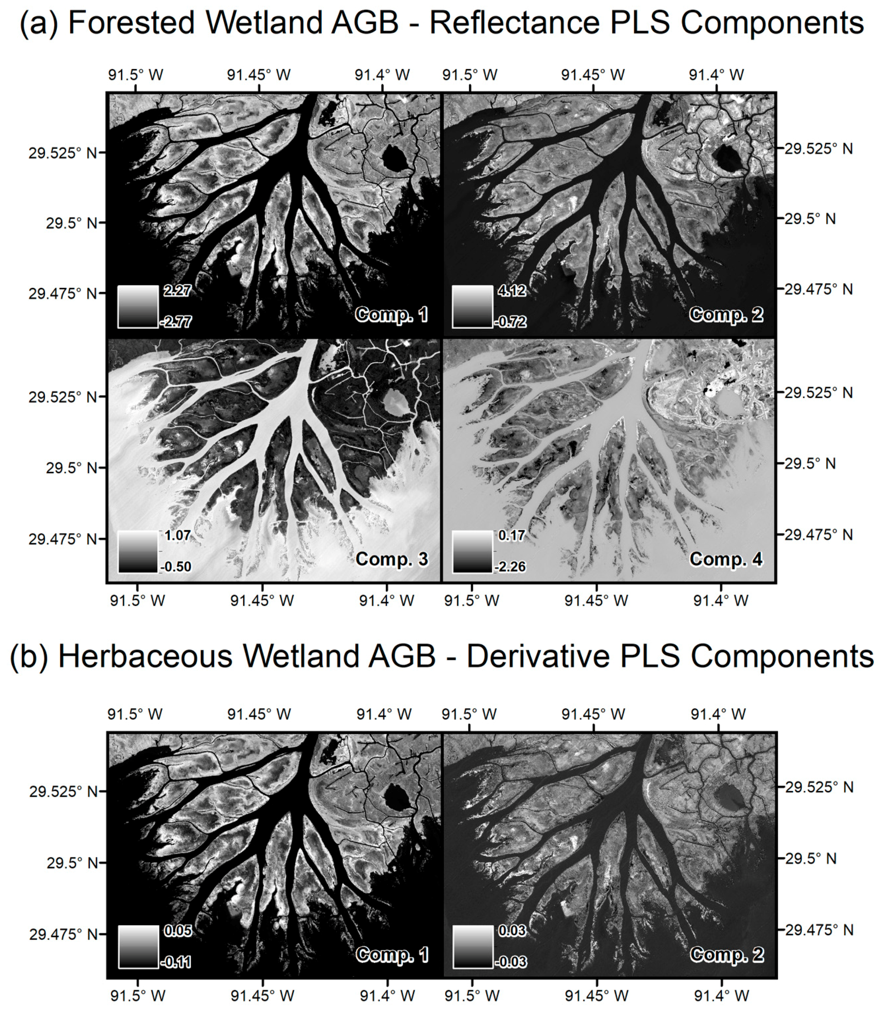
2.3.2. Imaging Spectrometer Partial Least Squares Regression Models
2.3.3. Integrated Multi-Sensor Models
3. Results
4. Discussion
5. Conclusions
Author Contributions
Funding
Acknowledgments
Conflicts of Interest
Appendix A

| Collection Date | Plot Size (m2) | Latitude | Longitude | Dominant Species | AGB (g/m2) |
|---|---|---|---|---|---|
| 6 May 2015 | 0.25 | 29.53893 | −91.38042 | Sagittaria lancifolia | 324.10 |
| 6 May 2015 | 0.25 | 29.53918 | −91.38051 | Sagittaria lancifolia | 401.52 |
| 6 May 2015 | 0.25 | 29.53943 | −91.38044 | Sagittaria lancifolia | 394.42 |
| 8 May 2015 | 0.25 | 29.42521 | −91.27973 | Alternanthera philoxeroides | 132.92 |
| 8 May 2015 | 0.25 | 29.47480 | −91.10216 | Spartina alterniflora | 332.30 |
| 8 May 2015 | 0.25 | 29.42525 | −91.27923 | Ludwigia grandiflora | 259.50 |
| 8 May 2015 | 0.25 | 29.42533 | −91.27925 | Typha domingensis | 299.20 |
| 8 May 2015 | 0.25 | 29.42527 | −91.27888 | Typha domingensis | 519.10 |
| 8 May 2015 | 0.25 | 29.42527 | −91.27280 | Colocasia esculenta | 244.44 |
| 8 May 2015 | 0.25 | 29.50637 | −91.23360 | Saururus cernuus | 126.00 |
| 9 May 2015 | 0.25 | 29.41716 | −90.94989 | Sagittaria lancifolia | 451.28 |
| 9 May 2015 | 0.25 | 29.41719 | −90.94984 | Eleocharis radicans | 338.00 |
| 9 May 2015 | 0.25 | 29.41759 | −90.95010 | Sagittaria lancifolia | 908.76 |
| 9 May 2015 | 0.25 | 29.41762 | −90.95002 | Sagittaria lancifolia | 622.20 |
| 9 May 2015 | 0.25 | 29.41796 | −90.95036 | Sagittaria lancifolia | 379.44 |
| 15 November 2016 | 0.25 | 29.50650 | −91.44556 | Colocasia esculenta | 250.04 |
| 15 November 2016 | 0.25 | 29.50644 | −91.44558 | Colocasia esculenta | 351.44 |
| 15 November 2016 | 0.25 | 29.50639 | −91.44567 | Colocasia esculenta | 253.72 |
| 15 November 2016 | 0.25 | 29.50672 | −91.44564 | Colocasia esculenta | 243.32 |
| 15 November 2016 | 0.25 | 29.50664 | −91.44550 | Colocasia esculenta | 279.68 |
| 15 November 2016 | 0.49 | 29.50664 | −91.44539 | Colocasia esculenta | 482.02 |
| 15 November 2016 | 0.49 | 29.50656 | −91.44542 | Colocasia esculenta | 348.67 |
| 15 November 2016 | 0.75 | 29.50639 | −91.44541 | Colocasia esculenta | 255.73 |
| 15 November 2016 | 0.75 | 29.50647 | −91.44531 | Colocasia esculenta | 380.67 |
| 15 November 2016 | 0.75 | 29.50655 | −91.44576 | Colocasia esculenta | 402.40 |
| Collection Date | Plot Radius (m) | Latitude | Longitude | Dominant Species | AGB (g/m2) |
|---|---|---|---|---|---|
| 6–8 May 2015 | 10 | 29.51538 | −91.43171 | Salix nigra | 38,030 |
| 6–8 May 2015 | 10 | 29.51121 | −91.43267 | Salix nigra | 8160 |
| 6–8 May 2015 | 10 | 29.51070 | −91.42787 | Salix nigra | 42,590 |
| 6–8 May 2015 | 10 | 29.50545 | −91.43219 | Salix nigra | 30,100 |
| 6–8 May 2015 | 10 | 29.61462 | −91.32393 | Taxodium distichum | 19,552 |
| 6–8 May 2015 | 10 | 29.49074 | −91.43710 | Salix nigra | 8850 |
| 6–8 May 2015 | 10 | 29.61431 | −91.32350 | Salix nigra | 1790 |
| 6–8 May 2015 | 10 | 29.51413 | −91.43279 | Salix nigra | 51,520 |
| 6–8 May 2015 | 10 | 29.51214 | −91.43756 | Salix nigra | 23,100 |
| 6–8 May 2015 | 10 | 29.51361 | −91.44246 | Salix nigra | 16,350 |
| 6–8 May 2015 | 10 | 29.51607 | −91.45768 | Salix nigra | 13.830 |
| 6–8 May 2015 | 10 | 29.51266 | −91.45770 | Salix nigra | 30,210 |
| 6–8 May 2015 | 10 | 29.50539 | −91.44698 | Salix nigra | 3070 |
| 6–8 May 2015 | 10 | 29.53821 | −91.44451 | Salix nigra | 36,300 |
| 6–8 May 2015 | 10 | 29.53608 | −91.43400 | Salix nigra | 66,080 |
| 6–8 May 2015 | 10 | 29.53263 | −91.43570 | Salix nigra | 34,780 |
| 6–8 May 2015 | 10 | 29.50715 | −91.44643 | Salix nigra | 5180 |
| 6–8 May 2015 | 10 | 29.53821 | −91.44451 | Salix nigra | 36,300 |
| 6–8 May 2015 | 10 | 29.53608 | −91.43400 | Salix nigra | 66,080 |
| 6–8 May 2015 | 10 | 29.53263 | −91.43570 | Salix nigra | 34,780 |
| 6–8 May 2015 | 10 | 29.51538 | −91.43171 | Salix nigra | 38,030 |
| 6–8 May 2015 | 10 | 29.51413 | −91.43279 | Salix nigra | 51,520 |
| 6–8 May 2015 | 10 | 29.51121 | −91.43267 | Salix nigra | 8160 |
| 6–8 May 2015 | 10 | 29.51070 | −91.42787 | Salix nigra | 42,590 |
| 6–8 May 2015 | 10 | 29.51214 | −91.43756 | Salix nigra | 23,100 |
| 6–8 May 2015 | 10 | 29.51361 | −91.44246 | Salix nigra | 16,350 |
| 6–8 May 2015 | 10 | 29.51607 | −91.45768 | Salix nigra | 13,830 |
| 6–8 May 2015 | 10 | 29.51299 | −91.45649 | Salix nigra | 16,710 |
| 6–8 May 2015 | 10 | 29.52044 | −91.44769 | Salix nigra | 29,990 |
| 6–8 May 2015 | 10 | 29.49821 | −91.45908 | Salix nigra | 24,020 |
| 6–8 May 2015 | 10 | 29.51266 | −91.45770 | Salix nigra | 30,210 |
| 6–8 May 2015 | 10 | 29.50545 | −91.43219 | Salix nigra | 30,100 |
| 6–8 May 2015 | 10 | 29.50539 | −91.44698 | Salix nigra | 3070 |
| 6–8 May 2015 | 10 | 29.49074 | −91.43710 | Salix nigra | 8850 |
| 6–8 May 2015 | 10 | 29.48458 | −91.43940 | Salix nigra | 10,430 |
| 6–8 May 2015 | 10 | 29.51120 | −91.44429 | Salix nigra | 6370 |
| Herbaceous Model Coefficient | Forest Model Coefficient | |
|---|---|---|
| Derivative PLS Component 1 | −1966.287 | |
| Derivative PLS Component 2 | −11555.016 | |
| Reflectance PLS Component 1 | 1188.786 | |
| Reflectance PLS Component 2 | −16,737.491 | |
| Reflectance PLS Component 3 | −194,039.813 | |
| Reflectance PLS Component 4 | −41,831.015 | |
| Volume Scattering Component | −7.293 | 1471.021 |
| Double Bounce Scattering Component | 3.418 | −1398.494 |
| Constant | 339.758 | 23,568.644 |
References
- Zhang, M.; Ustin, S.L.; Rejmankova, E.; Sanderson, E.W. Monitoring Pacific Coast Salt Marshes Using Remote Sensing. Ecol. Appl. 1997, 7, 1039–1053. [Google Scholar] [CrossRef]
- Morris, J.T.; Sundareshwar, P.V.; Nietch, C.T.; Kjerfve, B.; Cahoon, D.R. Responses of Coastal Wetlands to Rising Sea Level. Ecology 2002, 83, 2869–2877. [Google Scholar] [CrossRef]
- Mudd, S.M.; Howell, S.M.; Morris, J.T. Impact of dynamic feedbacks between sedimentation, sea-level rise, and biomass production on near-surface marsh stratigraphy and carbon accumulation. Estuar. Coast. Shelf Sci. 2009, 82, 377–389. [Google Scholar] [CrossRef]
- Adam, E.; Mutanga, O.; Rugege, D. Multispectral and hyperspectral remote sensing for identification and mapping of wetland vegetation: A review. Wetl. Ecol. Manag. 2010, 18, 281–296. [Google Scholar] [CrossRef]
- Byrd, K.B.; O’Connell, J.L.; Di Tommaso, S.; Kelly, M. Evaluation of sensor types and environmental controls on mapping biomass of coastal marsh emergent vegetation. Remote Sens. Environ. 2014, 149, 166–180. [Google Scholar] [CrossRef]
- Thomas, N.; Simard, M.; Cateñeda-Moya, E.; Byrd, K.; Windham-Myers, L.; Bevington, A.; Twilley, R.R. High-resolution mapping of biomass and distribution of marsh and forested wetlands in southeastern coastal Louisiana. Int. J. Appl. Earth Obs. Geoinf. 2019, 80, 257–267. [Google Scholar] [CrossRef]
- Craft, C.; Clough, J.; Ehman, J.; Jove, S.; Park, R.; Pennings, S.; Guo, H.; Machmuller, M. Forecasting the effects of accelerated sea-level rise on tidal marsh ecosystem services. Front. Ecol. Environ. 2009, 7, 73–78. [Google Scholar] [CrossRef] [Green Version]
- Kirwan, M.L.; Guntenspergen, G.R. Influence of tidal range on the stability of coastal marshland. J. Geophys. Res. 2010, 115, 1–11. [Google Scholar] [CrossRef]
- Turpie, K.R.; Klemas, V.V.; Byrd, K.; Kelly, M.; Jo, Y.H. Prospective HyspIRI global observations of tidal wetlands. Remote Sens. Environ. 2015, 167, 206–217. [Google Scholar] [CrossRef] [Green Version]
- Schile, L.M.; Callaway, J.C.; Morris, J.T.; Stralberg, D.; Thomas Parker, V.; Kelly, M. Modeling tidal marsh distribution with sea-level rise: Evaluating the role of vegetation, sediment, and upland habitat in marsh resiliency. PLoS ONE 2014, 9, e88760. [Google Scholar] [CrossRef]
- Rouse, J.W.; Hass, R.H.; Schell, J.A.; Deering, D.W. Monitoring vegetation systems in the great plains with ERTS. In Proceedings of the Third Earth Resources Technology Satellite (ERTS) Symposium, Washington, DC, 10–14 December 1973; Volume 1, pp. 309–317. [Google Scholar]
- Li, X.; Gar-On Yeh, A.; Wang, S.; Liu, K.; Liu, X.; Qian, J.; Chen, X. Regression and analytical models for estimating mangrove wetland biomass in South China using Radarsat images. Int. J. Remote Sens. 2007, 28, 5567–5582. [Google Scholar] [CrossRef]
- Klemas, V. Remote Sensing of Coastal Wetland Biomass: An Overview. J. Coast. Res. 2013, 290, 1016–1028. [Google Scholar] [CrossRef]
- Hong, S.H.; Wdowinski, S. Double-bounce component in cross-polarimetric SAR from a new scattering target decomposition. IEEE Trans. Geosci. Remote Sens. 2014, 52, 3039–3051. [Google Scholar] [CrossRef]
- Elvidge, C.D.; Chen, Z. Comparison of broad-band and narrow-band red and near-infrared vegetation indices. Remote Sens. Environ. 1995, 54, 38–48. [Google Scholar] [CrossRef]
- Townsend, P.A.; Foster, J.R.; Chastian, R.A., Jr.; Currie, W.S. Canopy nitrogen in the forests of the Central Appalachian Mountains using Hyperion and AVIRIS. IEEE Trans. Geosci. Remote Sens. 2003, 41, 1347–1354. [Google Scholar] [CrossRef]
- Townsend, P.A.; Serbin, S.P.; Kruger, E.L.; Gamon, J.A. Disentangling the contribution of biological and physical properties of leaves and canopies in imaging spectroscopy data. Proc. Natl. Acad. Sci. USA 2013, 110, E1074. [Google Scholar] [CrossRef]
- Cho, M.A.; Skidmore, A.; Corsi, F.; van Wieren, S.E.; Sobhan, I. Estimation of green grass/herb biomass from airborne hyperspectral imagery using spectral indices and partial least squares regression. Int. J. Appl. Earth Obs. Geoinf. 2007, 9, 414–424. [Google Scholar] [CrossRef]
- Tsai, F.; Philpot, W. Derivative analysis of hyperspectral data. Remote Sens. Environ. 1998, 66, 41–51. [Google Scholar] [CrossRef]
- Henderson, F.M.; Lewis, A.J. Radar detection of wetland ecosystems: A review. Int. J. Remote Sens. 2008, 29, 5809–5835. [Google Scholar] [CrossRef]
- Treuhaft, R.N.; Asner, G.P.; Law, B.E. Structure-based forest biomass from fusion of radar and hyperspectral observations. Geophys. Res. Lett. 2003, 30, 1472. [Google Scholar] [CrossRef]
- Wang, C.; Wu, J.; Zhang, Y.; Pan, G.; Qi, J.; Sales, W.A. Characterizing L-band scattering of paddy rice in southeast china with radiative transfer model and multitemporal ALOS/PALSAR imagery. IEEE Trans. Geosci. Remote Sens. 2009, 47, 988–998. [Google Scholar] [CrossRef]
- Manninen, T.; Stenberg, P.; Rautiainen, M.; Voipio, P.; Smolander, H. Leaf area index estimation of boreal forest using ENVISAT ASAR. IEEE Trans. Geosci. Remote Sens. 2005, 43, 2627–2635. [Google Scholar] [CrossRef]
- Ramsey, E.; Rangoonwala, A.; Jones, C.E. Structural classification of marshes with polarimetric SAR highlighting the temporal mapping of marshes exposed to oil. Remote Sens. 2015, 7, 11295–11321. [Google Scholar] [CrossRef]
- Neumann, M.; Saatchi, S.S.; Ulander, L.M.H.; Fransson, J.E.S. Assessing performance of L- and P-band polarimetric interferometric SAR data in estimating boreal forest above-ground biomass. IEEE Trans. Geosci. Remote Sens. 2012, 50, 714–726. [Google Scholar] [CrossRef]
- Rosen, P.A.; Hensley, S.; Joughin, I.R.; Li, F.K.; Madsen, S.N.; Rodriguez, E.; Goldstein, R.M. Synthetic Aperture Radar Interferometry. Proc. IEEE 2000, 88, 333–382. [Google Scholar] [CrossRef]
- Mohammadimanesh, F.; Salehi, B.; Mahdianpari, M.; Brisco, B.; Motagh, M. Wetland Water Level Monitoring Using Interferometric Synthetic Aperture Radar (InSAR): A Review. Can. J. Remote Sens. 2018, 44, 247–262. [Google Scholar] [CrossRef]
- Sinha, S.; Jeganathan, C.; Sharma, L.K.; Nathawat, M.S. A review of radar remote sensing for biomass estimation. Int. J. Environ. Sci. Technol. 2015, 12, 1779–1792. [Google Scholar] [CrossRef] [Green Version]
- Byrd, K.B.; Ballanti, L.; Thomas, N.; Nguyen, D.; Holmquist, J.R.; Simard, M.; Windham-Myers, L. A remote sensing-based model of tidal marsh aboveground carbon stocks for the conterminous United States. ISPRS J. Photogramm. Remote Sens. 2018, 139, 255–271. [Google Scholar] [CrossRef]
- Laurin, G.V.; Chen, Q.; Lindsell, J.A.; Coomes, D.A.; Del Frate, F.; Guerriero, L.; Pirotti, F.; Valentini, R. Above ground biomass estimation in an African tropical forest with lidar and hyperspectral data. ISPRS J. Photogramm. Remote Sens. 2004, 89, 49–58. [Google Scholar] [CrossRef]
- Peerbhay, K.Y.; Mutanga, O.; Ismail, R. Commercial tree species discrimination using airborne AISA Eagle hyperspectral imagery and partial least squares discriminant analysis (PLS-DA) in KwaZulu-Natal, South Africa. ISPRS J. Photogramm. Remote Sens. 2013, 79, 19–28. [Google Scholar] [CrossRef]
- Twilley, R.R.; Bentley, S.J.; Chen, Q.; Edmonds, D.A.; Hagen, S.C.; Lam, N.S.N.; Willson, C.S.; Xu, K.; Braud, D.; Hampton Peele, R.; et al. Co-evolution of wetland landscapes, flooding, and human settlement in the Mississippi River Delta Plain. Sustain. Sci. 2016, 11, 711–731. [Google Scholar] [CrossRef] [PubMed] [Green Version]
- Bevington, A.E.; Twilley, R.R.; Sasser, C.E.; Holm, G.O. Contribution of river floods, hurricanes, and cold fronts to elevation change in a deltaic floodplain, northern Gulf of Mexico, USA. Estuar. Coast. Shelf Sci. 2017, 191, 188–200. [Google Scholar] [CrossRef] [Green Version]
- Couvillion, B.R.; Beck, H.; Schoolmaster, D.; Fischer, M. Land Area Change in Coastal Louisiana (1932 to 2010) Map 3381; U.S. Geological Survey: Reston, VA, USA, 2017.
- Byrd, K.B.; Ballanti, L.; Thomas, N.; Nguyen, D.; Holmquist, J.R.; Simard, M.; Windham-Myers, L. Aboveground Biomass High-Resolution Maps for Selected US Tidal Marshes, 2015; ORNL DAAC: Oak Ridge, TN, USA, 2018. [CrossRef]
- Shlemon, R.J. Subaqueous delta formation-Atchafalaya Bay, Louisiana. In Deltas: Models for Exploration; Broussard, M.L., Ed.; Houston Geological Society: Houston, TX, USA, 1975; pp. 209–221. [Google Scholar]
- Allen, Y.C.; Couvillion, B.R.; Barras, J.A. Using Multitemporal Remote Sensing Imagery and Inundation Measures to Improve Land Change Estimates in Coastal Wetlands. Estuar. Coast. 2012, 35, 190–200. [Google Scholar] [CrossRef]
- Steyer, G.D.; Sasser, C.E.; Visser, J.M.; Swenson, E.M.; Nyman, J.A.; Raynie, R.C. A proposed coast-wide reference monitoring system for evaluating wetland restoration trajectories in Louisiana. Environ. Monit. Assess. 2003, 81, 107–117. [Google Scholar] [CrossRef] [PubMed]
- Jenkins, J.C.; Chojnacky, D.C.; Heath, L.S.; Birdsey, R.A. National-Scale Biomass Estimators for United States Tree Species. For. Sci. 2003, 49, 12–35. [Google Scholar]
- Jenkins, J.C.; Chojnacky, D.C.; Heath, L.S.; Birdsey, R.A. Comprehensive Database of Diameter-based Biomass Regressions for North. American Tree Species; US Department of Agriculture, Forest Service, Northeastern Research Station: Newtown Square, PA, USA, 2004.
- Chojnacky, D.C.; Heath, L.S.; Jenkins, J.C. Updated generalized biomass equations for North American tree species. Forestry 2013, 87, 129–151. [Google Scholar] [CrossRef] [Green Version]
- Hamlin, L.; Green, R.O.; Mouroulis, P.; Eastwood, M.; Wilson, D.; Dudik, M.; Paine, C. Imaging spectrometer science measurements for terrestrial ecology: AVIRIS and new developments. In Proceedings of the 2011 Aerospace Conference, Big Sky, MT, USA, 5–12 March 2011; pp. 1–8. [Google Scholar]
- Thompson, D.R.; Gao, B.C.; Green, R.O.; Roberts, D.A.; Dennison, P.E.; Lundeen, S.R. Atmospheric correction for global mapping spectroscopy: ATREM advances for the HyspIRI preparatory campaign. Remote Sens. Environ. 2015, 167, 64–77. [Google Scholar] [CrossRef]
- Gao, B.C.; Heidebrecht, K.B.; Goetz, A.F.H. Derivation of scaled surface reflectances from AVIRIS data. Remote Sens. Environ. 1993, 44, 165–178. [Google Scholar] [CrossRef]
- Bue, B.D.; Thompson, D.R.; Eastwood, M.; Green, R.O.; Gao, B.C.; Keymeulen, D.; Sarture, C.M.; Mazer, A.S.; Luong, H.H. Real-Time Atmospheric Correction of AVIRIS-NG Imagery. IEEE Trans. Geosci. Remote Sens. 2015, 53, 6419–6428. [Google Scholar] [CrossRef]
- Jensen, D.J.; Simard, M.; Cavanaugh, K.C.; Thompson, D.R. Imaging Spectroscopy BRDF Correction for Mapping Louisiana’s Coastal Ecosystems. IEEE Trans. Geosci. Remote Sens. 2017, 56, 1739–1748. [Google Scholar] [CrossRef]
- Ramsey, E.; Rangoonwala, A.; Chi, Z.; Jones, C.E.; Bannister, T. Marsh Dieback, loss, and recovery mapped with satellite optical, airborne polarimetric radar, and field data. Remote Sens. Environ. 2014, 152, 364–374. [Google Scholar] [CrossRef]
- Hamdan, O.; Khali Aziz, H.; Mohd Hasmadi, I. L-band ALOS PALSAR for biomass estimation of Matang Mangroves, Malaysia. Remote Sens. Environ. 2014, 155, 69–78. [Google Scholar] [CrossRef]
- Doughty, C.L.; Cavanaugh, K.C. Mapping coastal wetland biomass from high resolution unmanned aerial vehicle (UAV) imagery. Remote Sens. 2019, 11, 540. [Google Scholar] [CrossRef]
- Tanase, M.A.; Panciera, R.; Lowell, K.; Tian, S.; Hacker, J.M.; Walker, J.P. Airborne multi-temporal L-band polarimetric SAR data for biomass estimation in semi-arid forests. Remote Sens. Environ. 2014, 145, 93–104. [Google Scholar] [CrossRef]
- Freeman, A.; Durden, S.L. A three-component scattering model for polarimetric SAR data. IEEE Trans. Geosci. Remote Sens. 1998, 36, 963–973. [Google Scholar] [CrossRef] [Green Version]
- Mougin, E.; Proisy, C.; Marty, G.; Fromard, F.; Puig, H.; Betoulle, J.L.; Rudant, J.P. Multifrequency and multipolarization radar backscattering from mangrove forests. IEEE Trans. Geosci. Remote Sens. 1999, 37, 94–102. [Google Scholar] [CrossRef]
- Farrés, M.; Platikanov, S.; Tsakovski, S.; Tauler, R. Comparison of the variable importance in projection (VIP) and of the selectivity ratio (SR) methods for variable selection and interpretation. J. Chemom. 2015, 29, 528–536. [Google Scholar] [CrossRef]
- Mehmood, T.; Liland, K.H.; Snipen, L.; Sæbø, S. A review of variable selection methods in Partial Least Squares Regression. Chemom. Intell. Lab. Syst. 2012, 118, 62–69. [Google Scholar] [CrossRef]
- Singer, M.; Krivobokova, T.; Munk, A.; De Groot, B. Partial least squares for dependent data. Biometrika 2016, 103, 351–362. [Google Scholar] [CrossRef] [Green Version]
- Chen, S.; Hong, X.; Harris, C.J.; Sharkey, P.M. Sparse Modeling Using Orthogonal Forward Regression with PRESS Statistic and Regularization. IEEE Trans. Syst. Man Cybern. Part B Cybern. 2004, 34, 898–911. [Google Scholar] [CrossRef]
- Singh, A.; Serbin, S.P.; McNeil, B.E.; Kingdon, C.C.; Townsend, P.A. Imaging spectroscopy algorithms for mapping canopy foliar chemical and morphological traits and their uncertainties. Ecol. Appl. 2015, 25, 2180–2197. [Google Scholar] [CrossRef] [PubMed]
- Jensen, D.; Simard, M.; Cavanaugh, K.; Sheng, Y.; Fichot, C.G.; Pavelsky, T.; Twilley, R. Improving the Transferability of Suspended Solid Estimation in Wetland and Deltaic Waters with an Empirical Hyperspectral Approach. Remote Sens. 2019, 11, 1629. [Google Scholar] [CrossRef]
- Sharma, A.; Jacobs, D.W. Bypassing synthesis: PLS for face recognition with pose, low-resolution and sketch. In Proceedings of the CVPR 2011, Providence, RI, USA, 20–25 June 2011; pp. 593–600. [Google Scholar]
- Maitra, S.; Yan, J. Principle component analysis and partial least squares: Two dimension reduction techniques for regression. In Applying Multivariate Statistical Models; Casualty Actuarial Society: Arlington County, VA, USA, 2008; pp. 79–90. [Google Scholar]
- Delaigle, A.; Hall, P. Methodology and theory for partial least squares applied to functional data. Ann. Stat. 2012, 40, 322–352. [Google Scholar] [CrossRef] [Green Version]
- U.S. Geological Survey. USGS NED ned19_n29x75_w091x50_LA-USGS_Atchafalaya2 2012_2014 1/9 arc-Second 20140615 15 x 15 Minute IMG; U.S. Geological Survey: Reston, VA, USA, 2014. Available online: http://ned.usgs.gov/ (accessed on 10 October 2018).
- Carle, M.V.; Wang, L.; Sasser, C.E. Mapping freshwater marsh species distributions using WorldView-2 high-resolution multispectral satellite imagery. Int. J. Remote Sens. 2014, 35, 4698–4716. [Google Scholar] [CrossRef]
- Asner, G.P. Biophysical and biochemical sources of variability in canopy reflectance. Remote Sens. Environ. 1998, 64, 234–253. [Google Scholar] [CrossRef]
- Govender, M.; Govender, P.; Weiersbye, I.; Witkowski, E.; Ahmed, F. Review of commonly used remote sensing and ground-based technologies to measure plant water stress. Water SA 2009, 35, 741–752. [Google Scholar] [CrossRef]
- Blackburn, G.A. Spectral indices for estimating photosynthetic pigment concentrations: A test using senescent tree leaves. Int. J. Remote Sens. 1998, 19, 657–675. [Google Scholar] [CrossRef]
- Blackburn, G.A. Relationships between spectral reflectance and pigment concentrations in stacks of deciduous broadleaves. Remote Sens. Environ. 1999, 70, 224–237. [Google Scholar] [CrossRef]
- Lelong, C.C.; Pinet, P.C.; Poilvé, H. Hyperspectral Imaging and Stress Mapping in Agriculture. Remote Sens. Environ. 1998, 66, 179–191. [Google Scholar] [CrossRef]
- Champagne, C.M.; Staenz, K.; Bannari, A.; McNairn, H.; Deguise, J.C. Validation of a hyperspectral curve-fitting model for the estimation of plant water content of agricultural canopies. Remote Sens. Environ. 2003, 87, 148–160. [Google Scholar] [CrossRef]
- Ponsardin, P.L.; Browell, E.V. Measurements of H216O Linestrengths and Air-Induced Broadenings and Shifts in the 815-nm Spectral Region. J. Mol. Spectrosc. 1997, 185, 58–70. [Google Scholar] [CrossRef] [PubMed]
- Ollinger, S.V. Sources of variability in canopy reflectance and the convergent properties of plants. New Phytol. 2010, 189, 375–394. [Google Scholar] [CrossRef]
- Gitelson, A.A.; Merzlyak, M.N. Signature analysis of leaf reflectance spectra: Algorithm development for remote sensing of chlorophyll. J. Plant. Physiol. 1996, 148, 494–500. [Google Scholar] [CrossRef]
- Jørgensen, R.N.; Christensen, L.K.; Bro, R. Spectral reflectance at sub-leaf scale including the spatial distribution discriminating NPK stress characteristics in barley using multiway partial least squares regression. Int. J. Remote Sens. 2007, 28, 943–962. [Google Scholar] [CrossRef]
- Tian, Y.; Zhu, Y.; Cao, W. Monitoring leaf photosynthesis with canopy spectral reflectance in rice. Photosynthetica 2005, 43, 481–489. [Google Scholar] [CrossRef]
- Ceccato, P.; Flasse, S.; Tarantola, S.; Jacquemoud, S.; Grégoire, J.M. Detecting vegetation leaf water content using reflectance in the optical domain. Remote Sens. Environ. 2001, 77, 22–33. [Google Scholar] [CrossRef]


| Airborne Visible/Infrared Imaging Spectrometer-Next Generation (AVIRIS-NG) | Uninhabited Airborne Vehicle Synthetic Aperture Radar (UAVSAR) | |
|---|---|---|
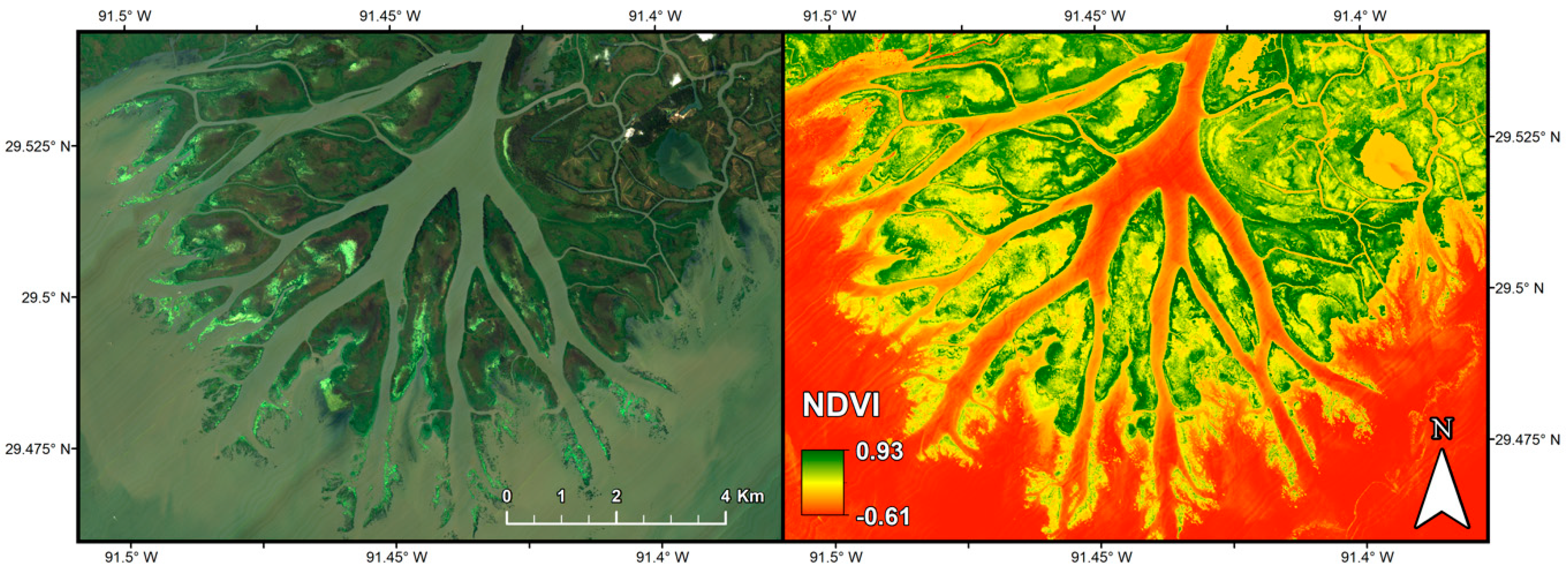
| Acquisition Dates | 17 October 2016 (Mosaic, Figure 2); 6–9 May 2015; 2–6 June 2015 | 17 October 2016 (Mosaic, Figure 3); 9 May 2015 |
| Aircraft Platform | B200 King Air | Gulfstream-III |
| Wavelength/Frequency | 380–2510 nm (Passive Radiance Measurements) | Fully polarimetric L-band; 0.2379 m/1.26 GHz (Transmitted Frequency) |
| Spectral Resolution | 5 nm ± 0.5 nm | 80 MHz (Chirp Bandwidth) |
| Spatial Resolution | 5.4 m | 5 m |
| Direct Model Inputs | Reflectance | Horizontally-Transmitted, Vertically-Received Backscatter |
| Derived Model Inputs | NDVI; First-Derivative of Reflectance | Volume and Double Bounce Scattering Components |
| Classification Data | Reference Data | |||
|---|---|---|---|---|
| Forested Wetland | Herbaceous Wetland | Other Vegetation | All | |
| Forested wetland | 21 | 0 | 0 | 21 |
| Herbaceous wetland | 1 | 67 | 0 | 68 |
| Other vegetation | 0 | 6 | 48 | 54 |
| All | 22 | 73 | 48 | 143 |
| User’s Accuracy (%) | Producer’s Accuracy (%) | |
|---|---|---|
| Forested wetland | 100.00 | 95.45 |
| Herbaceous wetland | 98.53 | 91.78 |
| Other vegetation | 88.89 | 100.00 |
| Overall accuracy | 95.10 | |
| Kappa | 0.92 | |
| Herbaceous AGB Models (n = 25, mean = 359.24 g/m2) | Forest AGB Models (n = 36, mean = 25,555 g/m2) | |||||||||||
|---|---|---|---|---|---|---|---|---|---|---|---|---|
| PLS Comps | R2 | RMSE | MAE | AIC | p | PLS Comps | R2 | RMSE | MAE | AIC | p | |
| 1. NDVI | 0.08 | 150.59 | 111.38 | 325.68 | 0.18 | 0.08 | 16,309 | 13,033 | 805 | 0.11 | ||
| 2. Reflectance PLSR | 3 | 0.33 | 180.51 | 92.21 | 4 | 0.45 | 20,418 | 9974 | ||||
| 3. First Derivative PLSR | 2 | 0.46 | 189.62 | 81.65 | 2 | 0.35 | 19,708 | 11,260 | ||||
| 4. HV Backscatter | 0.01 | 156.06 | 108.04 | 327.46 | 0.65 | 0.01 | 16,874 | 14,248 | 803 | 0.05 | ||
| 5. Volume, Double Bounce Components | 0.08 | 150.58 | 100.85 | 327.67 | 0.41 | 0.35 | 13,706 | 11,409 | 794 | <0.01 | ||
| 6. NDVI, HV Backscatter | 0.08 | 150.42 | 110.79 | 327.62 | 0.40 | 0.09 | 16,138 | 13,007 | 806 | 0.19 | ||
| 7. NDVI, Volume, Double Bounce | 0.23 | 137.22 | 99.91 | 325.03 | 0.13 | 0.38 | 13,375 | 10,972 | 794 | <0.01 | ||
| 8. Reflectance PLS X-Scores, HV Backscatter | 3 | 0.41 | 120.25 | 89.51 | 320.43 | 0.03 | 4 | 0.45 | 12,583 | 9979 | 794 | <0.01 |
| 9. Derivative PLS X-Scores, HV Backscatter | 2 | 0.51 | 109.24 * | 79.44 | 313.63 * | <0.01 | 2 | 0.36 | 13,560 | 11,311 | 795 | <0.01 |
| 10. Reflectance PLS X-Scores, Volume, Double | 3 | 0.42 | 117.73 | 86.99 | 322.21 | 0.05 | 4 | 0.53 * | 11,626 * | 8489 * | 790 * | <0.01 |
| 11. Derivative PLS X-Scores, Volume, Double Bounce | 2 | 0.51 * | 110.10 | 77.07 * | 316.02 | <0.01 | 2 | 0.48 | 12,233 | 10,066 | 790 * | <0.01 |
| Herbaceous MAE (g/m2) | Forest MAE (g/m2) | |
|---|---|---|
| 2. Reflectance PLSR | 112.57 | 12,061 |
| 3. First derivative PLSR | 110.05 | 14,192 |
| 4. HV backscatter | 114.71 | 16,481 |
| 5. Volume, double bounce components | 111.71 | 12,477 |
| 7. NDVI, volume, double bounce components | 118.35 | 12,040 |
| 8. Reflectance PLS X-scores, HV backscatter | 114.67 | 12,346 |
| 9. Derivative PLS X-scores, HV backscatter | 110.47 | 14,345 |
| 10. Reflectance PLS X-scores, volume, double bounce | 114.43 | 11,060 * |
| 11. Derivative PLS X-scores, volume, double bounce | 106.38 * | 12,950 |
© 2019 by the authors. Licensee MDPI, Basel, Switzerland. This article is an open access article distributed under the terms and conditions of the Creative Commons Attribution (CC BY) license (http://creativecommons.org/licenses/by/4.0/).
Share and Cite
Jensen, D.; Cavanaugh, K.C.; Simard, M.; Okin, G.S.; Castañeda-Moya, E.; McCall, A.; Twilley, R.R. Integrating Imaging Spectrometer and Synthetic Aperture Radar Data for Estimating Wetland Vegetation Aboveground Biomass in Coastal Louisiana. Remote Sens. 2019, 11, 2533. https://doi.org/10.3390/rs11212533
Jensen D, Cavanaugh KC, Simard M, Okin GS, Castañeda-Moya E, McCall A, Twilley RR. Integrating Imaging Spectrometer and Synthetic Aperture Radar Data for Estimating Wetland Vegetation Aboveground Biomass in Coastal Louisiana. Remote Sensing. 2019; 11(21):2533. https://doi.org/10.3390/rs11212533
Chicago/Turabian StyleJensen, Daniel, Kyle C. Cavanaugh, Marc Simard, Gregory S. Okin, Edward Castañeda-Moya, Annabeth McCall, and Robert R. Twilley. 2019. "Integrating Imaging Spectrometer and Synthetic Aperture Radar Data for Estimating Wetland Vegetation Aboveground Biomass in Coastal Louisiana" Remote Sensing 11, no. 21: 2533. https://doi.org/10.3390/rs11212533
APA StyleJensen, D., Cavanaugh, K. C., Simard, M., Okin, G. S., Castañeda-Moya, E., McCall, A., & Twilley, R. R. (2019). Integrating Imaging Spectrometer and Synthetic Aperture Radar Data for Estimating Wetland Vegetation Aboveground Biomass in Coastal Louisiana. Remote Sensing, 11(21), 2533. https://doi.org/10.3390/rs11212533