Joint Retrieval of Growing Season Corn Canopy LAI and Leaf Chlorophyll Content by Fusing Sentinel-2 and MODIS Images

Abstract

Continuous and accurate estimates of crop canopy leaf area index (LAI) and chlorophyll content are of great importance for crop growth monitoring. These estimates can be useful for precision agricultural management and agricultural planning. Our objectives were to investigate the joint retrieval of corn canopy LAI and chlorophyll content using filtered reflectances from Sentinel-2 and MODIS data acquired during the corn growing season, which, being generally hot and rainy, results in few cloud-free Sentinel-2 images. In addition, the retrieved time series of LAI and chlorophyll content results were used to monitor the corn growth behavior in the study area. Our results showed that: (1) the joint retrieval of LAI and chlorophyll content using the proposed joint probability distribution method improved the estimation accuracy of both corn canopy LAI and chlorophyll content. Corn canopy LAI and chlorophyll content were retrieved jointly and accurately using the PROSAIL model with fused Kalman filtered (KF) reflectance images. The relation between retrieved and field measured LAI and chlorophyll content of four corn-growing stages had a coefficient of determination (R²) of about 0.6, and root mean square errors (RMSEs) ranges of mainly 0.1–0.2 and 0.0–0.3, respectively. (2) Kalman filtering is a good way to produce continuous high-resolution reflectance images by synthesizing Sentinel-2 and MODIS reflectances. The correlation between fused KF and Sentinel-2 reflectances had an R² value of 0.98 and RMSE of 0.0133, and the correlation between KF and field-measured reflectances had an R² value of 0.8598 and RMSE of 0.0404. (3) The derived continuous KF reflectances captured the crop behavior well. Our analysis showed that the LAI increased from day of year (DOY) 181 (trefoil stage) to DOY 236 (filling stage), and then increased continuously until harvest, while the chlorophyll content first also increased from DOY 181 to DOY 236, and then remained stable until harvest. These results revealed that the jointly retrieved continuous LAI and chlorophyll content could be used to monitor corn growth conditions.

1. Introduction

Corn (Zea mays) is planted widely around the world, and is vital for food security both as food and fodder. Therefore, corn growth monitoring and yield prediction are very important for food security and sustainable development. Compared with yield prediction, crop growth monitoring can reveal problems such as nutrient deficiencies, water stress, or pest infestations in a timely way during the growing season [1]. Furthermore, information about crop growth is vital for monitoring crop behavior and predicting crop yield.

Remotely sensed spectral reflectances have already been shown to provide precise and timely information of corn plants status [2,3]. Available satellite images discriminate corn growth conditions by exploiting the spectral characteristic of reflected solar radiation. Leaf area index (LAI), defined as one-half of the total intercepting leaf area per unit, and the projected horizontal ground surface area for non-flat plant canopies [4,5,6], affects the photosynthesis of corn plants and carbon storage for light capture. Chlorophylls Chl a and Chl b are essential pigments for the conversion of light energy [7]. Remote sensing reflectance from the corn canopy is affected by corn canopy LAI and chlorophyll content [8,9,10,11], which gives an indirect estimate of nutrient status, plant stress, and productivity [12]. Therefore, both the LAI and chlorophyll content of corn are retrieved using the reflectance of remote sensing images in this study.

Corn growth monitoring is often hampered by the lack of high temporal and high spatial resolutions satellite time series [13]. One reason is that the corn is growing in the hot rainy season. Consequently, there are usually only few cloud-free spectral images available for the entire corn-growing season. Another reason is that high spatial resolution satellite images generally have a coarse temporal resolution [14]. Then, there are few images with both high spatial and temporal resolution during the corn-growing season. One promising solution for producing high spatial and temporal resolution images is fusing multi-source remote sensing images that may have different spatial and temporal resolutions. Existing image spatiotemporal fusion models can be classified into five major categories: (i) empirical; (ii) semi-empirical; (iii) spatial unmixing; (iv) machine learning; and (v) data assimilation [15,16].

The Spatial and Temporal Adaptive Reflectance Fusion Model (STARFM) [17], the Enhanced STARFM (ESTARFM) [18,19], the Non-Local Linear Regression (NL-LR) model [20] are all empirical fusion methods. The STARFM method can use the correlation among multi-source images to blend and minimize the system biases between different images acquired at the same time [18]. However, STARFM can’t handle the directional dependence of image reflectances, so Roy et al. developed a semi-physical fusion method to overcome this limitation [21]. The spatial unmixing method is more precise and derives fine spatial resolution information from interpreted fine spatial resolution satellite or aerial images or land-use databases [22]. Its limitation lies in requiring approximately simultaneous high spatial resolution images or thematic maps from a different source. Learning-based fusion methods provide a promising approach for predicting both phenological and type changes [16,23]. Compared to the aforementioned methods, data-assimilation methods can optimally combine observation information and their respective uncertainties to minimize the residual errors [24,25]. Huang et al. fused Landsat Thematic Mapper (TM) LAI images derived empirically from the soil-adjusted vegetation index (SAVI) and normalized difference vegetation index (NDVI) with the four-day composite, 1-km spatial resolution, Moderate Resolution Imaging Spectroradiometer (MODIS) LAI product (MCD15A3) [15]. These vegetation indexes were produced by combining the red band and near-infrared (NIR) band for revealing the crop growth and change. Compared with an empirical estimation of LAI and chlorophyll content, which is based on the statistical regression with image spectral reflectance or vegetation indices (VIs) [26,27], physical process-based methods do not need a large amount of measured data, and aren’t affected by crop cultivars, growth stage, and environmental conditions once the model inputs are determined [28]. The PROSAIL model is a popular physical radiative transfer model for crop canopy LAI and chlorophyll content retrieval [29]. PROSAIL was developed by coupling the canopy-scale SAIL bidirectional canopy-reflectance model [30] with the leaf-scale PROSPECT model [31,32] in the 1990s. Many researchers have estimated canopy biophysical variables using the PROSAIL model for agricultural applications [33,34]. Botha et al. retrieved potato canopy leaf chlorophyll from a hyperspectral image using the PROSAIL model [35]. Darvishzadeh et al. retrieved rice canopy chlorophyll content using a lookup-table (LUT) [36]. Rivera et al. also improved the retrieval of leaf chlorophyll content and LAI using the PROSAIL model with multiple cost functions and regularization options [37]. Duan et al. [38] retrieved the LAI of maize, potato, and sunflower using the PROSAIL model from unmanned aerial vehicle (UAV) hyperspectral images. Li et al. retrieved winter wheat canopy LAI and leaf chlorophyll content using the PROSAIL model by including prior agronomic knowledge [33]. In general, crop canopy LAI and chlorophyll content are correlated, and a closed corn canopy is never associated with low chlorophyll content (Baret, 2016). However, the aforementioned researches didn’t consider exploiting the correlation between crop canopy LAI and leaf chlorophyll content when retrieving these two parameters simultaneously. In this paper, we investigated the joint retrieval of corn canopy LAI and chlorophyll content using fused high spectral and spatial resolution images and taking into account the interactions of LAI with chlorophyll content.

The specific objective of this study was to develop a framework for retrieving the corn canopy LAI and chlorophyll content jointly for continuous corn growth monitoring using the fused high spatial and temporal resolution images from Sentinel-2 image and MODIS images. Our overarching aim was to answer the following questions:

• Can the Kalman filter be used to fuse Sentinel-2 and MODIS reflectances for producing higher spatial and temporal resolutions images?
• Can the corn canopy LAI and chlorophyll content be retrieved jointly and accurately during the entire corn growing season? Which growing stages are retrieved better?
• Can the retrieved time series of LAI and chlorophyll content be used to monitor the corn growing behavior and how?

2. Materials and Pre-Processing

2.1. Study Area

The study area spans three counties (Zhuozhou, Gaobeidian, and Dingxing) of Baoding City, Hebei Province, China, ranging from 115°29′, 39°5′ to 116°14′E, 39°35′N (Figure 1), which is the main corn-planting area in northern China. The region has a temperate continental monsoon climate with an annual average rainfall of 550 mm and an annual sunshine rate of about 60%. The corn-growing season temperature ranges from 7 °C to 39 °C. The soil is fertile, and the summer is hot and rainy. The fields are cultivated in a rotation with corn and winter wheat (Triticum aestivum), and soybean (Glycine max), cotton (Gossypium hirsutum), and sweet potato (Ipomoea batatas) are grown occasionally. Corn is generally sown at the beginning of June and harvested at the beginning of September, with a three-month growing period. Usually, corn is in the seedling stage in mid-June, the seven-leaf stage at the end of June, the jointing stage in early July, the anthesis-silking stage in the middle of August, the milking stage at the end of August, and the mature period in the middle of September.

All the corn fields in study area were managed well for irrigation and fertilization by local farmers, and all the corn plants were healthy without disease/insect attacks and drought. There were 12 in situ measured sites (Figure 1b) in the study area totally, and there were four to five samplings illustrated as Figure 1c in each site. These in situ measured data were used for validating the Kalman filtered (KF) reflectance, setting up the co-distribution between LAI and chlorophyll content, and validating the retrieving accuracy of LAI and chlorophyll content.

2.2. Field Data Collection

Field data were collected four times in 2017 for the assessment of the accuracy of the joint retrieval on the dates shown in Figure 2 and labeled as “ ”. The parameters collected included LAI, chlorophyll content of corn leaves, and spectra of corn canopy, corn leaves, and soil. There were 61 in-situ measured samplings distributed in these three counties of Zhouzhou, Gaobeidian and Dingxing randomly and evenly. All the samplings were geolocated using a Huace i80 real-time kinematic (RTK) GPS receiver (Huace Ltd., Shanghai, China). Corn canopy LAI was measured using an LAI-2200 Plant Canopy Analyzer (LI-COR, Lincoln, NE, USA) with a 45° field angle to eliminate the effect of non-plant objects within the range of the sensor’s field of view. For each in situ LAI measurement, two repeats were done including one above canopy and four below canopy readings [39].

In addition, leaf chlorophyll content was measured using an SPAD-502 leaf chlorophyll meter (Konica Minolta Corp., Solna, Sweden) nondestructively. The SPAD readings were unitless, which were highly correlated with foliage chlorophyll content (μg/cm²). The empirical calibration function developed by Darvishzadeh et al. [40] and Markwell et al. [41] was used to convert our SPAD readings to foliage chlorophyll content (μg/cm²) in this study. Five corn plants were selected randomly in each plot, and six leaves per plant were used to measure the chlorophyll content. For each corn plant, chlorophyll content was measured in the leaf tip, bottom, and middle. The average of these measurements was used to represent the chlorophyll content for each leaf, and the average for all leaves was used to represent the chlorophyll content in each plot.

The spectra of corn canopy, corn leaves, and soil were measured using an SVC HR-1024 spectrometer (Spectra Vista Corporation, Poughkeepsie, NY, USA). Each sample was measured five times and averaged to represent the spectra.

2.3. Remote Sensing Images and Pre-Processing

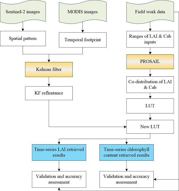
Thirteen cloud-free MODIS images at 250-m spatial resolution were acquired from the Terra Surface Reflectance product (MOD09GA) between 27 June (day of year, or DOY 178) and 23 September (DOY 266), 2017 (see Figure 2 for the dates), covering the field-measured dates of the seventh leaf stage (DOY 193, 12 July), jointing stage (DOY 211, 30 July), filling stage (DOY 236, 24 August), and milking stage (DOY 242, 30 August). In contrast, only five cloud-free Sentinel-2 images were available. All the MODIS imagery is made available free of charge by National Aeronautics and Space Administration (NASA) (http://reverb.echo.nasa.gov/reverb), while Sentinel-2 imagery is made available free of charge by European Space Agency (ESA) (https://scihub.copernicus.eu/dhus/#/home).

The time-series of the MOD09GA images was pre-processed using the MODIS Reprojection Tool (MRT), and georeferenced to the UTM projection and WGS84 coordinate system with 250-m spatial resolution. The parameter settings were saved in the *.prm file, and batch pre-processing was conducted using this *.prm file. In a similar fashion, the five Sentinel-2 images were georeferenced to the same coordinate system using 21 field-measured ground control points. After geometric correction, the root mean square error (RMSE) of the calculated and measured locations was less than one pixel (10 m) for each Sentinel-2 image. Atmospheric correction was performed using the Sentinel Application Platform SNAP [42] to obtain the reflectance in each band [43].

3. Methods

Our joint retrieval of growing season corn canopy LAI and chlorophyll content involved two steps: one was fusing Sentinel-2 and MODIS images to generate an improved time series of synthetic images using the Kalman filter algorithm, and the other was the joint retrieval of corn canopy LAI and chlorophyll content for the growing season from the generated time series of synthetic images. The generated time series of synthetic reflectances was matched with the reflectances in the LUT, and the weighted cost function was used to decide the optimal matching. LAI and chlorophyll content were retrieved jointly during this matching process. The workflow for fusing two kinds images and joint retrieval for LAI and chlorophyll content is as shown in Figure 3.

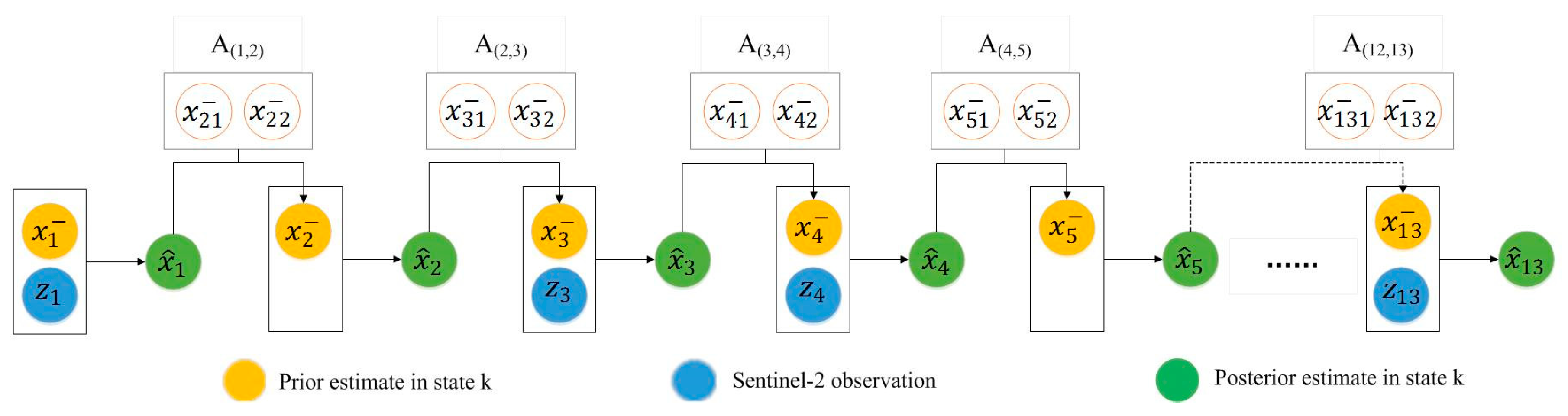
3.1. Fusing Sentinel-2 and MODIS Images for Time Series Synthetic Images

The Kalman filter recursive algorithm [44] was used to fuse Sentinel-2 and MODIS images to generate a time series of synthetic reflectances with higher temporal and spatial resolution. Sedano et al. [25] and Huang et al. [15] fused Landsat TM images (30-m spatial resolution) and MODIS images (250-m spatial resolution) for generating a time series of synthetic NDVI/LAI values with a medium spatial resolution (30 m) at four-day intervals. In this study, we fused Sentinel-2 images (spatial resolution of 10 m) and MODIS images (spatial resolution of 250 m) to explore if this kind of spatial resolution difference (i.e., 250 m/10 m) could be fused with a higher accuracy. There are two submodels, including the state update model and measurement update model, which characterize the temporal dynamics and capture the relationship between two kinds of reflectance pixel values, respectively. These two updates are calculated as follows:

$$x_k=A{x}_{k-1}+w_{k-1},$$

(1)

$$z_k=H{x}_k+v_k,$$

(2)

where $x_k$ and $x_{k-1}$ are the estimated values for the present state k and previous state k−1, respectively. For image fusing in this study, $x_k$ and $x_{k-1}$ are the MODIS reflectances at time k and k−1, respectively (Figure 4). The connection between time k and k−1 is done by the state-transition matrix A, and the observed value $z_k$ is linearly related to the current state estimation $x_k$. In addition, H is a measurement sensitivity matrix. The variables $w_{k-1}, v_k$ are process noise and measurement noise, respectively. The time update is as follows:

$${\widehat{x}}_k^{-}=a\ast {\widehat{x}}_{k-1}+b,$$

(3)

$$P_k^{-}=A{P}_{k-1}^{-}{A}^T+w_{k-1},$$

(4)

where ${\widehat{x}}_k^{-}$ is the prior estimate of the present (k) state; ${\widehat{x}}_{k-1}$ is the posterior estimate of the variable in the previous (k-1) state; $P_k^{-}$ is the prior uncertainty at the present (k) state; and $P_{k-1}^{-}$ is the prior uncertainty in the previous (k-1) state. T represents the matrix transposition operation. During the observation updating, the prior estimates (Equation (5)) and their uncertainties (Equation (6)) are updated with new observations. ${\overline{K}}_k$ is Kalman gain, which effectively weights the prior state and the measurements by their respective uncertainties. $P_k$ is the uncertainties of the previous state and the present observation [15,25,45].

$${\widehat{x}}_k=x_k^{-}+{\overline{K}}_k\left[z_k-H_k{x}_k^{-}\right],$$

(5)

$${\overline{K}}_k=P_k^{-}{H}_k{}^T{\left[H_k{P}_k^{-}{H}_k{}^T+R_k\right]}^{-1},$$

(6)

$$P_k=\left(1-{\overline{K}}_k{H}_k\right)P_k^{-},$$

(7)

Figure 4 illustrates the scheme of the KF approach for fusing Sentinel-2 and time-series MODIS images. During the fusing process, the available Sentinel-2 images were used as observations, and the time-series MODIS images were used for capturing the phenological trajectories of corn canopy reflectance over time.

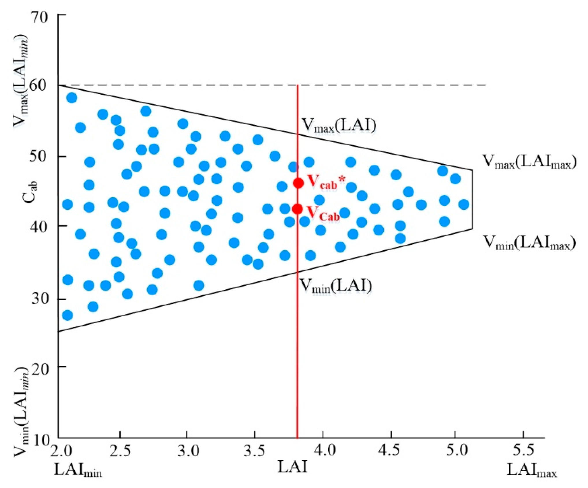
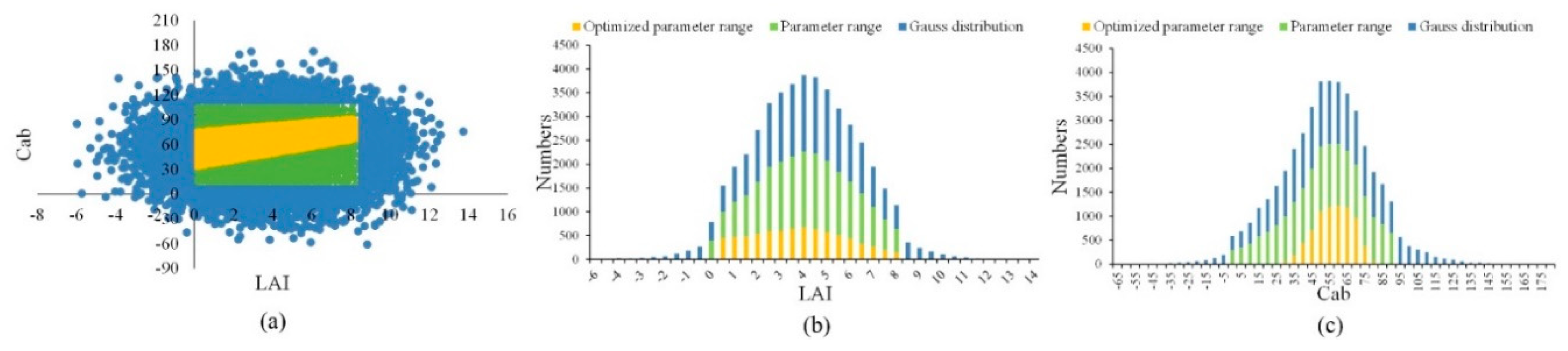
3.2. Joint Retrieval of Growing Season Corn Canopy LAI and Chlorophyll Content

The relationship between corn canopy LAI and chlorophyll content was exploited for the joint retrieval of two variables in this study. Some researchers observed that a closed corn canopy was never related to low chlorophyll content [46,47]. Therefore, we proposed to set up the co-contributions by restricting the chlorophyll content range as a function of the corn canopy LAI in different growing stages. Figure 5 shows the scheme of the co-distribution for corn canopy LAI and chlorophyll content in the filling stage. The maximum/minimum LAI values and the maximum/minimum chlorophyll content values were determined by field-measured data where 15,000 random numbers were generated using the range of LAI and chlorophyll content listed in

Table 1. Optimized inputs of PROSAIL for the different growing season stages of corn using the co-distributions.

Stage	$\mathit{L}\mathit{A}{\mathit{I}}_{\mathit{m}\mathit{i}\mathit{n}}$	$\mathit{C}\mathit{a}{\mathit{b}}_{\mathit{m}\mathit{i}\mathit{n}}(\mathit{L}\mathit{A}{\mathit{I}}_{\mathit{m}\mathit{i}\mathit{n}})$	$\mathit{C}\mathit{a}{\mathit{b}}_{\mathit{m}\mathit{a}\mathit{x}}(\mathit{L}\mathit{A}{\mathit{I}}_{\mathit{m}\mathit{i}\mathit{n}})$	$\mathit{L}\mathit{A}{\mathit{I}}_{\mathit{m}\mathit{a}\mathit{x}}$	$\mathit{C}\mathit{a}{\mathit{b}}_{\mathit{m}\mathit{i}\mathit{n}}(\mathit{L}\mathit{A}{\mathit{I}}_{\mathit{m}\mathit{a}\mathit{x}})$	$\mathit{C}\mathit{a}{\mathit{b}}_{\mathit{m}\mathit{a}\mathit{x}}(\mathit{L}\mathit{A}{\mathit{I}}_{\mathit{m}\mathit{a}\mathit{x}})$
1	0.100	30.249	54.100	3.590	42.623	59.919
2	0.570	34.039	63.823	5.851	47.358	70.469
3	1.621	32.227	65.973	6.491	48.557	73.932
4	1.991	40.212	69.956	6.580	52.002	75.979
5	1.341	44.960	69.690	6.111	56.924	75.728

Notes: Stage 1 is from 27 June to 12 July, Stage 2 is from 13 July to 3 August, Stage 3 is from 4 August to 15 August, Stage 4 is from 16 August to 1 September, and Stage 5 is from 2 September to 15 September in the study area.

. The maximum and minimum values of chlorophyll content corresponding to the given LAI values were used to set up the co-contributions by assuming they satisfy the Gaussian distribution. Furthermore, the co-contributions of corn canopy LAI and chlorophyll content were calculated with the formula in Equation (8) (Weiss and Baret, 2016). Theoretically, Equation (8) normalizes the LAI and chlorophyll content values. The left portion of the equation is the normalization of the chlorophyll content (V_Cab) corresponding to the minimum value of LAI, whereas the right portion is the normalization of a given chlorophyll content ($V_{Cab}{}^{\ast }$) with a given LAI value. The $V_{Cab}{}^{\ast }$ is the corn canopy chlorophyll content after linking its co-distribution to LAI. The values defining the co-distributions between corn canopy LAI and chlorophyll content are specified in Table 1. They were derived empirically based on the collected field data, assuming that large values of LAI correspond to a restricted range of chlorophyll content.

$$\frac{V_{Cab}-V_{\min \left({\mathrm{LAI}}_{min}\right)}}{V_{\max \left({\mathrm{LAI}}_{min}\right)}-V_{\min \left({\mathrm{LAI}}_{min}\right)}}=\frac{V_{Cab}{}^{\ast }-V_{\min \left(\mathrm{LAI}\right)}}{V_{\max \left(\mathrm{LAI}\right)}-V_{\min \left(\mathrm{LAI}\right)}},$$

(8)

The minimum and maximum values are defined as: $V_{min}\left(\mathrm{LAI}\right)=V_{min}\left({\mathrm{LAI}}_{min}\right)+\mathrm{LAI}\times \left(V_{min}\left(LA{I}_{max}\right)-V_{min}\left({\mathrm{LAI}}_{min}\right)\right)$ and $V_{max}\left(\mathrm{LAI}\right)=V_{max}\left({\mathrm{LAI}}_{min}\right)+\mathrm{LAI}\times \left(V_{max}\left(LA{I}_{max}\right)-V_{max}\left({\mathrm{LAI}}_{min}\right)\right)$.

Here, $V_{Cab}$ is the random value of chlorophyll content and $V_{Cab}{}^{\ast }$ is the random value of chlorophyll content that considers the joint probability distributions between corn canopy LAI and chlorophyll content. Through the co-distributions between corn canopy LAI and chlorophyll content, the small values of chlorophyll content corresponding to the largest LAI values were deleted, which can alleviate the ill-posed problem. The co-distribution provides a reasonable set of values for the joint retrieval of LAI and chlorophyll content, and optimizes the PROSAIL model inputs.

Using the co-distributions, the PROSAIL model inputs for the entire corn-growing season were optimized based on in situ measured corn canopy LAI and chlorophyll content. The optimized inputs are listed in Table 1. The LAI and chlorophyll content followed Gaussian distributions during this optimization process, which can be seen from Figure 6. Figure 6a is the scatter plot between LAI and chlorophyll content; Figure 6b,c are statistical retrievals of LAI and chlorophyll content with an optimized parameter range, parameter range, and mathematical Gaussian distribution. The blue areas correspond to the values with a Gaussian distribution, the green areas are the restricted values with the maximum and minimum values of measured LAI and chlorophyll content, and the yellow areas are the joint probability distributions of corn canopy LAI and chlorophyll content. We can see that the invalid, ambiguous values are removed step by step through each restriction operation.

After the restriction and optimization of the LAI and chlorophyll content values, the LUT was generated, and the cost function was used to find the best matching values between the simulated and observed reflectances in multiple bands. There are four kinds of inputs of the PROSAIL model for retrieving: leaf optical properties, canopy structure, background soil reflectance, and sun-view geometry [48]. Considering the sensitivity of PROSAIL inputs, the LAI and C_ab inputs were set using the former restriction conditions in Table 1 and Figure 5, and the other inputs were set in line with the setting in our previous work [48].

Cost functions using the RMSE between simulated and observed reflectances in multiple bands are often used for vegetation parameters retrieval [49,50]. A weighted RMSE was used in this study, which is expressed as follows:

$$D\left(P,Q\right)={\sum }_{{\lambda }_i=1}^{{\lambda }_n}{w}_i{\left(p\left({\lambda }_i\right)-q\left({\lambda }_i\right)\right)}^2,$$

(9)

where $D\left(P,Q\right)$ is the cost function, ${\lambda }_i$ is the ith bands, $p\left({\lambda }_i\right)$ is the reflectance in band ${\lambda }_i$, $q\left({\lambda }_i\right)$ is the simulated reflectance in band ${\lambda }_i$, n is the number of bands, and $w_i$ is the weight of band ${\lambda }_i$, which is the reciprocal of the reflectance in band ${\lambda }_i$. The retrieved LAI and chlorophyll content are found by minimizing the RMSE.

4. Results and Analysis

4.1. Spatial Distribution of the Synthetic KF Reflectance

Figure 7 shows a subset of the reflectance images in four bands (blue, green, red, and near infrared (NIR)) at DOY 193 for MODIS, Sentinel-2, synthetic KF images, and the scatter plots of the Sentinel-2 and the KF reflectances. The spatial variations in both MODIS and Sentinel-2 reflectances had the same structure as the KF reflectance. The subset image included areas of cropland, roads, river, forest, and buildings. The boundaries between land objects and the spatial structure can be clearly identified in both Sentinel-2 and KF images. The spatial variations of the MODIS images are similar to those of the Sentinel-2 and KF images; however, the details in the MODIS images are unclear because of their coarse spatial resolution. In order to assess the similarity between the KF and Sentinel-2 images, we analyzed the scatter plots between the Sentinel-2 and the KF reflectances. Figure 7d,h,l,p display the scatter plots between the Sentinel-2 and KF reflectances in the blue, green, red, and NIR, respectively, showing that, aside from a small deviation, they are close to the 1:1 line for the three visible bands. A similar trend can also be seen for the NIR band, except that there is a bias on the Y-axis, which indicates that the Sentinel-2 reflectance is systematically higher than the KF reflectance. This deviation occurs because the KF reflectance is the compromise between Sentinel-2 reflectance and MODIS reflectance, and the MODIS pixels were mostly all mixed pixels.

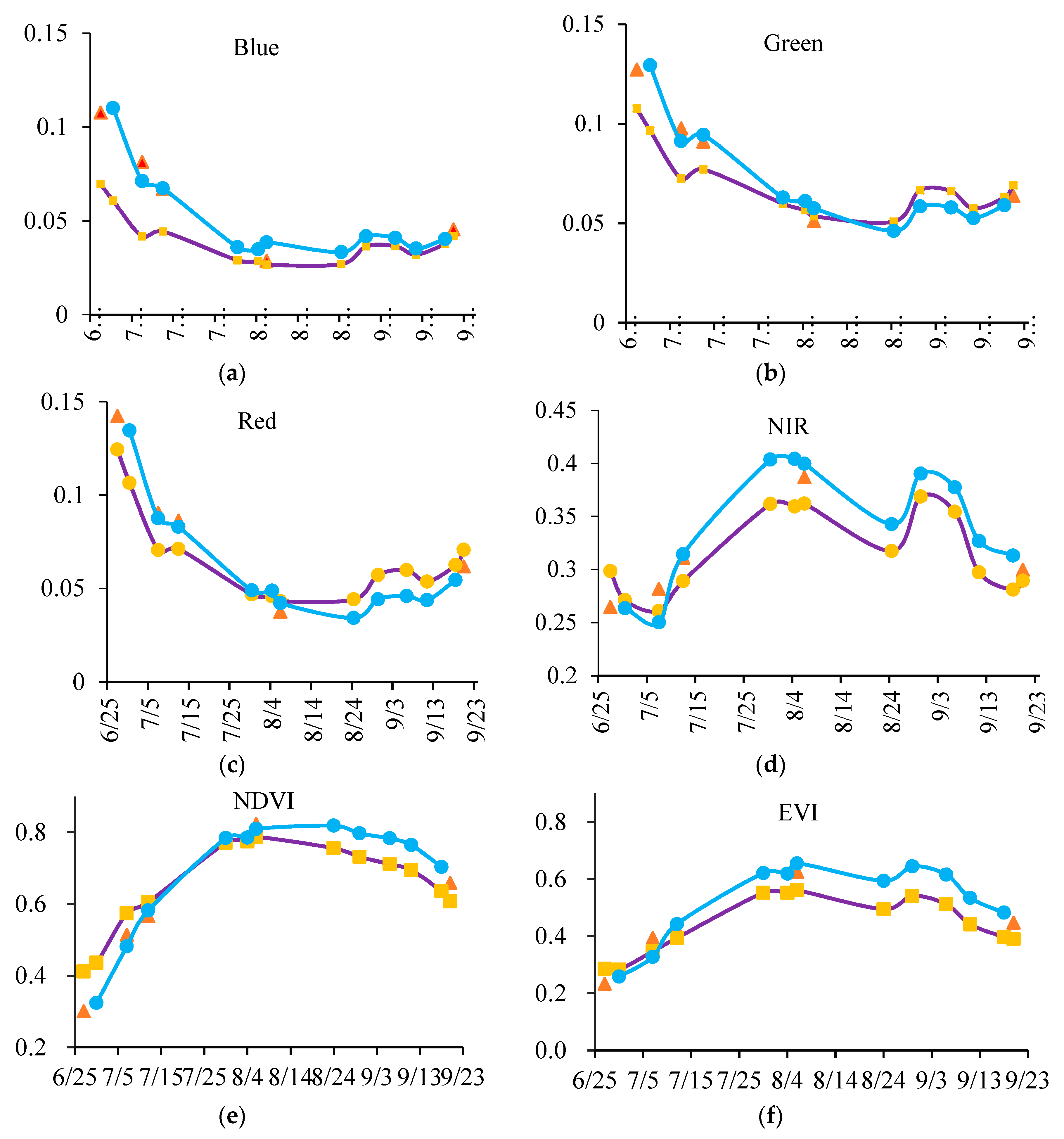
4.2. Time Series of Synthetic KF Reflectance and NDVI, EVI

The plots of the time series of the reflectance and vegetation indexes are shown in Figure 7, which were derived from the mean of the selected sampling of Figure 6. The five Sentinel-2 images were acquired on 7 July (DOY 188), 12 July (DOY 193), and 6 August (DOY 218), respectively. Figure 8a–c show downward trends from 25 June (DOY 177) to 24 August (DOY 236) in the blue, green, and red bands, besides the slightly rising or unchanging from 7 July (DOY 188) to 12 July (DOY 193). Comparatively speaking, there was no distinct regularity for the changing on the NIR band, and there were two fluctuations from 25 June (DOY 177) to 24 August (DOY 236), respectively. Moreover, the time-series vegetation indexes including NDVI (Figure 8e) and EVI (Figure 8f) were used to characterize corn-growing change. In comparison to the NDVI plot, there was a big fluctuation in the EVI from 4 August (DOY 216) to 30 August (DOY 242). For both vegetation indexes, the KF images were similar to the Sentinel-2 ones; the MODIS EVI was lower than the Sentinel-2 EVI and the fused KF EVI during the entire growing season, while the MODIS NDVI was higher than the Sentinel-2 NDVI and fused KF NDVI before 30 July (DOY 211), and lower from 30 July (DOY 211) to 20 September (DOY 263). Generally speaking, the Kalman-filtered image reflectances agree better with Sentinel-2 reflectances than MODIS reflectances for all four spectral bands and two vegetation indexes.

In addition, Figure 8 shows that the KF reflectances approach the Sentinel-2 reflectances, and the changing footprint of the time-series KF reflectances was similar to the changing of MODIS reflectances. This result is ascribed to the principle of Kalman filter that the spatial specifics of KF images originate from Sentinel-2 images, and the temporal changes originate from MODIS images.

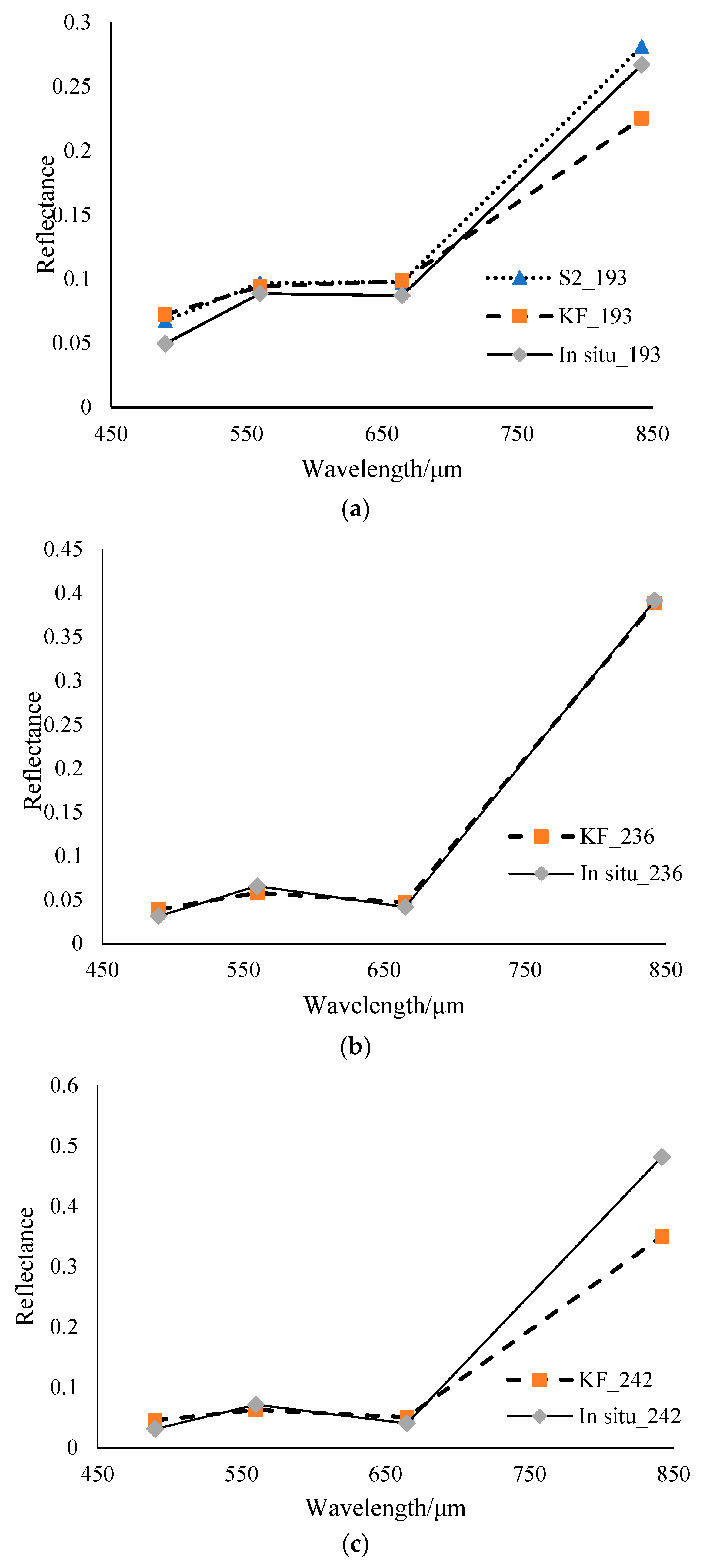
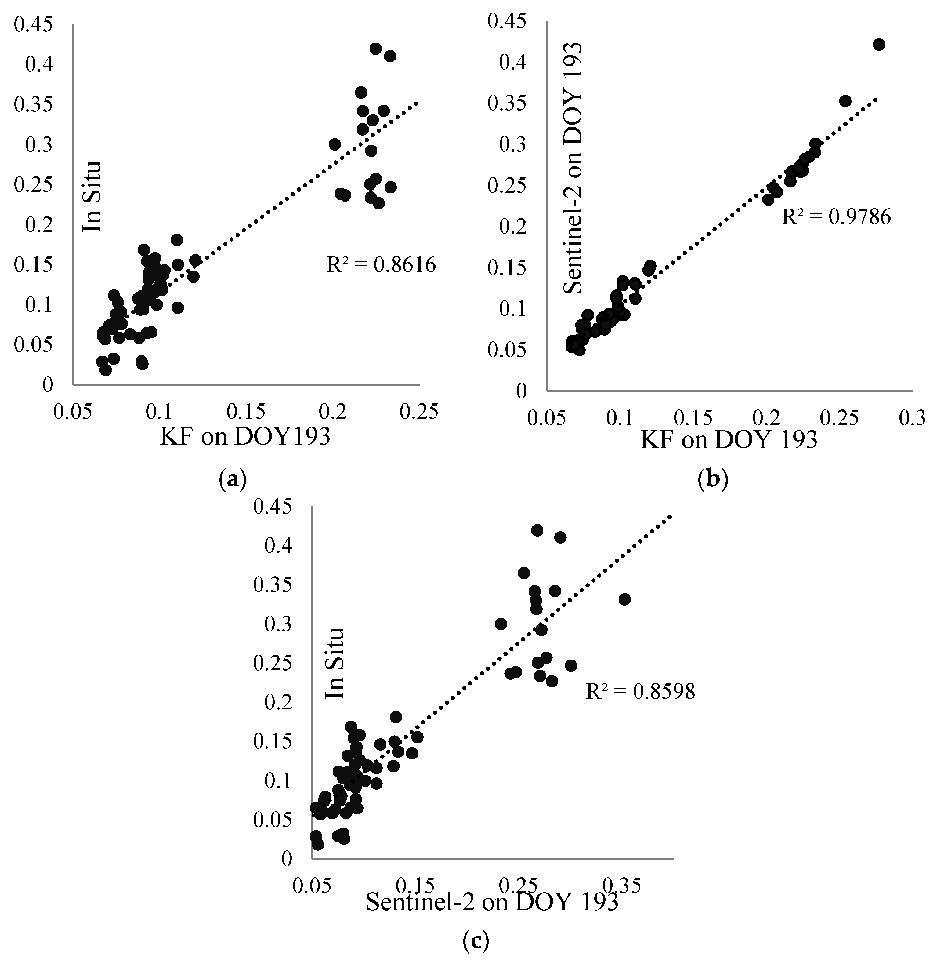
4.3. Accuracy Assessment of Synthetic KF Reflectance using Field-Measured Reflectance

The accuracy of the synthetic KF reflectances was assessed using the field-measured reflectances. Figure 9 shows the comparison of the synthetic KF and the measured reflectances within the blue, green, red, and NIR bands on DOY 193 (a), DOY 236 (b), and DOY 242 (c), respectively. The best accuracy is obtained for DOY 236, as shown in Figure 9b, when the synthetic KF reflectances were almost the same as the in situ measured reflectance in all bands. The synthetic KF reflectances were very close to the Sentinel-2 reflectances, and they were all higher than the measured reflectances in the blue, green, and red bands on DOY 193 (Figure 9a). However, the synthetic KF reflectances are lower than the Sentinel-2 reflectances and the measured reflectances on DOY 193 (Figure 9a). On DOY 242, neither Sentinel-2 nor MODIS data were available, so there were only the synthetic KF and the measured reflectances (Figure 9c). Similarly to the synthetic results of Figure 9a, the synthetic KF reflectance matched the measured reflectances in the blue, green, and red bands quite well, and was slightly higher than the measured reflectances for the NIR band on DOY 242 (Figure 9c).

To further assess the accuracy of the synthetic KF reflectance, we investigated the correlations between the KF reflectances with the Sentinel-2 and the field measured reflectance samplings on DOY 193. Figure 10a shows the scatter plots of the KF reflectance with the in situ measured reflectance with an R² value of 0.8616 and RMSE of 0.0401. Figure 10b shows that the coefficient of determination (R²) between the KF and the Sentinel-2 reflectances was 0.98 and the RMSE was 0.0133, which implies that the image details of the KF results were mainly contributed by the Sentinel-2 images. Figure 10c shows that the R² between Sentinel-2 and the in situ measured reflectance was 0.8598, and the RMSE was 0.0404.

4.4. Accuracy Assessment of Joint Retrieval of LAI and Chlorophyll Content Using Field-Measured Data

The RMSE, bias, and estimate accuracy (EA) were used to assess the accuracy of the joint retrieval of LAI and chlorophyll content.

Table 2. Accuracy assessment result of joint retrieval of corn canopy LAI and chlorophyll content.

	LAI						Cab (μg/cm2)
DOY	Correlation	R2	RMSE	Bias	EA (%)	SD	Correlation	R2	RMSE	Bias	EA (%)	SD
193	y = 1.74x − 1.66	0.62	0.30	0.60	63.90	0.21	y = 4.86x − 226.76	0.49	3.18	11.59	92.78	0.62
211	y = 0.74x + 1.04	0.53	0.30	0.36	90.56	0.42	y = 0.74x − 2.70	0.59	0.77	19.69	98.31	1.21
236	y = 0.76x + 0.81	0.62	0.36	0.38	91.67	0.60	y = 1.38x − 41.38	0.63	1.07	13.51	98.19	0.99
242	y = 0.65x + 1.41	0.60	0.30	0.29	92.55	0.56	y = 4.24x − 255.36	0.66	3.05	21.25	94.01	0.98

Notes: y is retrieved LAI or chlorophyll content (C_ab), x is the in situ measured LAI or chlorophyll content (C_ab).

shows the accuracy assessment results of the joint retrieval for corn canopy LAI and chlorophyll content. The R² had a p-value < 0.01 and 99.99% reliability for both the retrieved LAI and chlorophyll content. These results indicated that both the retrieved LAI and chlorophyll content were significantly correlated to the field-measured values.

RMSE is a measure of the differences between a model and a reference dataset. The RMSEs listed in Table 2 implied that the accuracy of retrieved LAI and chlorophyll content was high and with a low level of dispersion. The EA confirmed that the jointly retrieved LAI and chlorophyll content were accurate. More specifically, the retrieval accuracy of LAI and chlorophyll content on DOY 193 was lower than in the other three stages. Corn was in the seventh leaf stage on DOY 193, and the reflectance in the images included both corn canopy and soil. This resulted in the lower retrieval accuracy on DOY 193. EA is calculated as shown in Equation (10):

$$EA=\left(1-\frac{RMSE}{Mean}\right)\times 100\%,$$

(10)

4.5. Comparison of Retrieval of LAI and Chlorophyll Content Using Synthetic KF and Sentinel-2 Images

The relative error was used to assess the accuracy for retrieving LAI and chlorophyll content using the synthetic KF images and the Sentinel-2 images, respectively. Figure 11a shows that the relative error of LAI retrieval was mainly distributed in the range of 0.1–0.2 on DOY 188 and DOY 193. Instead, the relative error of LAI retrieval was mainly distributed in the range of 0.4–0.6 on DOY 218. It can be observed in Figure 7 that the error between the synthetic and the Sentinel-2 reflectances on DOY 218 was larger than on DOY 193, DOY 236, and DOY 242. This could be explained by a larger LAI retrieval error on DOY 218 than in the other days. Figure 11b shows that the relative error of chlorophyll content retrieval is mainly distributed in the range of 0.0–0.3 μg/cm² on DOY 188 and DOY 193. However, on DOY 218, the relative error of LAI retrieval was distributed across a larger range, from 0.3 to 1.2 μg/cm².

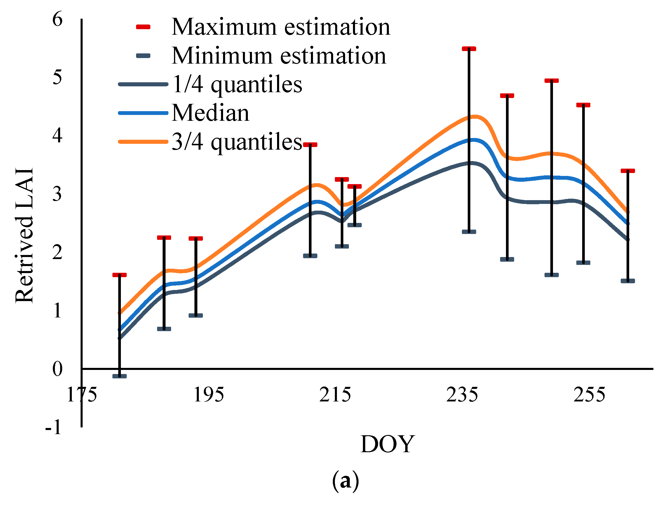
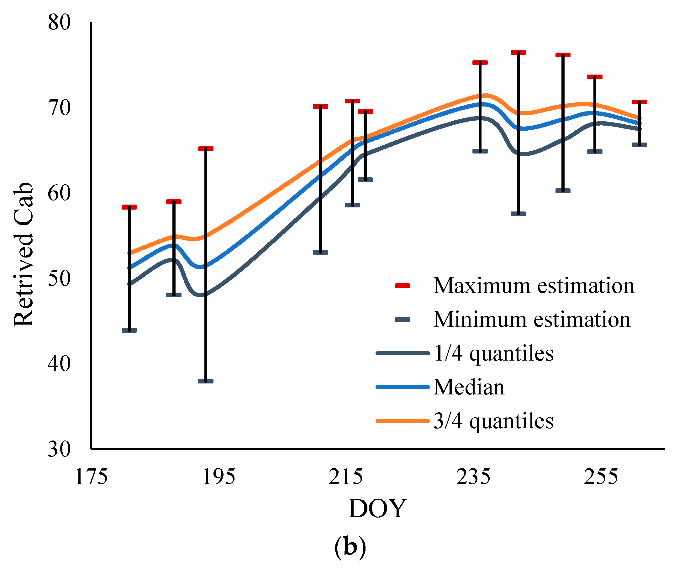
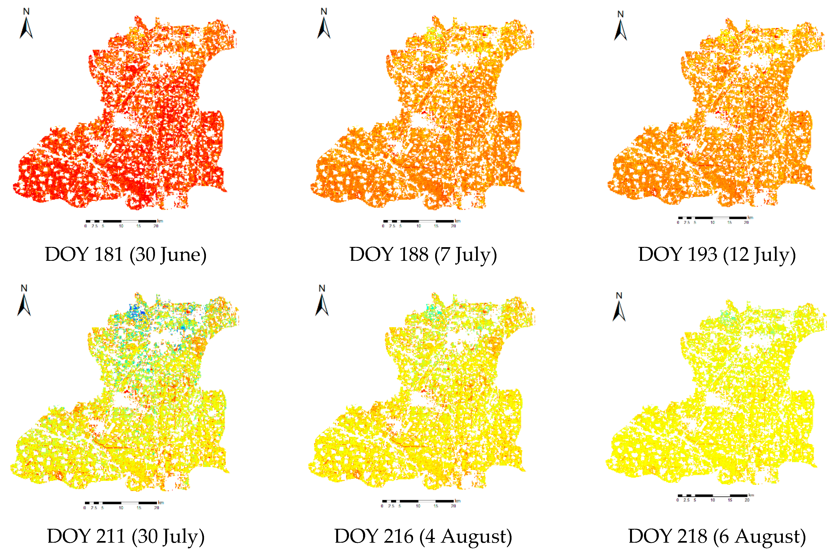
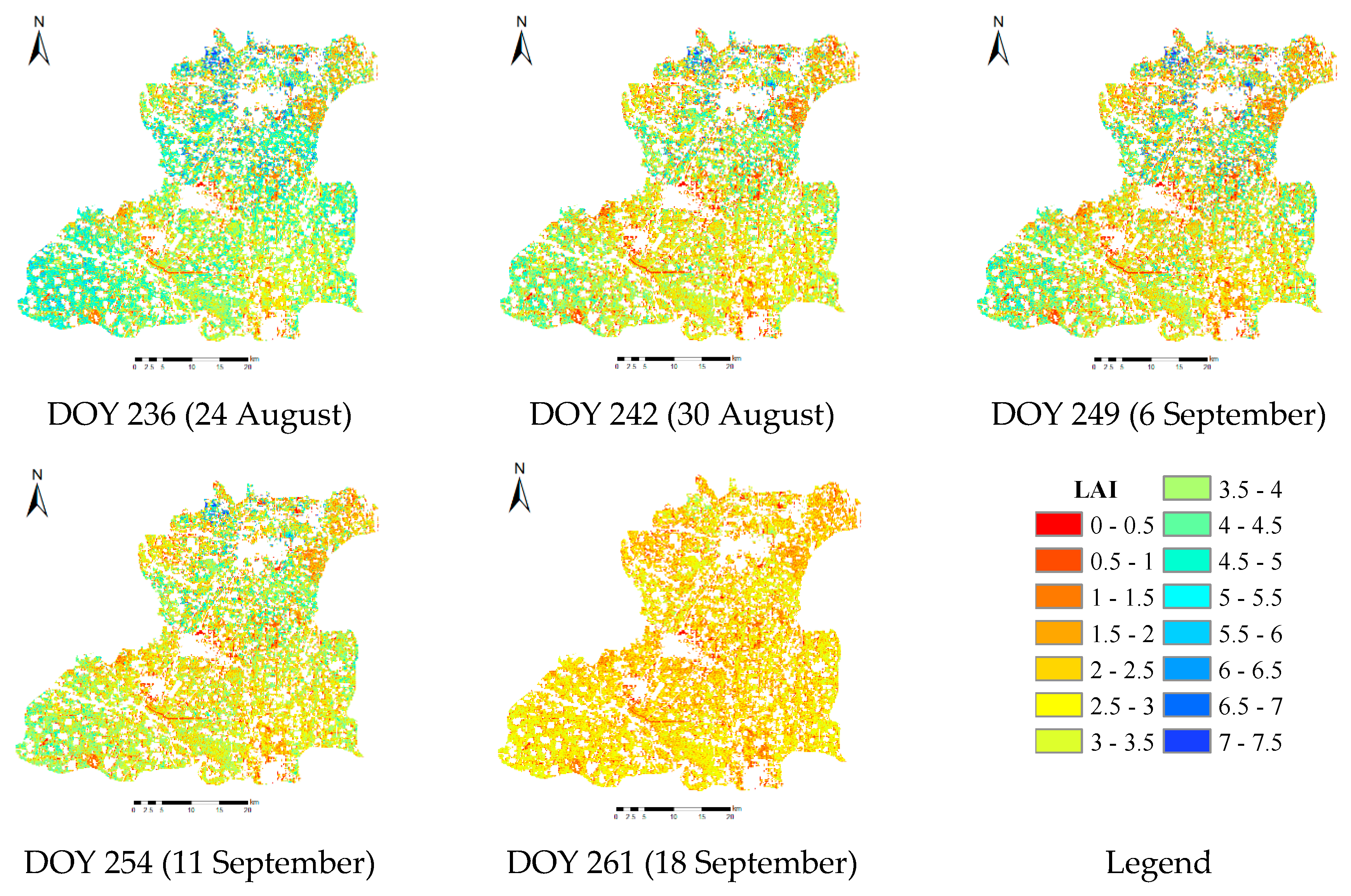
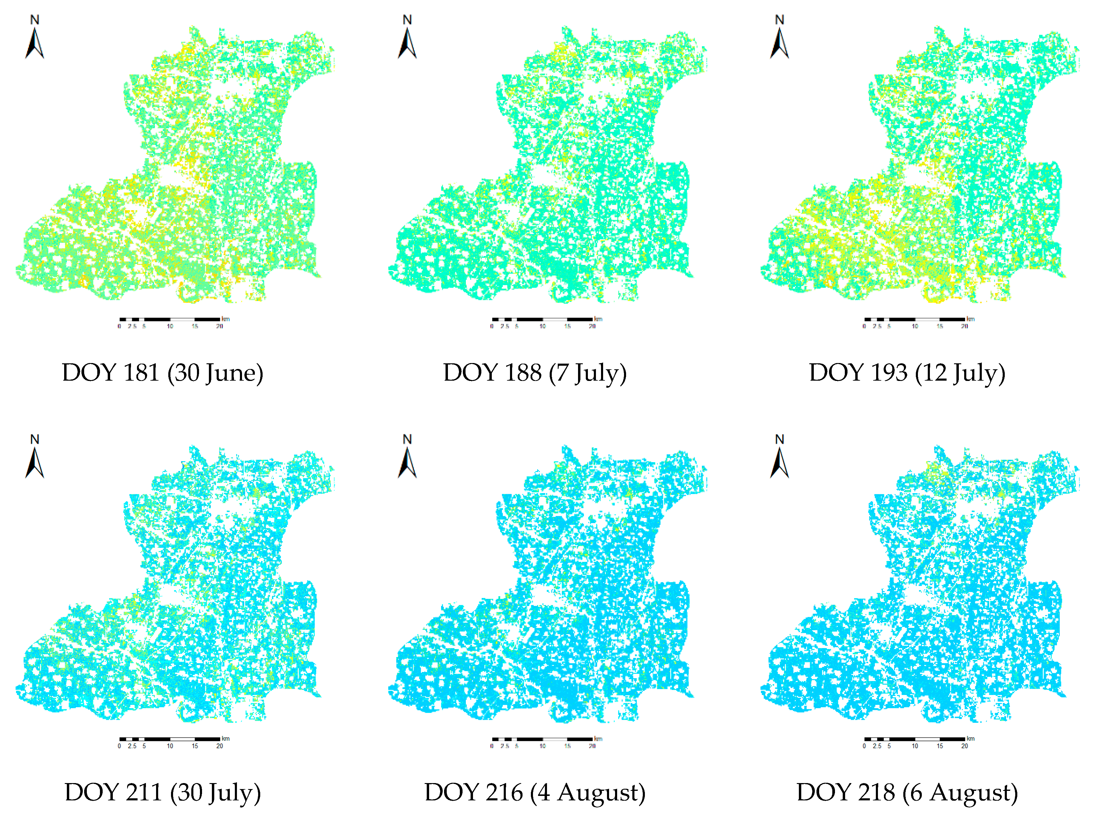
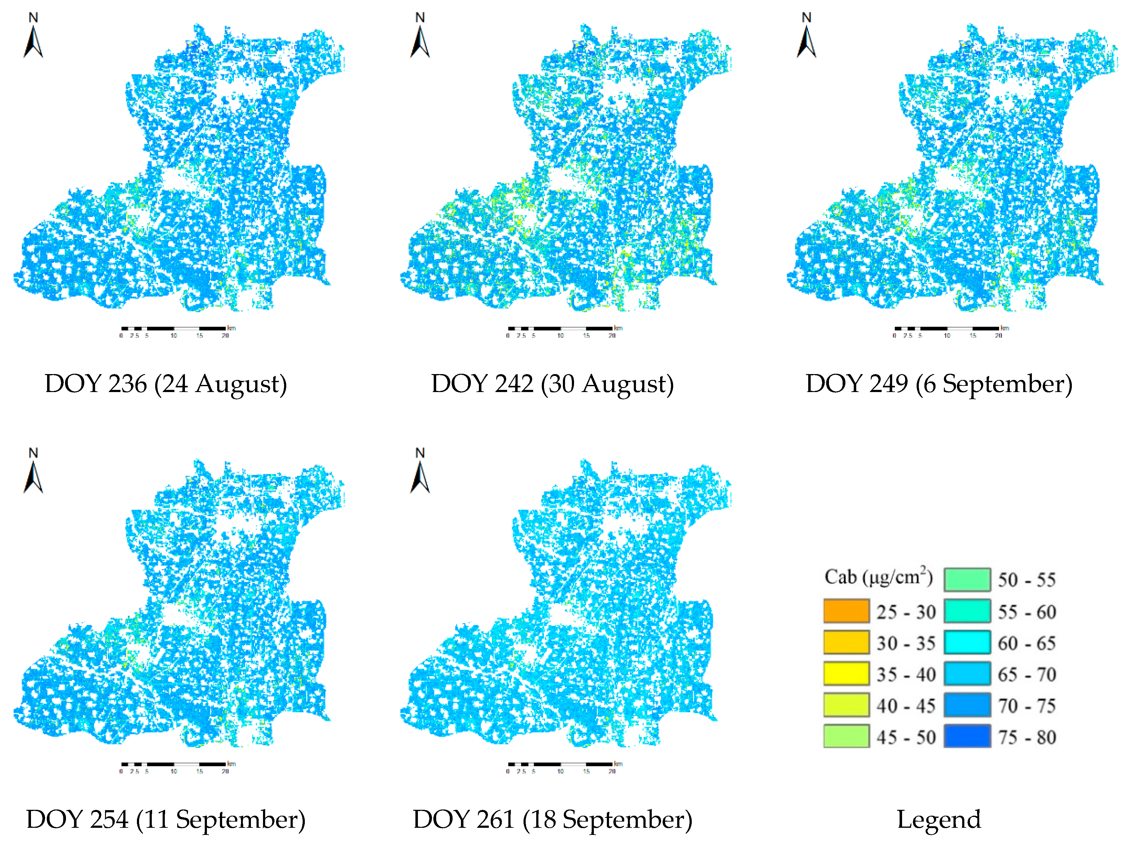
4.6. Monitoring the Corn Growth Behavior by Retrieved Time Series of LAI and Chlorophyll Content

Monitoring the changes in LAI and chlorophyll content during the growing season of corn is very important for achieving optimal crop productivity. We analyzed the corn growth behavior using the retrieved time series of LAI and chlorophyll content generated from this study. Figure 12 shows the time series of retrieved LAI and chlorophyll content during the growing season of corn in our study area, labeling the maximum estimate, minimum estimate, 1/4 quantiles, median, and 3/4 quantiles for this time series. The maximum and minimum are the ranging of estimated values, and the area between the 1/4 quantiles and the 3/4 quantiles to the median represent the dispersion of the retrieved LAI and chlorophyll content values. For the growing changing trend, Figure 12a indicates that LAI increased from DOY 181 to DOY 236 and decreased from DOY 236 to the end of the growing season, and the maximum LAI value was recorded on DOY 236. As shown in Figure 12b, chlorophyll content also peaked on DOY 236, rising steadily from DOY 181 to DOY 236 and falling steadily from DOY 236. For the spatial variation, the 1/4 quantiles and the 3/4 quantiles in Figure 12 illustrated that there was more variation for estimated LAI values than that of the estimated chlorophyll content values.

Figure 13 and Figure 14 show the maps of the retrieved LAI and chlorophyll content during the corn-growing season of 2017. It can be observed that the LAI increased from DOY 181 to DOY 218 and decreased from DOY 218 to DOY 261. In addition, the spatial and temporal heterogeneities of the chlorophyll content were higher than those of the LAI. More specifically, the LAI increased from a range of 0–0.5 on DOY 181 to 5.0–6.0 on DOY 236, and then decreased from a range of 5.0–6.0 on DOY 236 to 2.0–2.5 on DOY 261, which can be seen clearly from Figure 13. There was an obvious spatial heterogeneity in the LAI from DOY 236 to DOY 261, ranging from 2.0 to 6.0. Comparably, the chlorophyll content was stabilized at around 60 μg/cm² from DOY 211 to DOY 261 (Figure 14), except for DOY 181 to DOY 193, when they briefly increased.

5. Discussions

5.1. Remote Sensing Image Fusing by Kalman Filter

The 10-m spatial resolution of Sentinel-2 images allows for an improved representation of the spatial structure of corn planted areas. Unfortunately, the growing season of corn in the study area corresponds to rainy and hot climatic conditions, with frequent cloud cover, which result in few available Sentinel-2 images. For example, in our study, there were only five Sentinel-2 images for the growing season of 2017 (as seen in Figure 2), despite their five-day revisit period. The Kalman filter was used to solve this problem and synthetically increase the frequency of the images in this study. The fused remote sensing images with 10-m spatial resolution and daily temporal resolution are produced using our Kalman filter processing in this study. The comparative analysis in Section 4.3 revealed that there was high correlation between the fused image reflectance with Sentinel-2 image reflectance and in situ measured reflectance. There were still two issues that should be pointed out in this study. Firstly, there is big difference in the ground sampling distance (GSD) between MODIS image reflectance and Sentinel-2 image reflectance. Therefore, only the selected pure pixels of a corn planted area in a large homogeneous area were used for the state update and measurement update in Kalman filter. In the future, researchers should fuse the Sentinel-2 and Landsat images, or fuse the Sentinel-2 and Sentinel-3 images, which have a smaller spatial difference. Secondly, for the Kalman filter algorithm, the measurement update was done using the spatial information from high spatial resolution image (i.e., Sentinel-2 image in this study) reflectance. Unfortunately, there is generally insufficient measurement information for the remote sensing deficiency resulting from cloud, smog, rain, etc. [45]. This issue can be studied further in future.

5.2. Joint Retrieval of Corn Canopy LAI and Leaf Chlorophyll Using Co-Distributions

Canopy LAI and chlorophyll content are two very important parameters for corn growth monitoring. Generally speaking, a closed corn canopy is associated with high chlorophyll content commonly. In other words, corn canopy LAI and chlorophyll content are correlated. This correlation is mined to retrieve corn canopy LAI and chlorophyll content jointly in this study. For describing this correlation, Xu et al. [51] built up the matrices of VI pairs. For their selected VI pairs, one is sensitive to canopy LAI, and the other is sensitive to chlorophyll content. Referencing from the existent outstanding studies, we set up the co-distributions for joint retrieval in the whole corn-growing season. The co-distributions were built up in line with the in-situ measured LAI and chlorophyll content. The retrieved results indicated that both the retrieved LAI and chlorophyll content could be retrieved jointly and accurately. This joint retrieving method can be used to retrieve more crop parameters, such as LAI, chlorophyll content, equivalent water thickness (EWT), etc. Furthermore, this method can be extended to retrieve vegetation parameters efficiently in regional areas.

6. Conclusions

This study proposed a joint retrieval method for growing season corn canopy LAI and chlorophyll content by fusing the reflectances retrieved by Sentinel-2 and MODIS. This approach addresses the problem of missing Sentinel-2 images during vital crop growth stages caused by cloud occlusion. We applied a Kalman filter to produce a time series of high spatial resolution images for corn growth monitoring by taking advantage of the fine spatial structure of Sentinel-2 images while preserving the temporal resolution of MODIS images. In addition, the time series of images produced by the Kalman filtering technique was used to jointly retrieve LAI and chlorophyll content using their joint probability distributions as the inputs to the PROSAIL model. Furthermore, the retrieved time series of LAI and chlorophyll content were used to monitor the corn-growing behavior. Our results can be summarized as follows:

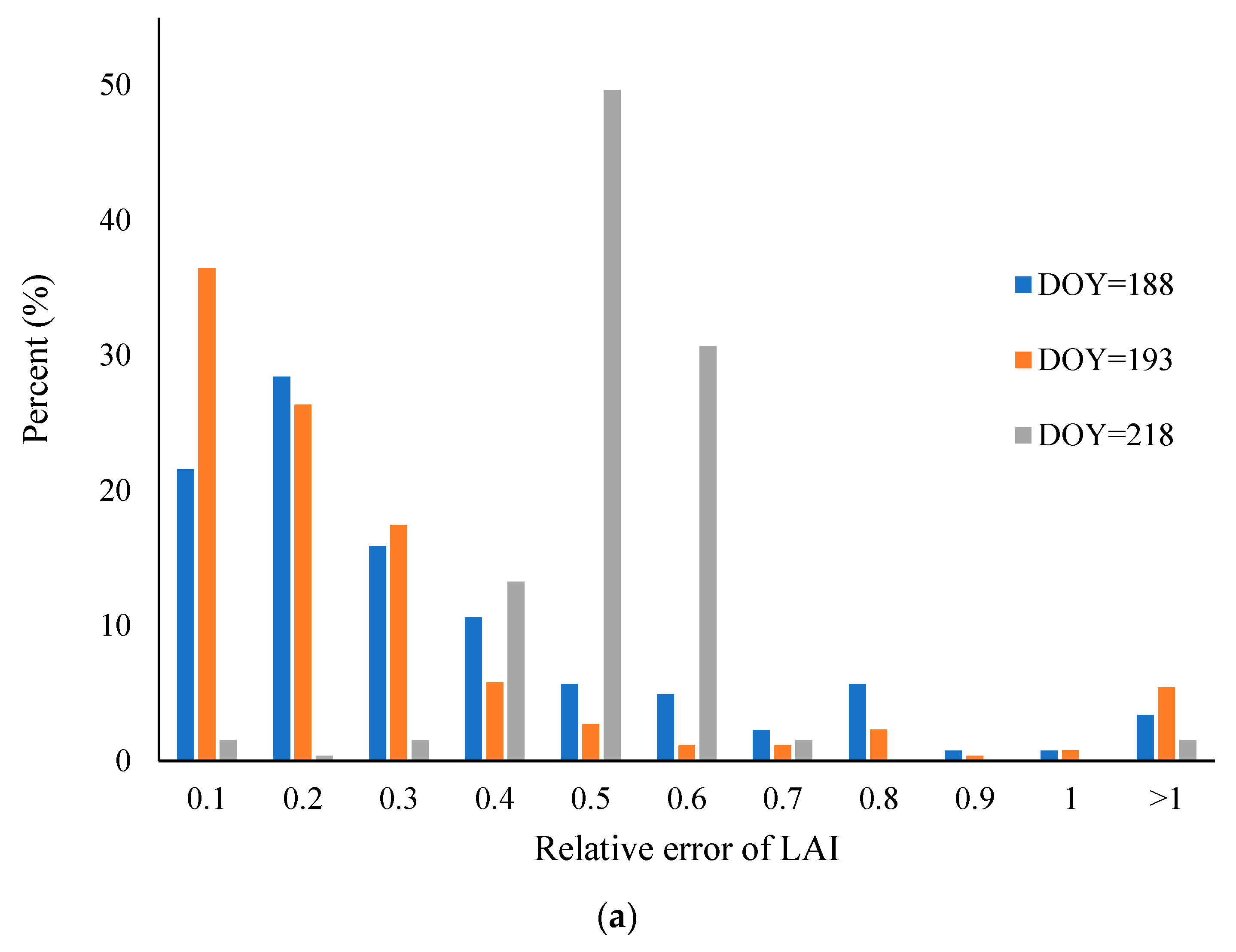
• The joint retrieval of LAI and chlorophyll content using the proposed joint probability distribution method demonstrated a good performance when compared with ground data. The R² value between the retrieved and measured parameters for four growth stages was about 0.6 for both LAI and chlorophyll content. Furthermore, the retrieval accuracy of the synthetic KF images was also assessed. The relative error between the retrieved and measured LAI and chlorophyll content were mainly distributed within the range of 0.1–0.2 μg/cm² and 0.0–0.3 μg/cm², respectively.
• Kalman filtering appeared to be a viable technique for producing continuous high-resolution reflectance images from synthesizing Sentinel-2 and MODIS reflectances. There was a significant correlation between the synthetic KF and the Sentinel-2 images both in the spatial structure and in their time series. There was almost no land cover structure difference between the Sentinel-2 and synthetic KF images, which could be confirmed by the fact that the points in the scatter plots for the blue, green, and red bands were close to the 1:1 line, while there was a bias on the scatter plot of the NIR band. In addition, the time series of synthetic blue, green, red, and NIR reflectances, NDVI, and EVI were all very similar to those of MODIS.
• Continuous KF reflectances were useful for monitoring the corn growth behavior during the entire growing season. Our analysis demonstrated that the LAI increased from DOY 181 (trefoil stage) to DOY 236 (filling stage), and then increased until the corn was harvested. Additionally, the results showed that chlorophyll content also increased from DOY 181 to DOY 236, and then remained stable until harvest. Compared with LAI, the chlorophyll content remained relatively stable during the growing season, ranging from 50 to 70 μg/cm².

In conclusion, the high temporal and spatial resolutions of synthetic remote sensing images produced through the Kalman filtering method proposed in this paper was able to capture the rapid LAI and chlorophyll content changes during the corn growing season. The study results are very promising, and could find applications in a number of areas, including crop growth monitoring, crop stress monitoring, crop yield forecast, and crop intervention. With the availability of Sentinel-1, Sentinel-2, Sentinel-3, and other new satellite remote sensing images, our approach can facilitate the fusion of all these satellite remote sensing data sources for the generation of synthetic time series images and for the joint retrieval of relevant crop canopy parameters. This will lead to improved high temporal and spatial resolution crop monitoring information to enable near real-time precision crop intervention and management. Our future efforts will be focused on the joint retrieval of other crop canopy parameters and apply the proposed method to other crops and other planted area of crops.

References

1. Yang, C.H.; Everitt, J.H.; Du, Q.; Luo, B.; Chanussot, J. Using high-resolution airborne and satellite imagery to assess crop growth and yield variability for precision agriculture. Proc. IEEE 2013, 101, 582–592. [Google Scholar] [CrossRef]
2. Tucker, C.J., Jr.; Elgin, J.H.; McMurtey, J.E., III; Fan, C.J. Monitoring corn and soybean crop development with hand-held radiometer spectral data. Remote Sens. Environ. 1979, 8, 237–248. [Google Scholar] [CrossRef]
3. Haboudane, D.; Miller, J.R.; Tremblay, N.; Zarco-Tejada, P.J.; Dextraze, L. Integrated narrow-band vegetation indices for prediction of crop chlorophyll content for application to precision agriculture. Remote Sens. Environ. 2002, 81, 416–426. [Google Scholar] [CrossRef]
4. Chen, J.M.; Black, T.A. Defining leaf area index for non-flat leaves. Plant Cell Environ. 2010, 15, 421–429. [Google Scholar] [CrossRef]
5. Fang, H.; Ye, Y.; Liu, W.; Wei, S.; Ma, L. Continuous estimation of canopy leaf area index (LAI) and clumping index over broadleaf crop fields: An investigation of the PASTIS-57 instrument and smartphone applications. Agric. For. Meteorol. 2018, 253–254, 48–61. [Google Scholar] [CrossRef]
6. Su, W.; Zhang, M.Z.; Bian, D.H.; Liu, Z.; Huang, J.X.; Wang, W.; Wu, J.Y.; Guo, H. Phenotyping of Corn Plants Using Unmanned Aerial Vehicle (UAV) Images. Remote Sens. 2019, 11, 2021. [Google Scholar] [CrossRef]
7. Gitelson, A.A.; Gritz, Y.; Merzlyak, M.N. Relationships between leaf chlorophyll content and spectral reflectance and algorithms for non-destructive chlorophyll assessment in higher plant leaves. J. Plant Physiol. 2003, 160, 271–282. [Google Scholar] [CrossRef]
8. Daughtry, C.S.T.; Walthall, C.L.; Kim, M.S.; Brown de Colstoun, E.; McMurtrey, J.E., III. Estimating corn leaf chlorophyll concentration from leaf and canopy reflectance. Remote Sens. Environ. 2000, 74, 229–239. [Google Scholar] [CrossRef]
9. GCOS. The Global Observing System for Climate: Implementation Needs (GCOS-200). World Meteorological Organization, 2016. Available online: https://library.wmo.int/opac/doc_num.php?explnum_id=3417 (accessed on 17 October 2018).
10. Huang, J.; Zhuo, W.; Li, Y.; Huang, R.; Sedano, F.; Su, W.; Dong, J.; Tian, L.; Huang, Y.; Zhu, D.; et al. Comparison of three remotely sensed drought indices for assessing the impact of drought on winter wheat yield. Int. J. Digit. Earth 2018. [Google Scholar] [CrossRef]
11. Huang, J.; Gómez-Dans, J.; Huang, H.; Ma, H.; Wu, Q.; Lewis, P.; Liang, S.; Chen, Z.; Xue, J.; Wu, Y.; et al. Assimilation of remote sensing into crop growth models: Current status and perspectives. Agric. For. Meteorol. 2019, 276–277, 107609. [Google Scholar] [CrossRef]
12. Merzlyak, M.N.; Gitelson, A.A.; Chivkunova, O.B.; Rakitin, V.Y. Non-destructive optical detection of pigment changes during leaf senescence and fruit ripening. Physiol. Plant. 2010, 106, 135–141. [Google Scholar] [CrossRef]
13. Veloso, A.; Mermoz, S.; Bouvet, A.; Toan, T.L.; Planells, M.; Dejoux, J.F.; Ceschia, E. Understanding the temporal behavior of crops using Sentinel-1 and Sentinel-2-like data for agricultural applications. Remote Sens. Environ. 2017, 199, 415–426. [Google Scholar] [CrossRef]
14. Huang, J.X.; Tian, L.Y.; Liang, S.L.; Ma, H.Y.; Becker-Reshef, I.; Su, W.; Huang, Y.B.; Zhang, X.D.; Zhu, D.H.; Wu, W.B. Improving winter wheat yield estimation by assimilation of the leaf area index from Landsat TM and MODIS data into the WOFOST model. Agric. For. Meteorol. 2015, 204, 106–121. [Google Scholar] [CrossRef] [Green Version]
15. Huang, J.X.; Sedano, F.; Huang, Y.B.; Ma, H.Y.; Li, X.L.; Liang, S.L.; Tian, L.Y.; Zhang, X.D.; Fang, J.L.; Wu, W.B. Assimilating a synthetic Kalman filter leaf area index series into the WOFOST model to improve regional winter wheat yield estimation. Agric. For. Meteorol. 2016, 216, 188–202. [Google Scholar] [CrossRef]
16. Chen, B.; Huang, B.; Xu, B. A hierarchical spatiotemporal adaptive fusion model using one image pair. Int. J. Digit. Earth 2017, 10, 639–655. [Google Scholar] [CrossRef]
17. Gao, F.; Masek, J.; Schwaller, M.; Hall, F. On the blending of the Landsat and MODIS surface reflectance: Predicting daily Landsat surface reflectance. IEEE Trans. Geosci. Remote Sens. 2006, 44, 2207–2218. [Google Scholar]
18. Zhu, X.; Chen, J.; Gao, F.; Chen, X.; Masek, J.G. An enhanced spatial and temporal adaptive reflectance fusion model for complex heterogeneous regions. Remote Sens. Environ. 2010, 114, 2610–2623. [Google Scholar] [CrossRef]
19. Zhu, X.; Helmer, E.H.; Gao, F.; Liu, D.; Chen, J.; Lefsky, M.A. A flexible spatiotemporal method for fusing satellite images with different resolutions. Remote Sens. Environ. 2016, 172, 165–177. [Google Scholar] [CrossRef]
20. Zhao, Y.; Huang, B.; Song, H.A. A robust adaptive spatial and temporal image fusion model for complex land surface changes. Remote Sens. Environ. 2018, 208, 42–62. [Google Scholar] [CrossRef]
21. Roy, D.P.; Ju, J.; Lewis, P.; Schaaf, C.; Gao, F.; Hansen, M.; Lindquist, E. Multi-temporal MODIS-Landsat data fusion for relative radiometric normalization, gap filling, and prediction of Landsat data. Remote Sens. Environ. 2008, 112, 3112–3130. [Google Scholar] [CrossRef]
22. Wang, Q.; Atkinson, P.M. Spatio-temporal fusion for daily Sentinel-2 images. Remote Sens. Environ. 2018, 204, 31–42. [Google Scholar] [CrossRef] [Green Version]
23. Huang, B.; Song, H. Spatiotemporal reflectance fusion via sparse representation. IEEE Trans. Geosci. Remote Sens. 2012, 50, 3707–3716. [Google Scholar] [CrossRef]
24. Mathieu, P.; O’Neill, A. Data assimilation: From photon counts to Earth System forecasts. Remote Sens. Environ. 2008, 112, 1258–1267. [Google Scholar] [CrossRef]
25. Sedano, F.; Kempeneers, P.; Hurtt, G. A Kalman filter-based method to generate continuous time series of medium-resolution NDVI images. Remote Sens. 2014, 6, 12381–12408. [Google Scholar] [CrossRef]
26. Darvishzadeh, R.; Skidmore, A.; Schlerf, M.; Atzberger, C. Inversion of a Radiative Transfer Model for Estimating Vegetation LAI and Chlorophyll in a Heterogeneous Grassland. Remote Sens. Environ. 2008, 112, 2592–2604. [Google Scholar] [CrossRef]
27. Viña, A.; Gitelson, A.A.; Nguy-Robertson, A.L.; Peng, Y. Comparison of different vegetation indices for the remote assessment of green leaf area index of crops. Remote Sens. Environ. 2011, 115, 3468–3478. [Google Scholar] [CrossRef]
28. Li, Z.H.; Xu, X.G.; Jin, X.J.; Gu, X.H. Retrieval of LAI and leaf chlorophyll content from remote sensing data by agronomy mechanism knowledge to solve the ill-posed inverse problem. SPIE Remote Sens. 2014, 9239, 92391Q. [Google Scholar]
29. Jacquemoud, S.; Verhoef, W.; Baret, F.; Bacour, C.; Zarcotejada, P.J.; Asner, G.P.; François, C.; Ustin, S.L. PROSPECT+SAIL models: A review of use for vegetation characterization. Remote Sens. Environ. 2009, 113, S56–S66. [Google Scholar] [CrossRef]
30. Verhoef, W. Light scattering by leaf layers with application to canopy reflectance modeling: The SAIL model. Remote Sens. Environ. 1984, 16, 125–141. [Google Scholar] [CrossRef] [Green Version]
31. Jacquemoud, S.; Baret, F. PROSPECT: A model of leaf optical properties spectra. Remote Sens. Environ. 1990, 34, 75–91. [Google Scholar] [CrossRef]
32. Baret, F.; Jacquemoud, S.; Guyot, G.; Leprieur, C. Modeled analysis of the biophysical nature of spectral shifts and comparison with information content of broad bands. Remote Sens. Environ. 1992, 41, 133–142. [Google Scholar] [CrossRef]
33. Li, Z.H.; Jin, X.L.; Wang, J.H.; Yang, G.J.; Nie, C.W.; Xu, X.G.; Feng, H.K. Estimating winter wheat (triticum aestivum) LAI and leaf chlorophyll content from canopy reflectance data by integrating agronomic prior knowledge with the PROSAIL model. Int. J. Remote Sens. 2015, 36, 2634–2653. [Google Scholar] [CrossRef]
34. Jay, S.; Maupas, F.; Bendoula, R.; Gorretta, N. Retrieving lai, chlorophyll and nitrogen contents in sugar beet crops from multi-angular optical remote sensing: Comparison of vegetation indices and prosail inversion for field phenotyping. Field Crop. Res. 2017, 210, 33–46. [Google Scholar] [CrossRef]
35. Botha, E.J.; Leblon, B.; Zebarth, B.; Watmough, J. Non-destructive estimation of potato leaf chlorophyll from canopy hyperspectral reflectance using the inverted PROSAIL model. Int. J. Appl. Earth Obs. Geoinf. 2007, 9, 360–374. [Google Scholar] [CrossRef]
36. Darvishzadeh, R.; Matkan, A.A.; Ahangar, A.D. Inversion of a radiative transfer model for estimation of rice canopy chlorophyll content using a lookup-table approach. IEEE J. Sel. Top. Appl. Earth Obs. Remote Sens. 2012, 5, 1222–1230. [Google Scholar] [CrossRef]
37. Rivera, J.P.; Verrelst, J.; Leonenko, G.; Moreno, J. Multiple cost functions and regularization options for improved retrieval of leaf chlorophyll content and LAI through inversion of the PROSAIL model. Remote Sens. 2013, 5, 3280–3304. [Google Scholar] [CrossRef]
38. Duan, S.B.; Li, Z.L.; Wu, H.; Tang, B.H.; Ma, L.; Zhao, E.Y.; Li, C.R. Inversion of the PROSAIL model to estimate leaf area index of maize, potato, and sunflower fields from unmanned aerial vehicle hyperspectral data. Int. J. Appl. Earth Obs. Geoinf. 2014, 26, 12–20. [Google Scholar] [CrossRef]
39. Fang, H.; Li, W.; Wei, S.; Jiang, C. Seasonal variation of leaf area index (LAI) over paddy rice fields in NE China: Intercomparison of destructive sampling, LAI-2200, digital hemispherical photography (DHP), and AccuPAR methods. Agric. For. Meteorol. 2014, 198–199, 126–141. [Google Scholar] [CrossRef]
40. Darvishzadeh, R.; Atzberger, C.; Skidmore, A.; Schlerf, M. Mapping grassland leaf area index with airborne hyperspectral imagery: A comparison study of statistical approaches and inversion of radiative transfer models. ISPRS J. Photogramm. Remote Sens. 2011, 66, 894–906. [Google Scholar] [CrossRef]
41. Markwell, J.; Osterman, J.C.; Mitchell, J.L. Calibration of the Minolta SPAD-502 leaf chlorophyll meter. Photosynth. Res. 1995, 46, 467–472. [Google Scholar] [CrossRef]
42. European Space Agency (ESA). The Sentinel Application Platform (SNAP), A Common Architecture for all Sentinel Toolboxes Being Jointly Developed by Brockmann Consult, Array Systems Computing and C-S. 2017. Available online: http://step.esa.int/main/download/ (accessed on 1 April 2017).
43. Zhuo, W.; Huang, J.; Li, L.; Zhang, X.; Ma, H.; Gao, X.; Huang, H.; Xu, B.; Xiao, X. Assimilating Soil Moisture Retrieved from Sentinel-1 and Sentinel-2 Data into WOFOST Model to Improve Winter Wheat Yield Estimation. Remote Sens. 2019, 11, 1618. [Google Scholar] [CrossRef]
44. Kalman, R.E. A new approach to linear filtering and prediction problems. J. Basic Eng. Trans. 1960, 82, 35–45. [Google Scholar] [CrossRef]
45. Zhang, M.Z.; Zhu, D.H.; Su, W.; Huang, J.X.; Zhang, X.D.; Liu, Z. Harmonizing Multi-Source Remote Sensing Images for Summer Corn Growth Monitoring. Remote Sens. 2019, 11, 1266. [Google Scholar] [CrossRef]
46. Baret, F.; Buis, S. Estimating Canopy Characteristics from Remote Sensing Observations: Review of Methods and Associated Problems. In Advances in Land Remote Sensing; Springer: Dordrecht, The Netherlands, 2008. [Google Scholar]
47. Weiss, M.; Baret, F. S2ToolBox Level 2 Products. Version 1.1. Date Issued: 05 February 2016. Available online: step.esa.int/docs/extra/ATBD_S2ToolBox_L2B_V1.1.pdf (accessed on 17 October 2018).
48. Su, W.; Huang, J.X.; Liu, D.S.; Zhang, M.Z. Retrieving corn canopy leaf area index from multitemporal Landsat imagery and terrestrial LiDAR data. Remote Sens. 2019, 11, 572. [Google Scholar] [CrossRef]
49. Combal, B.; Baret, F.; Weiss, M.; Trubuil, A.; Macé, D.; Pragnère, A.; Myneni, R.; Knyazikhin, Y.; Wang, L. Retrieval of canopy biophysical variables from bidirectional reflectance: Using prior information to solve the ill-posed inverse problem. Remote Sens. Environ. 2002, 84, 1–15. [Google Scholar] [CrossRef]
50. Locherer, M.; Hank, T.; Danner, M.; Mauser, W. Retrieval of seasonal leaf area index from simulated EnMAP data through optimized LUT-based inversion of the PROSAIL model. Remote Sens. 2015, 7, 10321–10346. [Google Scholar] [CrossRef]
51. Xu, M.Z.; Liu, R.G.; Chen, J.M.; Liu, Y.; Shang, R.; Ju, W.M.; Wu, C.Y.; Huang, W.J. Retrieving leaf chlorophyll content using a matrix-based vegetation index combination approach. Remote Sens. Environ. 2019, 224, 60–73. [Google Scholar] [CrossRef]
Figure 1. Location (a) of the study area (b) including sample plots, and schematic diagram of the sampling pattern in each plot (c).
Remotesensing 11 02409 g001
Figure 2. Calendar of remote sensing data acquisitions and field measurements, expressed in day of year (DOY). Notes: The top line shows the acquisition dates of five Sentinel-2 images (square symbol); the middle line indicates the acquisition dates of four field measurements (plus symbol); the bottom line represents the acquisition dates of 13 MOD09GA images (triangle symbol).
Remotesensing 11 02409 g002
Figure 3. The workflow for fusing two kinds images and joint retrieval for leaf area index (LAI) and chlorophyll content.
Remotesensing 11 02409 g003
Figure 4. Flowchart for fusing Sentinel-2 and MODIS images. For each time-step, A is the transition model for the time update of x k and x k + 1 , z k is a Sentinel-2 observation, and x ^ k is the final estimate in this state. The final estimates would be smoothed by forward and backward modes (Sedano et al., 2014).
Remotesensing 11 02409 g004
Figure 5. Scheme of co-distribution between LAI and chlorophyll content in the filling stage (Stage 3). There are 15,000 random numbers; the LAI range is used to restrict the chlorophyll content range. Referenced from reference (Weiss and Baret, 2016).
Remotesensing 11 02409 g005
Figure 6. The restriction and optimization process using joint probability distributions. (a) is the scatter plot between LAI and chlorophyll content, (b,c) are the statistical estimates of LAI and chlorophyll content (μg/cm2) with an optimized parameter range, parameter range, and mathematical Gaussian distribution, respectively.
Remotesensing 11 02409 g006
Figure 7. Subsets of MODIS, Sentinel-2, and Kalman filtered (KF) images in four spectral bands at day of year (DOY) 193. (a,e,i,m) are MODIS reflectances on blue, green, red and NIR bands respectively; (b,f,j,n) are Sentinel-2 reflectances on blue, green, red and NIR bands respectively; (c,g,k,o) are KF reflectances on blue, green, red and NIR bands respectively; (d,h,l,p) are the scatter plots of Sentinel-2 and KF reflectances on blue, green, red and NIR bands respectively.
Remotesensing 11 02409 g007
Figure 8. Time-series reflectances for blue (a), green (b), red (c), near infrared (NIR) (d) bands, and normalized difference vegetation index (NDVI) (e) and Enhanced Vegetation Index (EVI) (f) vegetation indexes. The purple lines are MODIS reflectances, the blue lines are KF reflectances, and the orange triangles are Sentinel-2 reflectances.
Remotesensing 11 02409 g008
Figure 9. Comparison of KF and field-measured reflectance on DOY 193 (a), DOY 236 (b), and DOY 242 (c). The dotted lines are Sentinel-2 reflectances, the dashed lines are KF reflectances, and the solid lines are in situ measured reflectances.
Remotesensing 11 02409 g009
Figure 10. Relation between KF and Sentinel-2 reflectance with field reflectance measured on DOY 193. (a) is the correlation between KF and in-situ measured reflectance, (b) is the correlation between KF and Sentinel-2 reflectance, (c) is the correlation between Sentinel-2 and in-situ measured reflectance.
Remotesensing 11 02409 g010
Figure 11. The relative error of retrieval of LAI (a) and chlorophyll content (b) using synthetic KF and Sentinel-2 images
Remotesensing 11 02409 g011aRemotesensing 11 02409 g011b
Figure 12. Time series of retrieved LAI (a) and chlorophyll content (b) using synthetic KF images during the growing season of corn of 2017.
Remotesensing 11 02409 g012aRemotesensing 11 02409 g012b
Figure 13. Study area LAI maps for the corn-growing season of 2017.
Remotesensing 11 02409 g013aRemotesensing 11 02409 g013b
Figure 14. Study area chlorophyll content maps for the corn-growing season of 2017.
Remotesensing 11 02409 g014aRemotesensing 11 02409 g014b