A Cuboid Model for Assessing Surface Soil Moisture

Abstract

This study proposes a cuboid model for soil moisture assessment. In the model, the three edges were the meteorological, soil, and vegetation feature parameters highly related to soil moisture, and the edge lengths represented the degree of influence of each feature parameter on soil moisture. Soil moisture is assessed by the cuboid diagonal, which is referred to as the cuboid soil moisture index (CSMI) in this paper. The model was applied and validated in the Huang-Huai-Hai Plain. The results showed that (1) the difference in land surface temperature between day and night (ΔLST), land surface water index (LSWI), and accumulated precipitation (AP) were most closely correlated with soil moisture observation data in our study area, and were therefore selected as soil, crop, and meteorological system parameters to participate in CSMI calculations, respectively. (2) CSMI-1, with a cuboid length coefficient of 2/1/2, was the best model. The correlation of soil moisture derived from CSMI-1 with observed values was 0.64, 0.60, and 0.52 at depths of 10 cm, 20 cm, and 50 cm, respectively. (3) CSMI-1 had good applicability to the evaluation of soil moisture under different vegetation coverage. When the normalized difference vegetation index (NDVI)was 0–0.7, CSMI-1 was highly correlated with soil moisture at a significance level of 0.01. (4) The three-dimensional (3D) CSMI model can be easily converted to a two-dimensional (2D) model to adapt to different surface conditions (as long as the weight coefficient of one parameter is set to 0). Irrigation information (if available) can be considered as artificial recharge precipitation added in the AP to improve the accuracy of soil moisture inversion. This study provides a reference for soil moisture inversion using optical remote sensing images by integrating soil, vegetation, and meteorological feature parameters.

1. Introduction

Soil moisture is an important component of the water, energy, and biogeochemical cycle [1,2,3], and is of great significance to related research on water resources management, agricultural production, and climate change [4,5]. Soil moisture monitoring can be divided into three categories based on data acquisition methods: site measurement, simulation and assimilation, and soil moisture inversions based on remote sensing data [3]. Among them, the precision of soil moisture observed by stations is high, but because of the discrete characteristics of observation stations, the soil moisture observed by stations cannot reflect the temporal and spatial continuous variation characteristics of soil moisture at a regional scale. The soil moisture data simulated by assimilation models have continuity in space and time, but the accuracy of simulation largely depends on the selection of parameterization schemes and parameterization process. Besides, assimilation models require a large number of input parameters, reducing their practicability. Remote sensing has the remarkable advantage of large-scale synchronous observation and reflects the continuous change information of the earth’s surface in time and space [6], which makes it an important data source for soil moisture inversion research.

Research into soil moisture retrieval based on remote sensing began in the 1960s [3,6]. In early investigations of soil moisture inversions, researchers used single factors to establish inversion models, such as optical reflectance [7,8,9], thermal infrared [10], and microwave-based methods [11,12,13]. Researchers directly established models of the relationship between a single factor (such as reflectance, brightness temperature, thermal inertia, or backscattering coefficient) and soil moisture [14] or used a single factor to construct an index to indirectly reflect soil moisture. For example, the normalized difference vegetation index (NDVI) [15], vegetation condition index (VCI) [16,17,18,19,20], normalized difference water index (NDWI) [21], global vegetation moisture index (GVMI) [22], land surface water index (LSWI) [23], visible and shortwave infrared drought index (VSDI) [24], and normalized multi-band drought index (NMDI) [25] are calculated using optical reflectance, while the land surface temperature (LST) [26,27], normalized difference temperature index (NDTI) [28], and temperature condition index (TCI) [16] are calculated using thermal infrared bands. The indices mentioned above are often used to monitor surface drought and soil moisture.

Recently, researchers have used multiple factors, such as the combination of visible and thermal infrared bands or visible and microwave bands, to establish inversion models [29,30] or construct comprehensive indexes to monitor soil moisture [31]. For example, Goward et al. found that when the vegetation coverage in the study area changed widely, the surface temperature and NDVI formed triangular or trapezoidal shapes on the scatter plot; therefore, they put forward the concept of soil moisture contours [32]. Gillies and Carlson constructed a universal triangle method for evaluation of surface soil moisture content [33]. Satellite-derived surface radiant temperature and a vegetation index were associated in an inverse modeling scheme and found to fit the observed data well. Subsequently, Sandholt et al. constructed a temperature vegetation drought index (TVDI) based on the characteristic space, which takes into account the thermal infrared characteristics on the basis of optical characteristics and can better characterize the soil moisture status [9]. D. Zhang et al. proposed a new soil moisture index, the temperature rising rate vegetation dryness index (TRRVDI) based on the surface temperature-vegetation index triangle method, in which the instantaneous temperature was replaced with the mid-morning land surface temperature rising rate [34]. This index had better coefficient of determination at 19 meteorological stations in Spain than the one-time LST and vegetation index and reduced the uncertainty associated with the data; however, it requires substantial ground data and is complex to calculate [3]. Amani et al. synthesized vegetation and soil characteristics to construct a temperature-vegetation-soil moisture dryness index (TVMDI) based on the perpendicular vegetation index (PVI), LST, and soil moisture (SM) [35]. In this model, SM and PVI were calculated based on the red-near infrared feature space, after which, the LST was added to construct the three-dimensional (3D) feature space and the TVMDI was obtained according to the relationship of the body diagonals. The correlation coefficient between the TVMDI and measured soil moisture was 0.65. In addition to the combination of soil and vegetation features, there are soil moisture indices that have been proposed by combining visible and microwave bands. For example, X. Zhang et al. presented a synthesis method that divided soil moisture into a baseline and change value, in which the baseline was the lowest state of soil moisture in the observation period and the change value depended on the influence of meteorological elements, such as precipitation and evapotranspiration [36]. This model accurately estimated the daily soil moisture content of 1 km resolution in the Xinjiang province with a mean square error of the model inversion results and ground measured values of 3.99%, indicating it can be used for high-precision soil moisture retrieval. It is important to note that the meteorological elements in this study only participated in the construction of soil water model as auxiliary variables in the form of rainfall correction factors, which means few studies have investigated the synthesis of soil, vegetation, and meteorological conditions.

Soil moisture content is influenced by many factors, including soil characteristics, vegetation coverage, and meteorological conditions, which results in it having high spatial heterogeneity. In the existing multi-factor soil moisture inversion research, two elements of vegetation, soil and meteorological elements, are usually considered comprehensively, but three elements are not considered at the same time. In theory, considering the meteorological, soil, and vegetation systems synthetically can improve the accuracy of soil moisture inversion. Therefore, this study was conducted to build a comprehensive inversion model of soil moisture by integrating meteorological, soil, and vegetation systems to indicate the soil moisture status. Specifically, this research proposes a cuboid model for soil moisture assessment, which is referred to as the cuboid soil moisture index (CSMI) in this paper. The main purpose of this paper is to introduce the model and construction process of the CSMI. Researchers can follow the methodology of this work to calculate the CSMI for their own study area by customizing the parameters and the length coefficients of the three edges of the cuboid model according to the meteorological, soil, and vegetation characteristics of their study area.

2. Materials and Methods

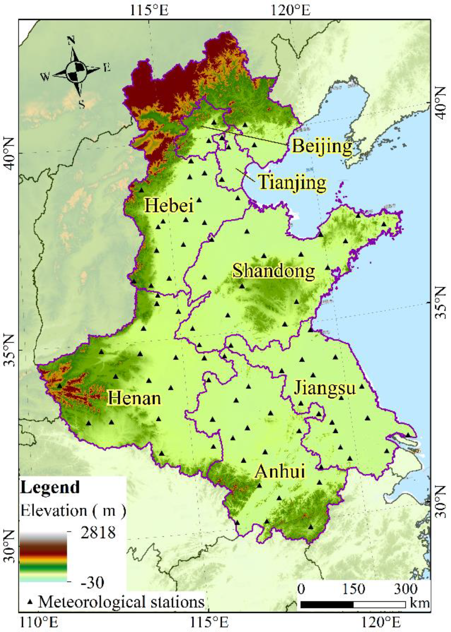
2.1. Study Areas

The Huang-Huai-Hai Plain is located between 32°–40°N and 114°–121°E, spanning seven provinces (cities) including Beijing, Tianjin, Hebei, Shandong, Henan, Anhui, and Jiangsu (Figure 1). It is the second largest plain and one of the most important agricultural production bases in China, with double cropped wheat-maize rotations. Most of the Huang-Huai-Hai Plain has a warm temperate monsoon climate, with obvious changes in four seasons. The plain is dry and cold in winter, while it is hot and rainy in summer, and subject to drought and less rain in spring. The difference in annual precipitation and the uneven distribution of soil moisture lead to frequent drought and flood disasters in this area, among which, drought is the most prominent, with the highest frequency occurring in spring, early summer, and autumn. In addition, the water resources in the Huang-Huai-Hai Plain are relatively scarce, the per capita water resources are only 15% of those in the whole country, and groundwater is seriously overexploited. Therefore, accurate monitoring of soil moisture in this region is of great significance for agricultural production and water resources management.

2.2. Data

The data used in this study include remote sensing data, site observation data, and auxiliary data. Remote sensing data included surface reflectance products (MOD09A1) and surface temperature products (MOD11A2) from the MODIS (Moderate-Resolution Imaging Spectroradiometer) satellite and daily precipitation rate data sets from the TRMM (Tropical Rainfall Measuring Mission) satellite. Site observation data included the daily dataset of surface climate data and soil moisture data. Both were obtained from the China Meteorological Data Network (http://data.cma.cn), but the corresponding observation stations were not the same. The former was from basic weather stations and included daily air pressure, temperature, precipitation, evaporation, relative humidity, wind direction, wind speed, sunshine hours, and 0 cm ground temperature data. The latter was from agrometeorological stations. Strict quality checks and controls, including extreme value checks and time consistency checks, were conducted on the basic weather station, after which, 90 meteorological stations in Huang-Huai-Hai Plain that had complete and continuous data and covered nearly the whole study area were selected. In addition, the nearest agrometeorological station to the basic meteorological station was selected. Finally, we selected 58 agrometeorological stations that had both soil moisture data and daily climate data. Two of these were in Beijing, 15 in Hebei, 14 in Henan, 16 in Jiangsu, and 11 in Anhui. Soil moisture data mainly covered the growing season of winter wheat, including 10 cm, 20 cm, and 50 cm soil moisture. The acquisition time of remote sensing data and site observation data was from March to May 2010. Auxiliary data were the provincial administrative boundary and land use land cover map of our study area in 2010.

Table 1. Data description.

Name	Spatial Resolution	Temporal Resolution	Source	Utility
Surface reflectance (MOD09A1)	500 m	8-day	United States Geological Survey (USGS)	Model input
Land surface temperature (MOD11A2)	1000 m	8-day	USGS	Model input
Daily precipitation rate (TRMM3B42)	0.25°	1-day	National Aeronautics and Space Administration (NASA)	Model input
Daily Data Set of Surface Climate Data (temperature, evaporation, precipitation)	−	1-day	China meteorological information center (CMIC)	Model input
Soil Moisture	−	10-day	CMIC	Accuracy verification
Land use land cover map	1000 m	yearly	Resource and environment data cloud platform, institute of geographic science and natural resources research	Extracting the distribution of cultivated land
Provincial boundary	−	−	National fundamental geographic information system in national geomatics center of China	Obtaining the boundary of the research area

describes the attributes, sources, and uses of the data employed in this study.

Data preprocessing included: (1) using MODIS Reprojection Tools (MRT) software to re-projected MOD09A1 and MOD11A2 data as a WGS84 coordinate system and saved them as tiff format. (2) Using the ENVI (Environment for Visualizing Images) software to re-project TRMM3B42 data as a WGS84 coordinate system and re-sample it to 1 km spatial resolution. (3) Based on the QC (quality control) file of MOD11A2 and MOD09A1, surface reflectance and temperature data that were not affected by cloud and aerosol in Huang-Huai-Hai Plain were extracted. (4) The ten-day average temperature (Tave), average evaporation (Eave), and accumulated precipitation (AP) were calculated by using the daily average temperature, evaporation, and precipitation data.

2.3. Method

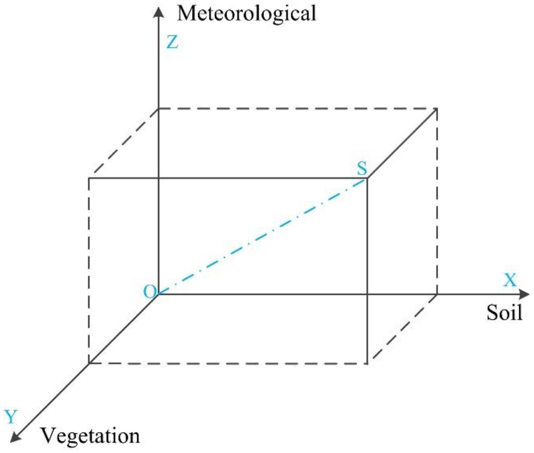
2.3.1. Cuboid Soil Moisture Index (CSMI)

Considering the meteorological, soil system, and vegetation system, three parameters related to soil moisture were placed in a three-dimensional space to construct a cuboid soil moisture index (CSMI), in which the X-axis was used to represent the soil system, the Y-axis was used to represent the vegetation system, and the Z-axis was used to represent the meteorological system. The parameters represented by the three coordinate axes are positively correlated with soil moisture, and they are unified into dimensionless parameters in the range of 0–1. The edge length coefficient was then determined according to the contribution rate of each coordinate axis to soil moisture. Figure 2 shows the schematic diagram of CSMI and Equation (1) shows the formula of the model.

$$CSMI=\sqrt{\frac{{aX}^2+{bY}^2+{cZ}^2}{a^2+b^2+c^2}}$$

(1)

where X, Y, and Z represent the three axes of the cuboid and a, b, and c are edge length coefficients determined according to the contribution rate of each coordinate axis to soil moisture. Pixels near point O have the lowest moisture values (0), while those at the other end of the OS (point S) have the maximum moisture values.

2.3.2. Cuboid Soil Moisture Index Calculation

Our technological flowchart is shown in Figure 3. There are mainly three steps: Firstly, building the candidate soil, vegetation and meteorological feature parameters set and a feature parameter which have the highest correlation with soil moisture for each axis of the cuboid is selected. Secondly, normalizing the selected feature parameters to 0–1 and making them positively correlated with soil moisture, and lastly, determining the edge length coefficient based on the analytic hierarchy process (AHP) and calculating CSMI according to Formula 1.

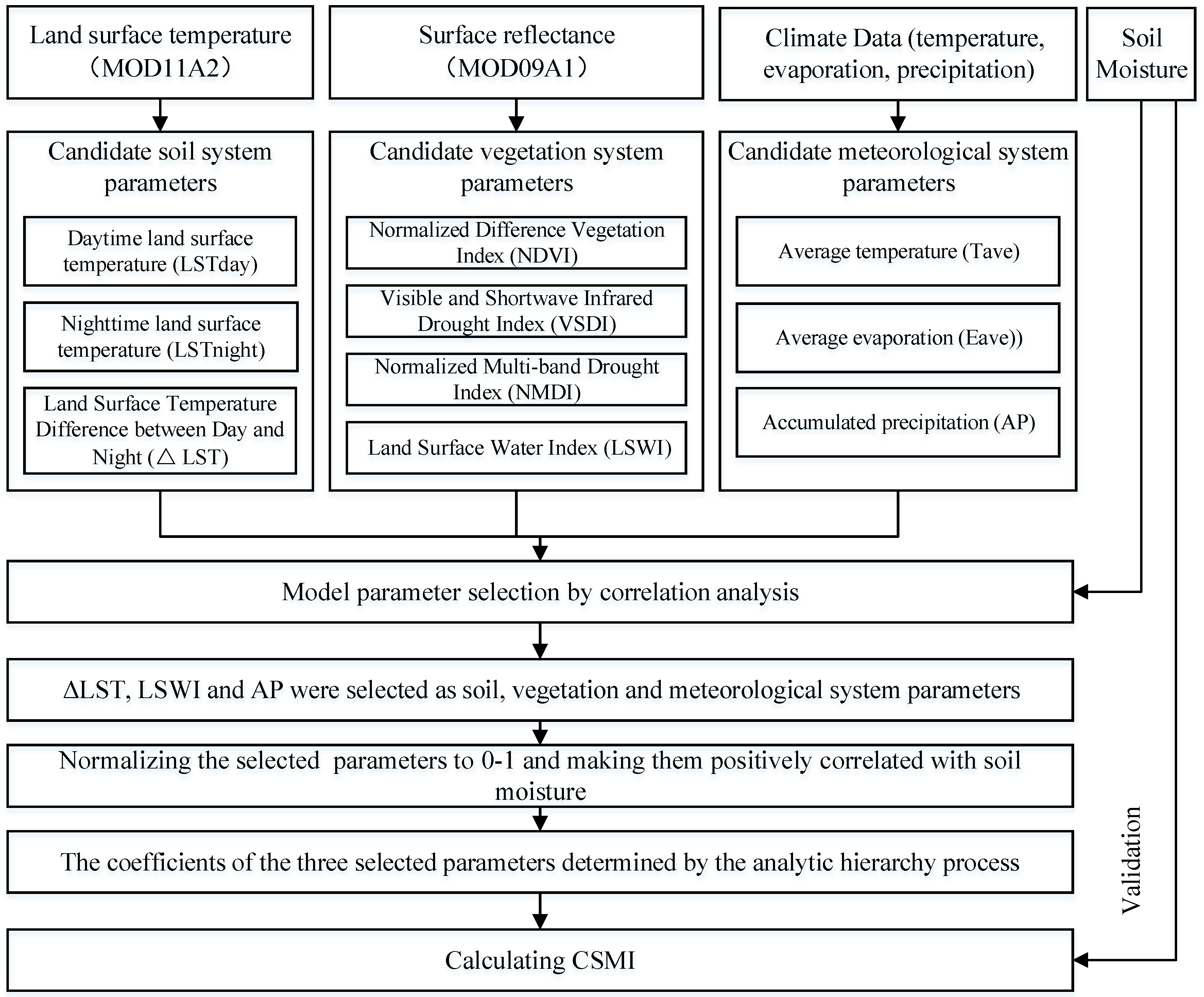
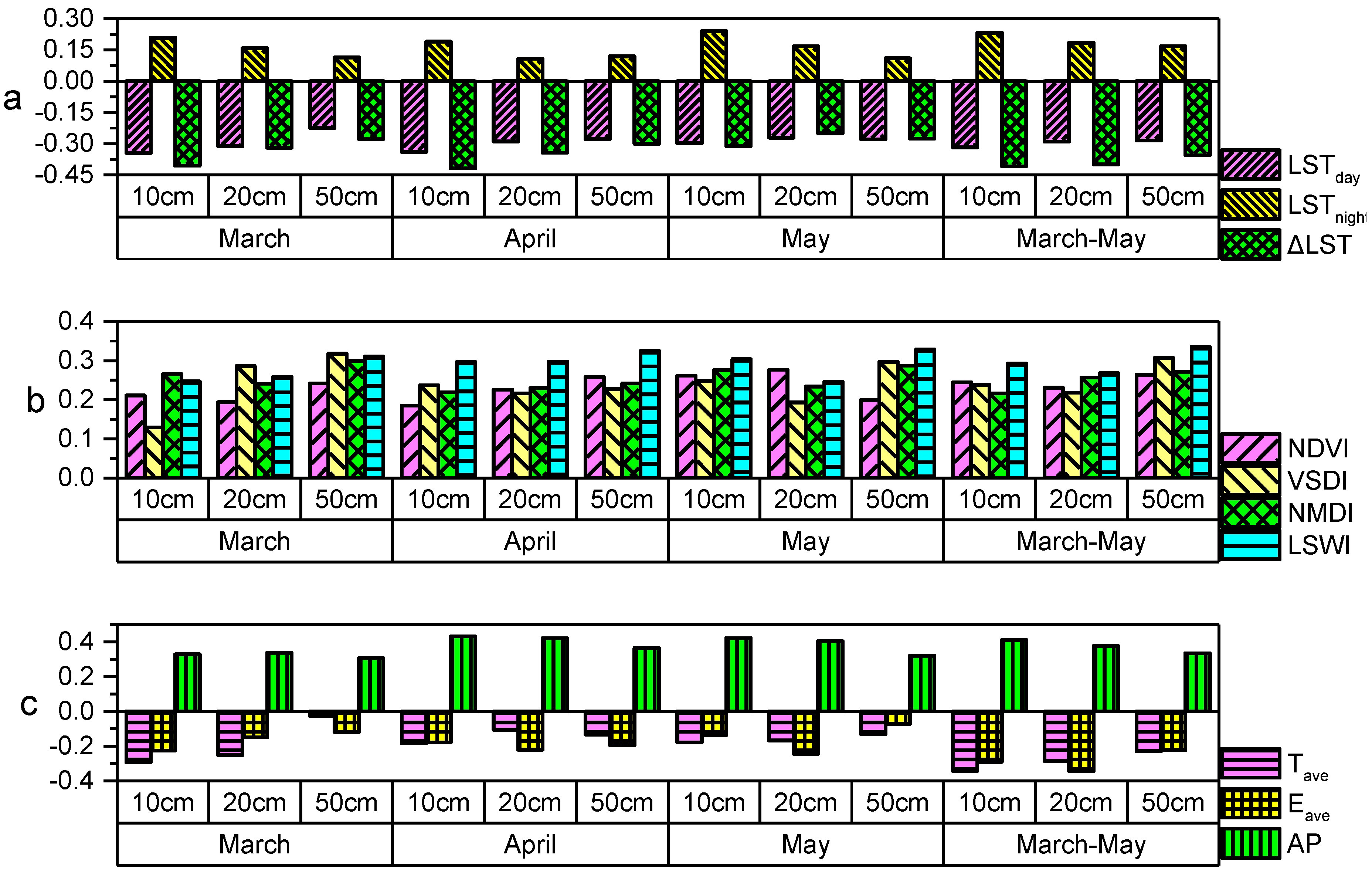
Model Parameter Selection

There are three parameters in the model corresponding to soil, vegetation, and meteorological systems. The candidate soil system parameters considered in this study included the surface temperature of observation stations during the day (${\mathrm{LST}}_{\mathrm{day}}$) and at night (${\mathrm{LST}}_{\mathrm{night}}$) and the difference in land surface temperature between day and night ($\mathrm{\Delta }\mathrm{LST}$). The candidate vegetation system parameters included the normalized difference vegetation index (NDVI) [15], the visible and shortwave infrared drought index (VSDI) [24], the normalized multi-band drought index (NMDI) [25], and the land surface water index (LSWI) [23], while the meteorological system parameters included Tave, Eave, and AP. The correlation coefficients between soil moisture data at different depths (10 cm, 20 cm, and 50 cm) and candidate parameters were calculated, after which, candidate parameters with the highest correlation in soil, vegetation, and meteorological systems with measured soil moisture were selected to participate in modeling. The main influence factors of soil moisture at different depths are different [37,38,39]. For example, with the increase of soil depth, the influence of surface climatic factors on soil moisture is weakened. We calculated the relationship between soil moisture at different depths and candidate feature variables and selected the feature parameters with the highest correlation with soil moisture at different depths to participate in the calculation of CSMI. So that CSMI can better reflect soil moisture at different depths.

$$\mathrm{\Delta }\mathrm{LST}={LST}_{day}-{LST}_{night}$$

(2)

where, ${LST}_{day}$ and ${LST}_{night}$ represent the land surface temperature during the day and night respectively, from the MODIS LST products (MOD11A2). $\mathrm{\Delta }\mathrm{LST}$ represents the change of day and night temperature.

$$\mathrm{NDVI}=\frac{\left(R_{nir}-R_{red}\right)}{\left(R_{nir}+R_{red}\right)}$$

(3)

$$\mathrm{VSDI}=1-\left[\left(R_{swir}-R_{blue}\right)-\left(R_{red}-R_{blue}\right)\right]$$

(4)

$$\mathrm{NMDI}=\frac{\left[R_{860nm}-\left(R_{1640nm}-R_{2130nm}\right)\right]}{\left[R_{860nm}+\left(R_{1640nm}-R_{2130nm}\right)\right]}$$

(5)

$$\mathrm{LSWI}=\frac{\left(R_{nir}-R_{swir}\right)}{\left(R_{nir}+R_{swir}\right)}$$

(6)

where, $R_{red}$, $R_{nir}$, $R_{swir}$, and $R_{blue}$ are the spectral reflectance values of surface red, near infrared, shortwave infrared, and blue bands respectively, and $R_{860nm}$, $R_{1640nm}$, and $R_{2130nm}$ represent the spectral reflectance at 860, 1640, and 2130 nm, respectively. The value of NDVI is between −1 and 1. If soil moisture is suitable for vegetation growth, better vegetation growth is associated with a greater corresponding NDVI value. Conversely, if the soil moisture is low, the vegetation will grow poorly under the influence of water stress, and the corresponding NDVI value will be smaller. The VSDI (LSWI) is positively correlated with soil moisture, with a larger VSDI (LSWI) indicating higher soil water content. NMDI is inversely proportional to soil moisture, with a higher NMDI value being associated with smaller soil moisture and vice versa.

Parametric Standardization

The three selected parameters had different units, so it was necessary to standardize them. To accomplish this, the maximum-minimum standardization method (Equation (7)) was used for dimensionless processing, and the range of values was between 0 and 1 after standardization.

$$\mathrm{P}=\frac{p_i-min\left(p\right)}{max\left(p\right)-min\left(p\right)}$$

(7)

where, $p$ is one of the three selected parameters, $\mathrm{P}$ is the value of the ith data after standardization, $p_i$ is the original value of the ith data, and $max\left(p\right)$ and $min\left(p\right)$ are the maximum and minimum values of parameter $p$, respectively.

Edge Length Coefficient Determination

The edge length coefficient was determined based on the analytic hierarchy process (AHP) [40]. It is one of multi criteria decision-making methods and is widely used in many fields, such as groundwater potential mapping [41], and crop growth condition monitoring [42], etc. The basic principle of this method, which quantifies the process of qualitative analysis, is to divide the complex problems to be solved into several simple problems. Different problems and corresponding solutions can form a hierarchical structure, after which, the relative importance of all indicators can be judged layer by layer and a judgment matrix can be constructed. The eigenvector of the judgment matrix is then calculated, and the component of the eigenvector is the weight of the corresponding elements in single order. The ranking of the importance weight of the lowest index to the highest overall objective can finally be obtained.

In this study, the five-level scale method was used to determine the relative importance (

Table 2. Five-Level Scaling Method and Its Meaning.

Scale Value	Compare Factors i and j
1	Factor i is as important as j, and the scale value is 1.
3	Factor i is obviously more important than j, and the scale value is 3
5	Factor i is much more important than j, and the scale value is 5.
2, 4	The median value of the above two adjacent judgments
Reciprocal of 1–5	The scale value of factor i compared with factor j is equal to the reciprocal of the scale value of factor j compared with factor i.

). Referring to the correlation between feature parameters and soil moisture, we constructed three sets of judgment matrices to further improve the credibility of the final results (

Table 3. Judgment matrix.

CSMI		X	Y	Z
CSMI-1	X	1	2	1
	Y	1/2	1	1/2
	Z	1	1/2	1
CSMI-2	X	1	2	1/2
	Y	1/2	1	1/3
	Z	2	3	1
CSMI-3	X	1	3	1/2
	Y	1/3	1	1/4
	Z	2	4	1

Note: CSMI refers to Cuboid Soil Moisture Index. X, Y, and Z correspond to the soil system, vegetation system, and meteorological system, respectively.

) and used a consistency test to judge whether there were contradictions among the weights of each index [40,43]. In the consistency test, the maximum eigenvalue of the judgment matrix was first calculated and recorded as ${\mathsf{\lambda }}_{\max },$ after which the consistency index (CI) was calculated according to $\mathrm{CI}=\left({\mathsf{\lambda }}_{\max }-\mathrm{n}\right)/\left(\mathrm{n}-1\right)$, where n is the number of indicators in the hierarchical subsystem. Finally, the random consistency ratio (CR) was calculated according to CR = CI/RI, where RI is the random consistency index. When the CR is less than 0.10, the judgment matrix has satisfactory consistency and it is acceptable when the CR is less than 1 [44]. Otherwise, the judgment matrix needs to be reconstructed.

3. Results

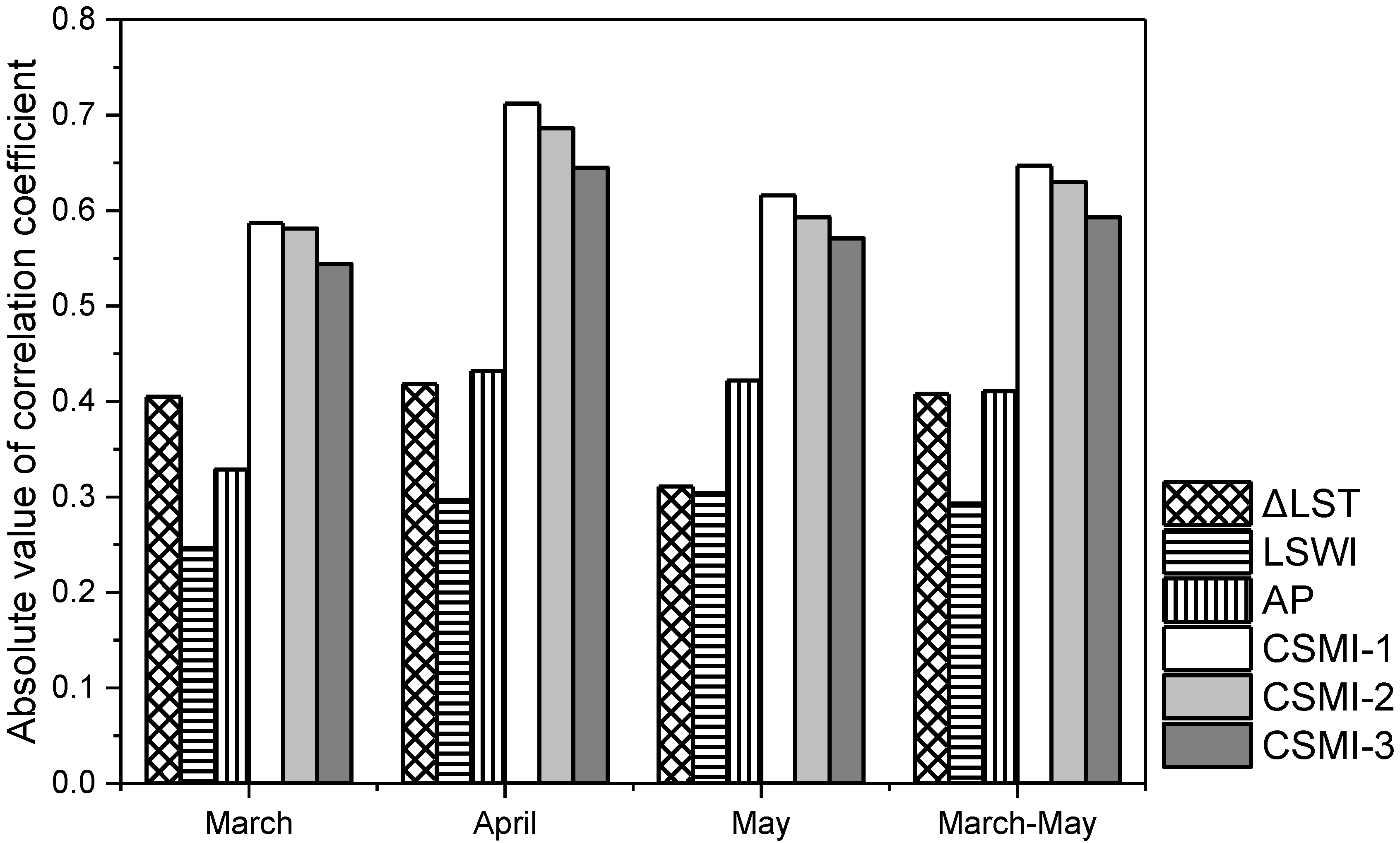
3.1. Model Parameters and Edge Length Coefficient

The correlation coefficients between candidate parameters and measured soil moisture at different depths is shown in Figure 4. From the figure, we can see that (1) from March to May in the Huang-Huai-Hai region, the parameters of the soil system were best correlated with the 10 cm soil moisture in most cases, followed by the 20 cm soil moisture, and finally the 50 cm soil moisture. These findings indicate that the accuracy of monitoring soil moisture by surface temperature decreases with increased depth. The surface temperature in daytime is negatively correlated with soil moisture, while the surface temperature at night is positively correlated with soil moisture. The ΔLST had the highest correlation with the measured soil moisture, followed by the LSTday. (2) The vegetation system parameters were best correlated with 50 cm soil moisture in most cases, followed by 20 cm soil moisture, and finally, 10 cm soil moisture. Among them, LSWI had the best correlation with soil moisture at different depths as a whole. The relationship between vegetation parameters and soil moisture was best in May, followed by April and March. (3) In terms of meteorological system parameters, the correlation between AP and soil moisture at different depths was best, followed by Eave and Tave. The correlation coefficient between AP and soil moisture was highest in April, followed by May. The correlation between AP and soil moisture at 10 cm was highest, followed by 20 cm and 50 cm. These findings indicate that the correlation between AP and soil moisture in each month decreased with increased soil depth. Therefore, ΔLST, LSWI, and AP were selected as soil, vegetation, and meteorological system parameters to participate in CSMI calculation, respectively. To ensure that the three parameters were positively correlated with soil moisture, the three parameters of the final cuboid model were calculated by Equations (8)–(10).

$$\mathrm{X}=1-\mathrm{\Delta }{LST}_s=1-\frac{\mathrm{\Delta }{LST}_i-\mathrm{\Delta }{LST}_{min}}{\mathrm{\Delta }{LST}_{max}-\mathrm{\Delta }{LST}_{min}}$$

(8)

$$\mathrm{Y}={LSWI}_s=\frac{{LSWI}_i-{LSWI}_{min}}{{LSWI}_{max}-{LSWI}_{min}}$$

(9)

$$\mathrm{Z}={AP}_s=\frac{{AP}_i-{AP}_{min}}{{AP}_{max}-{AP}_{min}}$$

(10)

where $\mathrm{\Delta }{LST}_s$, ${LSWI}_s$, and ${AP}_s$ are new standardized values of $\mathrm{\Delta }{LST}_i$, ${LSWI}_i$, and ${AP}_i$ respectively, $\mathrm{\Delta }{LST}_i$, ${LSWI}_i$, and ${AP}_i$ denote the original values of each parameter, $\mathrm{\Delta }{LST}_{max}$, ${LSWI}_{max}$, and ${AP}_{max}$ are the maximum values of the three selected parameters, and $\mathrm{\Delta }{LST}_{min}$, ${LSWI}_{min}$, and ${AP}_{min}$ represent the minimum values of the three selected parameters.

The coefficients of the three selected parameters determined by the analytic hierarchy process are shown in

Table 4. Edge length coefficients determined by the Analytic Hierarchy Process (AHP) method.

CSMI	a	b	c	CR
CSMI-1	0.4	0.2	0.4	0.0032
CSMI-2	0.3	0.2	0.5	0.0088
CSMI-3	0.3	0.1	0.6	0.0176

. Based on these three sets of judgment matrices, we obtained three sets of coefficients and their consistency test results. The results of three tests showed that CR was less than 0.10 and passed the consistency test. Therefore, the three combinations of the a/b/c edge length coefficients were finally determined to be 2/1/2, 3/2/5, and 3/1/6, respectively.

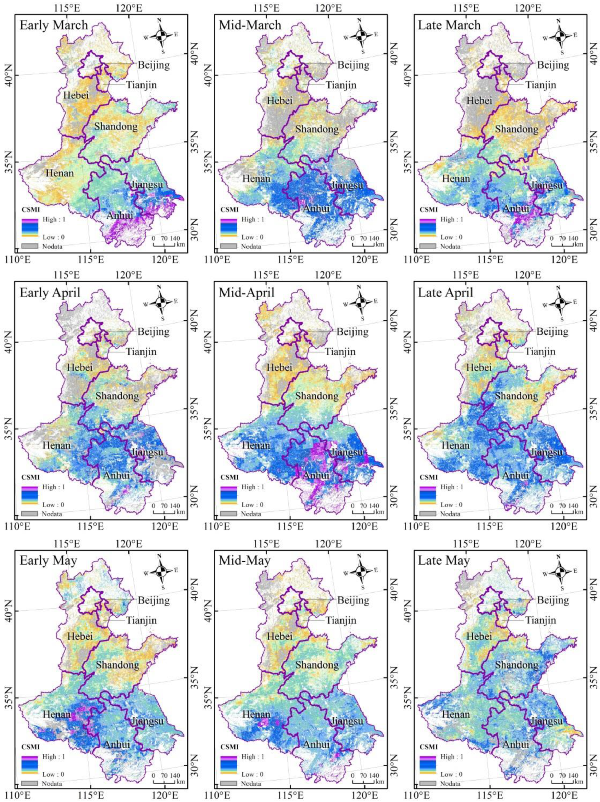
3.2. CSMI of Study Area

The correlation coefficients between CSMI calculated based on different edge length coefficients and measured soil moisture are shown in

Table 5. Pearson correlation coefficients between CSMI and soil moisture at different depths.

CSMI	Soil Moisture
	10 cm	20 cm	50 cm
CSMI-1	0.647 **	0.600 **	0.518 **
CSMI-2	0.630 **	0.585 **	0.507 **
CSMI-3	0.593 **	0.554 **	0.482 **

Note: ** indicates a significant correlation at the 0.01 level (bilateral).

. During the crop growing season in the Huang-Huai-Hai region, the correlation coefficients between CSMI-1 and soil moisture at different depths were largest, followed by CSMI-2 and CSMI-3. The correlation coefficients between CSMI-1 and soil moisture at different depths were above 0.51. These findings indicated that the edge length coefficient of the model 2/1/2 was the optimal edge length coefficient in our study area.

The cultivated land area was extracted from the land use land cover map of the Huang-Huai-Hai Plain, and CSMI-1 of cultivated land in Huang-Huai-Hai Plain was calculated using precipitation rate data sets from the TRMM satellite and land surface reflectance and temperature data from the MODIS satellite. The results are shown in Figure 5. Soil moisture in the south Huang-Huai-Hai region was higher than in the north, with Anhui and Jiangsu provinces having the highest soil moisture, followed by Henan and Shandong provinces, and Beijing-Tianjin-Hebei provinces having the lowest soil moisture. In early March, Anhui Province had the highest soil moisture value, followed by Jiangsu Province and Shandong Province. The soil moisture in Shandong Province decreased in mid-March and early April, while it increased in the southeastern Henan Province. In late March and late April, soil moisture in Anhui, Jiangsu, and Henan provinces was higher, while it was lower in Shandong, Beijing, Tianjin, and Hebei. In mid-April and mid-May, soil moisture in Anhui and Jiangsu provinces was highest, followed by Henan and Shandong provinces, while it was still low in Beijing, Tianjin, and Hebei. In early May and late May, soil moisture in Beijing, Tianjin, and Hebei showed an upward trend, especially in northern Hebei.

4. Discussion

4.1. Impacts of Edge Length Coefficient on CSMI

The absolution values of correlation coefficients between three CSMIs and soil moisture at a depth of 10 cm with those of the three selected parameters and soil moisture at a depth of 10 cm were compared (Figure 6). Overall, the correlation between CSMI and soil moisture was higher than that between single parameter and soil moisture. The correlation between CSMI and soil moisture was highest in April followed by May, while it was lowest in March. The edge length coefficients of CSMI-1, CSMI-2, and CSMI-3 were 2/1/2, 3/2/5, and 3/1/6, respectively; therefore, the ranking of the edge length coefficients of the three individual parameters was AP = ΔLST > LSWI in CSMI-1 and AP > ΔLST > LSWI in both CSMI-2 and CSMI-3. The ranking of correlation coefficients of the three individual parameters and soil moisture was ΔLST > AP > LSWI in March, AP ≈ ΔLST > LSWI in April, and AP > ΔLST ≈ LSWI in May, respectively. In CSMI-1, the ranking of the edge length coefficient of the three individual parameters was highly consistent with the ranking of correlation coefficients of the three individual parameters and soil moisture. Moreover, the ranking of correlation coefficients of the three individual parameters and soil moisture in CSMI-1 was the same as the ranking of the edge length coefficient of the three individual parameters in April. These findings explain why CSMI-1 was more closely related to soil moisture than CSMI-2 and CSMI-3 and why CSMI-1 had best relationship with soil moisture in April.

Based on the above analyses, the three edge length coefficients in the model had a great influence on the results of the CSMI calculation. In this study, the three edge length coefficients from March to May were the same, but the effects of climate, soil, and vegetation on soil moisture varied among different months. According to the influence of climate, soil, and vegetation on soil moisture in different months, the accuracy of CSMI can be improved by dynamically adjusting the coefficients of the three parameters monthly.

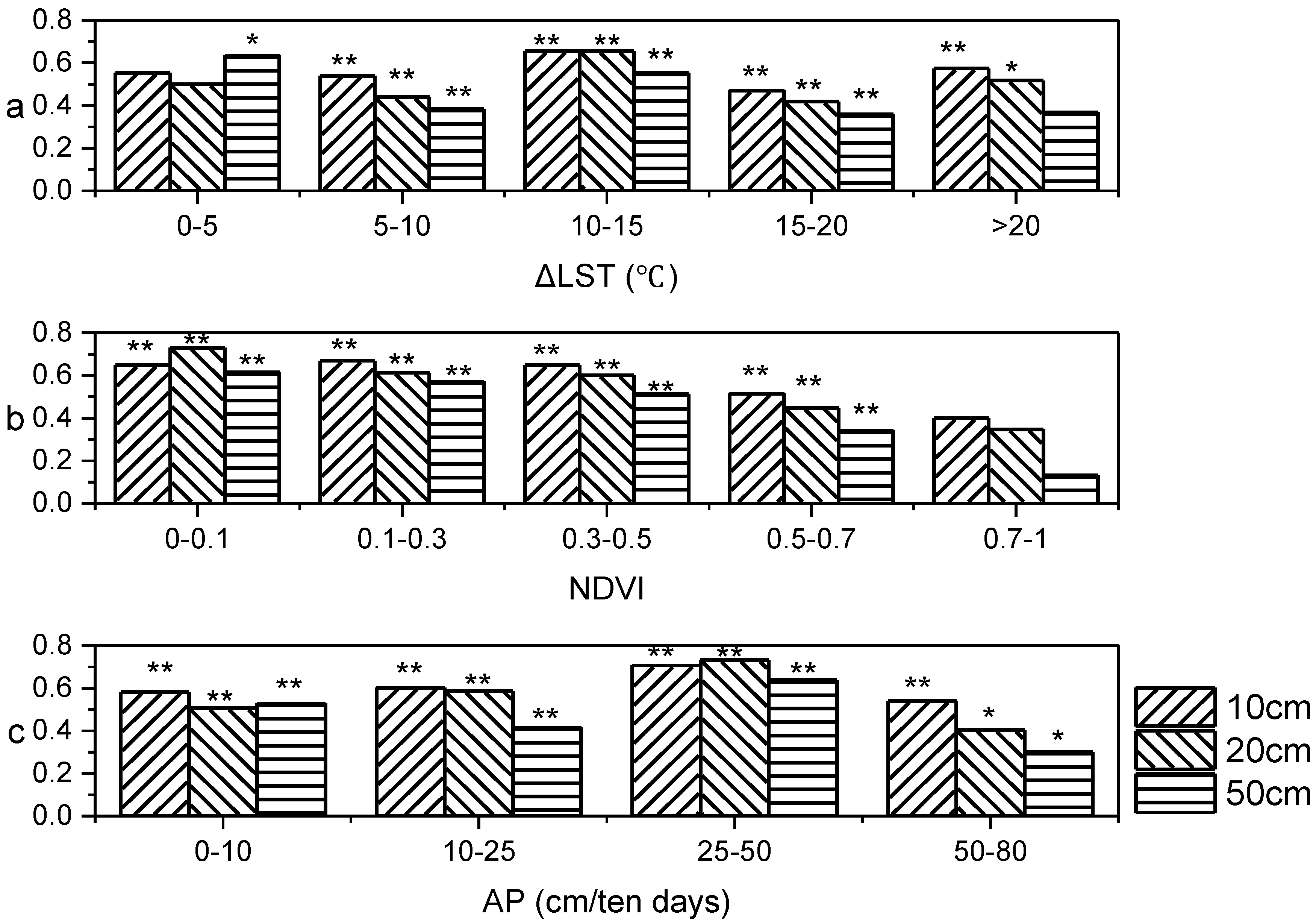
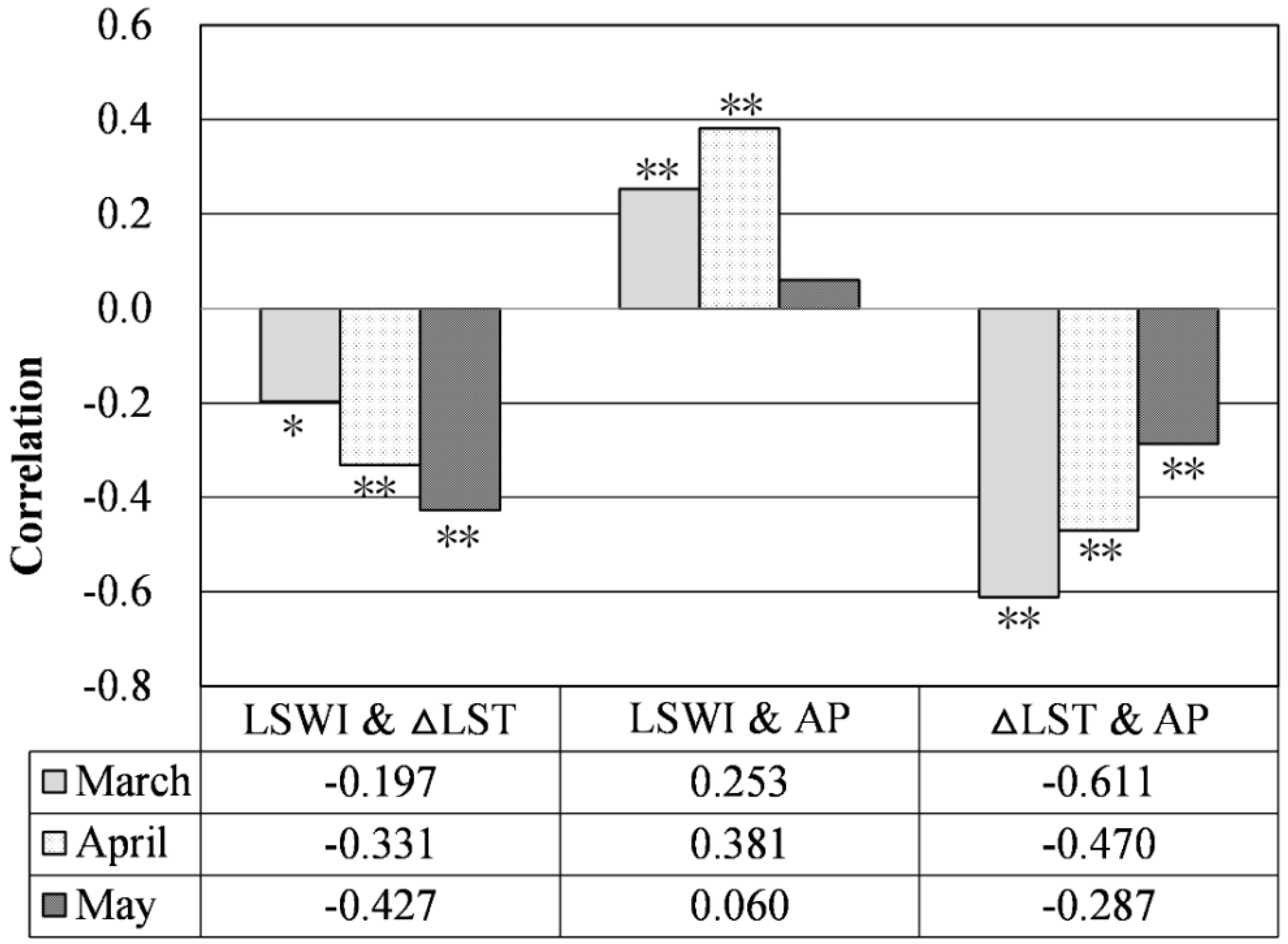
4.2. Impacts of Surface Temperature Difference, Crop Growth, and Accumulated Precipitation on CSMI

To analyze the effects of surface temperature differences, crop growth, and accumulated precipitation on the accuracy of the CSMI model, we divided the ΔLST into five grades with 5 °C, 10 °C, 15 °C, and 20 °C as break points, NDVI into five grades with 0.1, 0.3, 0.5, and 0.7 as break points, and AP into four grades with 10, 25, and 50 cm/ten days as break points. The correlation coefficients between CSMI-1 and soil moisture at different levels of ΔLST, NDVI, and AP were then calculated. As shown in Figure 7, the correlation coefficients between CSMI-1 and soil moisture varied among different levels of ΔLST, NDVI, and AP. Under most cases, CSMI-1 had the best correlation with soil moisture at 10 cm, followed by 20 cm and 50 cm. In other words, the correlation coefficient between CSMI-1 and soil moisture generally decreased as soil depth increased, which is consistent with the findings in Table 5. The correlation coefficients of CSMI-1 and soil moisture showed no obvious trend with the change of ΔLST (Figure 7a). Regardless of the NDVI and AP levels, the correlation between CSMI-1 and soil moisture at different depths was greatest when ΔLST was 10–15 °C. When NDVI was lower than 0.7, CSMI-1 was highly correlated with soil moisture at a significance of 0.01, which indicated that CSMI had good applicability to the evaluation of soil moisture under different vegetation coverage (Figure 7b). When NDVI was larger than 0.7, the correlation coefficients between CSMI-1 and soil moisture at different depths were below 0.4 and did not pass the significance test. One possible reason for this was that the stations we used in this study were agrometeorological stations, and there were few observation data for stations with NDVI values higher than 0.7. AP and soil moisture at different depths were highly correlated at a statistical significance level of α = 0.05 (Figure 7c). Regardless of the NDVI and ΔLST levels, the correlation between CSMI-1 and soil moisture at different depths was greatest when AP was 25–50 cm.

4.3. Limitations and Potential Improvement of This Study

Firstly, in this paper, for selection of feature parameters of the CSMI model, only the correlation between candidate characteristic parameters and soil moisture was considered, and the correlation between parameters was not considered. We found that correlation among the three parameters varied with time (Figure 8). The three parameters had the highest correlation in April, followed by March, and finally, May. The correlation between ΔLST and AP was the highest in April and May, and the correlation between LSWI and ΔLST was the highest in June. It may affect the setting of weights to some extent. In future studies, we will consider selecting characteristic parameters with high correlation with soil moisture and low correlation among variables to calculate CSMI index.

Second, this study is limited in that the spatial and temporal heterogeneity of soil moisture is not considered when determining the edge length coefficients of the three axes of the CSMI model. However, different land cover types, such as bare soil and vegetation, may have different soil moisture. The same type of land use, such as vegetation, also differs in soil moisture at different growth stages. When determining the edge length coefficient, the condition of the underlying surface can be fully considered, and the edge length coefficient can be adjusted dynamically, according to changes in the underlying surface to ensure that the coordinate axes of the cuboid model can play an effective role and further improve the accuracy of the model. If the edge length coefficient of any of the three parameters in the cuboid model is set to 0, the three-dimensional cuboid model will be transformed into a two-dimensional model. For example, when the coefficient of crop parameter is set to 0, the effect of vegetation cover on soil moisture is not considered, and the model is suitable for soil moisture inversion in bare soil. When the coefficient of soil parameter is set to 0, the effect of bare surface on soil moisture is not considered, and the model is suitable for the inversion of surface moisture in the case of dense vegetation coverage.

Another limitation is that, although precipitation can indicate soil water recharge, the changes in soil moisture caused by factors such as irrigation by human activities are not considered in this study. If irrigation information can be considered as artificial recharge precipitation added in the Z axis of CSMI, the accuracy of the model can be further improved. However, detailed irrigation information (such as irrigation location, time, and intensity) is very scarce, especially in large-scale research areas [45]. Therefore, in theory, the current CSMI model without considering irrigation information has better applicability in rain-fed areas.

Finally, in this study, we constructed and validated the CSMI model based on the data of 58 agrometeorological stations in the Huang-Huai-Hai Plain in 2010. Larger regional validations, as well as those for other vegetation types (such as forests and grasslands) in other years have not yet been conducted. Among the many remote sensing parameters that have been developed to describe soil moisture, there are no accepted optimal parameters [3]. The performance of the same parameter differs among regions [46]. The main purpose of this article is to propose a model and construction process of the CSMI. Researchers can follow the methodology of this work, select the parameters of the three edges of the cuboid model suitable for their study area, and determine the length coefficients of the three edges according to the meteorological, soil and vegetation characteristics of their study area.

4.4. Significance of This Study

The importance of this study lies in two aspects:

Firstly, our study results indicate that integrating soil, vegetation, and meteorological feature parameters can improve the accuracy of soil moisture inversion. The relationship between feature parameters (such as AP, ΔLST, and LSWI) and soil moisture varies with time and soil depth. It may be a development direction in the future to build an adaptive soil moisture inversion model in which the weights of the three axes in CSMI varies with time. In general, the correlation coefficient between CSMI with soil moisture decreases with the increase of soil depth. Thus, it is more difficult to improve the precision of deep soil moisture inversion than to improve the precision of shallow soil moisture inversion by using the optical remote sensing data. It is a better choice to use radar image to retrieve deep soil moisture.

Second, the calculation steps of the CSMI model are clear and simple. Firstly, building the alternative soil, vegetation, and meteorological feature parameters set, secondly, selecting a soil feature parameter, a vegetation feature parameter, and a meteorological feature parameter which have the highest correlation with soil moisture from a parameter set. Thirdly, normalizing the selected feature parameters to 0–1 and making them positively correlated with soil moisture, fourthly, determining weight (the cuboid length coefficient) of each parameter based on the correlation between parameters and soil moisture, and lastly, calculating CSMI according to Formula 1. Following the above steps, researchers can select the weights of the feature parameters and parameters involved in the calculation and construct a CSMI model suitable for their own study area. Moreover, the three-dimensional CSMI model can be easily converted to a two-dimensional model to adapt to different surface conditions (as long as the weight coefficient of one parameter is set to 0). For example, one can set the weight of the vegetation feature parameter to 0 for the bare soil surface.

Overall, on the one hand, this study has some implications for the future research direction, on the other hand, it provides a reference method for soil moisture inversion using optical remote sensing images by integrating soil, vegetation, and meteorological feature parameters.

5. Conclusions

In this study, a cuboid model of soil moisture inversion was constructed. Three parameters related to soil moisture in the soil-vegetation-meteorological system were placed in the three-dimensional space. The X axis represents the soil system, the Y axis represents the vegetation system, and the Z axis represents the meteorological system. All parameters were positively correlated with soil moisture. The length of the cuboid diagonal reflects the soil moisture level and is named the cuboid soil moisture index (CSMI).

Taking the Huang-Huai-Hai Plain as the experimental area and the soil moisture data obtained from the agrometeorological stations as the reference, we screened ΔLST, LSWI, and AP as soil, vegetation, and meteorological system parameters respectively, for use in the CSMI calculation. The three edge length coefficients in the model had a great influence on the results of the CSMI calculation. Three sets of weight coefficients (2/1/2, 3/2/5, and 3/1/6) were considered, and the results showed that CSMI-1, with a cuboid length coefficient of 2/1/2, had the best correlation with observed soil moisture. The correlation of CSMI-1 with observed soil moisture was 0.64, 0.60, and 0.52 for depths of 10 cm, 20 cm, and 50 cm, respectively. When the NDVI was lower than 0.7, CSMI-1 was highly correlated with soil moisture at a significance of 0.01. Testing results successfully indicated that CSMI had a certain potential for assessing soil moisture.

The calculation steps of the CSMI model are clear and simple, researchers can follow our study to construct a CSMI model suitable for their own study area. Besides, our results indicate that building an adaptive soil moisture inversion model may be a development direction in the future since the relationship between feature parameters (such as AP, ΔLST, and LSWI) and soil moisture varies with time. The correlation coefficient between feature parameters derived from optical remote sensing images and soil depth decreases with the increase of soil depth. Radar image might be helpful to improve the retrieval accuracy of deep soil moisture.

References

1. Heathman, G.C.; Cosh, M.H.; Han, E.; Jackson, T.J.; McKee, L.; McAfee, S. Field scale spatiotemporal analysis of surface soil moisture for evaluating point-scale in situ networks. Geoderma 2012, 170, 195–205. [Google Scholar] [CrossRef]
2. Holzman, M.E.; Rivas, R.; Piccolo, M.C. Estimating soil moisture and the relationship with crop yield using surface temperature and vegetation index. Int. J. Appl. Earth Obs. Geoinf. 2014, 28, 181–192. [Google Scholar] [CrossRef]
3. Petropoulos, G.P.; Ireland, G.; Barrett, B. Surface soil moisture retrievals from remote sensing: Current status, products & future trends. Phys. Chem. Earth Parts A/B/C 2015, 83–84, 36–56. [Google Scholar] [CrossRef]
4. Champagne, C.; Davidson, A.; Cherneski, P.; L’Heureux, J.; Hadwen, T. Monitoring agricultural risk in Canada using L-band passive microwave soil moisture from SMOS. J. Hydrometeorol. 2014, 16, 5–18. [Google Scholar] [CrossRef]
5. Liu, X.F.; Zhu, X.F.; Pan, Y.Z.; Li, S.S.; Liu, Y.X.; Ma, Y.Q. Agricultural drought monitoring: Progress, challenges, and prospects. J. Geogr. Sci. 2016, 26, 750–767. [Google Scholar] [CrossRef] [Green Version]
6. Wang, L.; Qu, J.J. Satellite remote sensing applications for surface soil moisture monitoring: A review. Front. Earth Sci. China 2009, 3, 237–247. [Google Scholar] [CrossRef]
7. Ceccato, P.; Flasse, S.; Tarantola, S.; Jacquemoud, S.; Grégoire, J.M. Detecting vegetation leaf water content using reflectance in the optical domain. Remote Sens. Environ. 2001, 77, 22–33. [Google Scholar] [CrossRef]
8. Liu, W.D.; Baret, F.; Gu, X.F.; Tong, Q.X.; Zheng, L.F.; Zhang, B. Relating soil surface moisture to reflectance. Remote Sens. Environ. 2002, 81, 238–246. [Google Scholar] [CrossRef]
9. Sandholt, I.; Rasmussen, K.; Andersen, J. A simple interpretation of the surface temperature/vegetation index space for assessment of surface moisture status. Remote Sens. Environ. 2002, 79, 213–224. [Google Scholar] [CrossRef]
10. Price, J.C. On the analysis of thermal infrared imagery: The limited utility of apparent thermal inertia. Remote Sens. Environ. 1985, 18, 59–73. [Google Scholar] [CrossRef]
11. Njoku, E.G.; Li, L. Retrieval of land surface parameters using passive microwave measurements at 6–18 GHz. IEEE Trans. Geosci. Remote Sens. 1999, 37, 79–93. [Google Scholar] [CrossRef] [Green Version]
12. Wigneron, J.P.; Waldteufel, P.; Chanzy, A.; Calvet, J.C.; Kerr, Y. Two-dimensional microwave interferometer retrieval capabilities over land surfaces (SMOS Mission). Remote Sens. Environ. 2000, 73, 270–282. [Google Scholar] [CrossRef]
13. Brian, W.B.; Edward, D.; Pádraig, W. Soil Moisture retrieval from active spaceborne microwave observations: An evaluation of current techniques. Remote Sens. 2009, 1, 210–242. [Google Scholar] [CrossRef] [Green Version]
14. Whiting, M.L.; Li, L.; Ustin, S.L. Predicting water content using Gaussian model on soil spectra. Remote Sens. Environ. 2004, 89, 535–552. [Google Scholar] [CrossRef]
15. Rouse, J.W.; Hass, R.H.; Schell, J.A.; Deering, D.W. Monitoring vegetation systems in the great plains with ERTS. NASA Spec. Publ. 1974, 351, 309. [Google Scholar]
16. Kogan, F.N. Application of vegetation index and brightness temperature for drought detection. Adv. Space Res. 1995, 15, 91–100. [Google Scholar] [CrossRef]
17. Liu, W.T.; Kogan, F.N. Monitoring regional drought using the vegetation condition index. Int. J. Remote Sens. 1996, 17, 2761–2782. [Google Scholar] [CrossRef]
18. Singh, R.P.; Roy, S.; Kogan, F. Vegetation and temperature condition indices from NOAA AVHRR data for drought monitoring over India. Int. J. Remote Sens. 2003, 24, 4393–4402. [Google Scholar] [CrossRef]
19. Bajgiran, P.R.; Darvishsefat, A.A.; Khalili, A.; Makhdoum, M.F. Using AVHRR-based vegetation indices for drought monitoring in the Northwest of Iran. J. Arid Environ. 2008, 72, 1086–1096. [Google Scholar] [CrossRef]
20. Quiring, S.M.; Ganesh, S. Evaluating the utility of the Vegetation Condition Index (VCI) for monitoring meteorological drought in Texas. Agric. For. Meteorol. 2010, 150, 330–339. [Google Scholar] [CrossRef]
21. Xu, H.Q. Modification of normalised difference water index NDWI to enhance open water features in remotely sensed imagery. Int. J. Remote Sens. 2006, 27, 3025–3033. [Google Scholar] [CrossRef]
22. Ceccato, P.; Flasse, S.; Grégoire, J.M. Designing a spectral index to estimate vegetation water content from remote sensing data: Part 1: Theoretical approach. Remote Sens. Environ. 2002, 82, 188–197. [Google Scholar] [CrossRef]
23. Chandrasekar, K.; Sesha Sai, M.V.R.; Roy, P.S.; Dwevedi, R.S. Land Surface Water Index (LSWI) response to rainfall and NDVI using the MODIS vegetation index product. Int. J. Remote Sens. 2010, 31, 3987–4005. [Google Scholar] [CrossRef]
24. Zhang, N.; Hong, Y.; Qin, Q.M.; Liu, L. VSDI: A visible and shortwave infrared drought index for monitoring soil and vegetation moisture based on optical remote sensing. Int. J. Remote Sens. 2013, 34, 4585–4609. [Google Scholar] [CrossRef]
25. Wang, L.; Qu, J.J. NMDI: A normalized multi-band drought index for monitoring soil and vegetation moisture with satellite remote sensing. Geophys. Res. Lett. 2007, 34, L20405. [Google Scholar] [CrossRef]
26. Wan, Z.M.; Dozier, J. A generalized split-window algorithm for retrieving land-surface temperature from space. IEEE Trans. Geosci. Remote Sens. 1996, 34, 892–905. [Google Scholar] [CrossRef] [Green Version]
27. Li, Z.L.; Tang, B.H.; Wu, H.; Ren, H.; Yan, G.; Wan, Z.; Trigo, I.F.; Sobrino, J.A. Satellite-derived land surface temperature: Current status and perspectives. Remote Sens. Environ. 2013, 131, 14–37. [Google Scholar] [CrossRef] [Green Version]
28. McVicar, T.R.; Jupp, D.L.B.; Yang, X.; Tian, G. Linking regional water balance models with remote sensing. In Proceedings of the 13th Asian Conference on Remote Sensing, Ulaanbaatar, Mongolia, 7 October 1992; p. B6. [Google Scholar]
29. Yu, F.; Zhao, Y.; Li, H. Soil moisture retrieval based on GA-BP neural networks algorithm. J. Infrared Millim. Waves 2012, 31, 283–288. [Google Scholar] [CrossRef]
30. Zhuo, W.; Huang, J.; Li, L.; Zhang, X.; Ma, H.; Gao, X.; Huang, H.; Xu, B.; Xiao, X. Assimilating soil moisture retrieved from Sentinel-1 and Sentinel-2 data into WOFOST model to improve winter wheat yield estimation. Remote Sens. 2019, 11, 1618. [Google Scholar] [CrossRef] [Green Version]
31. Wang, H.; Li, X.; Long, H.; Xu, X.; Bao, Y. Monitoring the effects of land use and cover type changes on soil moisture using remote-sensing data: A case study in China’s Yongding River basin. Catena 2010, 82, 135–145. [Google Scholar] [CrossRef]
32. Goward, S.N.; Cruickshanks, G.D.; Hope, A.S. Observed relation between thermal emission and reflected spectral radiance of a complex vegetated landscape. Remote Sens. Environ. 1985, 18, 137–146. [Google Scholar] [CrossRef]
33. Gillies, R.R.; Carlson, T.N. Thermal remote sensing of surface soil water content with partial vegetation cover for incorporation into climate models. J. Appl. Meteorol. 1995, 34, 745–756. [Google Scholar] [CrossRef] [Green Version]
34. Zhang, D.; Tang, R.; Zhao, W.; Tang, B.; Wu, H.; Shao, K.; Li, Z.L. Surface soil water content estimation from thermal remote sensing based on the temporal variation of land surface temperature. Remote Sens. 2014, 6, 3170–3187. [Google Scholar] [CrossRef] [Green Version]
35. Amani, M.; Salehi, B.; Mahdavi, S.; Masjedi, A.; Dehnavi, S. Temperature-vegetation-soil moisture dryness index (TVMDI). Remote Sens. Environ. 2017, 197, 1–14. [Google Scholar] [CrossRef]
36. Zhang, X.; Zhao, J.; Tian, J. A robust coinversion model for soil moisture retrieval from multisensor Data. IEEE Trans. Geosci. Remote Sens. 2014, 52, 5230–5237. [Google Scholar] [CrossRef]
37. Hupet, F.; Vanclooster, M. Intraseasonal dynamics of soil moisture variability within a small agricultural maize cropped field. J. Hydrol. 2002, 261, 86–101. [Google Scholar] [CrossRef]
38. Lookingbill, T.; Urban, D. An empirical approach towards improved spatial estimates of soil moisture for vegetation analysis. Landsc. Ecol. 2004, 19, 417–433. [Google Scholar] [CrossRef]
39. Berretta, C.; Poë, S.; Stovin, V. Reprint of “Moisture content behaviour in extensive green roofs during dry periods: The influence of vegetation and substrate characteristics”. J. Hydrol. 2014, 516, 37–49. [Google Scholar] [CrossRef]
40. Saaty, T.L.; Kearns, K.P. Systems characteristics and the analytic hierarchy process. In Analytical Planning; Pergamon: New York, NY, USA, 1985; pp. 63–86. ISBN 978-0-08-032599-6. [Google Scholar]
41. Rahmati, O.; Samani, A.N.; Mahdavi, M.; Pourghasemi, H.R.; Zeinivand, H. Groundwater potential mapping at Kurdistan region of Iran using analytic hierarchy process and GIS. Arab. J. Geosci. 2015, 8, 7059–7071. [Google Scholar] [CrossRef]
42. Wang, L.; Wang, P.X.; Li, L.; Xun, L.; Kong, Q.L.; Liang, S.L. Developing an integrated indicator for monitoring maize growth condition using remotely sensed vegetation temperature condition index and leaf area index. Comput. Electron. Agric. 2018, 152, 340–349. [Google Scholar] [CrossRef]
43. Pedrycz, W.; Song, M. Analytic Hierarchy Process (AHP) in group decision making and its optimization with an allocation of information granularity. IEEE Trans. Fuzzy Syst. 2011, 19, 527–539. [Google Scholar] [CrossRef]
44. Dolan, J.G. Shared decision-making-transferring research into practice: The Analytic Hierarchy Process (AHP). Patient Educ. Couns. 2008, 73, 418–425. [Google Scholar] [CrossRef] [PubMed] [Green Version]
45. Zhu, X.F.; Zhu, W.Q.; Zhang, J.S.; Pan, Y.Z. Mapping irrigated areas in China from remote sensing and statistical data. IEEE J. Sel. Top. Appl. Earth Obs. Remote Sens. 2014, 7, 4490–4504. [Google Scholar] [CrossRef]
46. Wang, X.W.; Xie, H.J.; Guan, H.D.; Zhou, X.B. Different responses of MODIS-derived NDVI to root-zone soil moisture in semi-arid and humid regions. J. Hydrol. 2007, 340, 12–24. [Google Scholar] [CrossRef]
Figure 1. Study area.
Remotesensing 11 03034 g001
Figure 2. The model of CSMI.
Remotesensing 11 03034 g002
Figure 3. Technological flowchart.
Remotesensing 11 03034 g003
Figure 4. The correlation coefficients between soil feature candidate parameters (a), vegetation feature candidate parameters (b), meteorological feature candidate parameters (c) and measured soil moisture at different depths
Remotesensing 11 03034 g004
Figure 5. CSMI-1 Spatial Distribution Map.
Remotesensing 11 03034 g005
Figure 6. Absolution value of correlation coefficients between three CSMIs, ΔLST, LSWI, and AP and soil moisture at 10 cm (all are significantly correlated at the level of 0.01). CSMI is cuboid soil moisture index, ΔLST is land surface temperature between day and night, LSWI is land surface water index and AP is accumulated precipitation.
Remotesensing 11 03034 g006
Figure 7. Correlation coefficients between CSMI-1 and soil moisture at depths of 10 cm, 20 cm, and 30 cm under different levels of ΔLST (a), NDVI (b), and AP (c). * indicates significant correlation at 0.05 level; ** indicates significant correlation at 0.01 level.
Remotesensing 11 03034 g007
Figure 8. The correlation among the three feature parameters. * indicates significant correlation at 0.05 level; ** indicates significant correlation at 0.01 level.
Remotesensing 11 03034 g008