Monitoring of Urban Black-Odor Water Based on Nemerow Index and Gradient Boosting Decision Tree Regression Using UAV-Borne Hyperspectral Imagery


Abstract

1. Introduction
2. Methodology
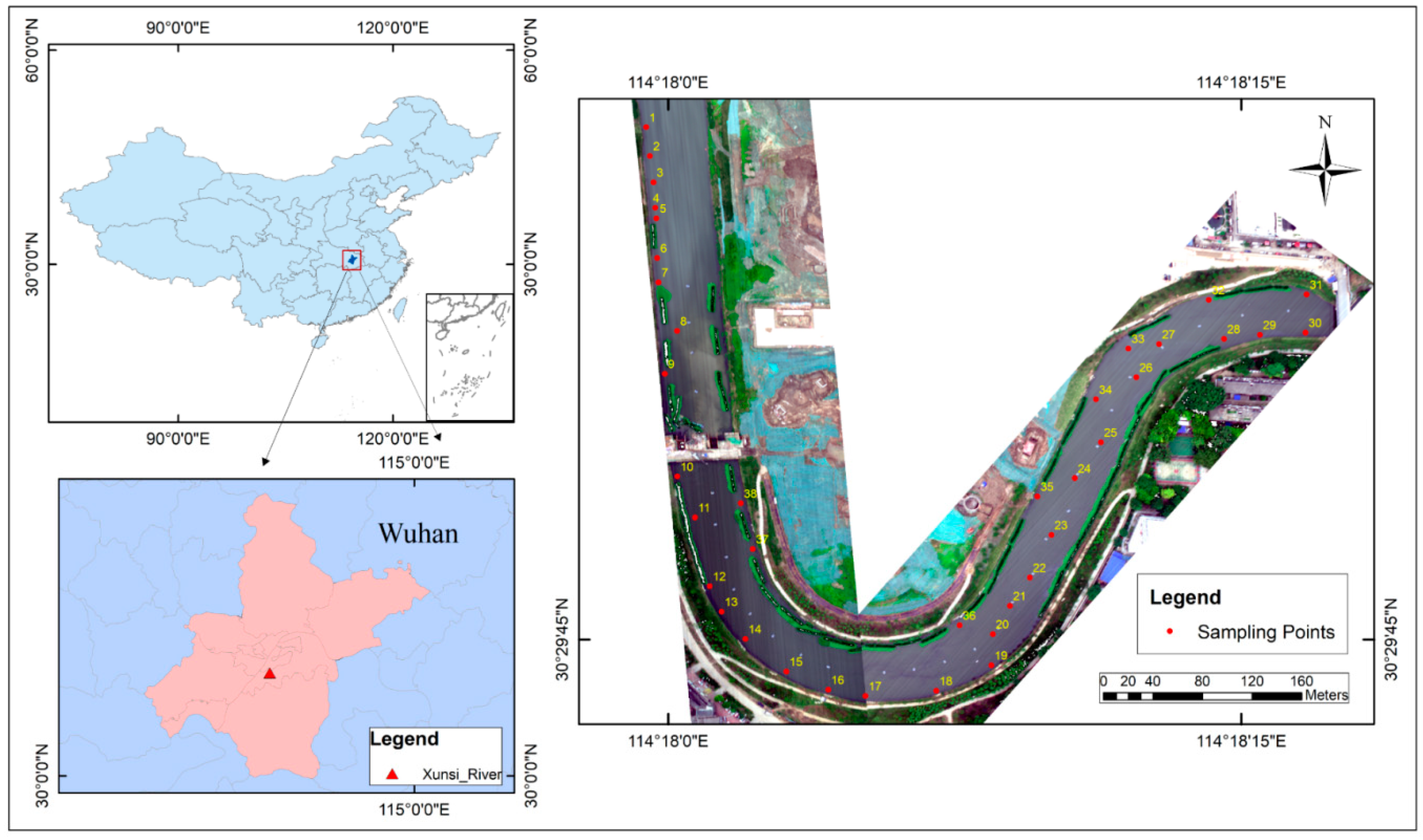
2.1. Study Area
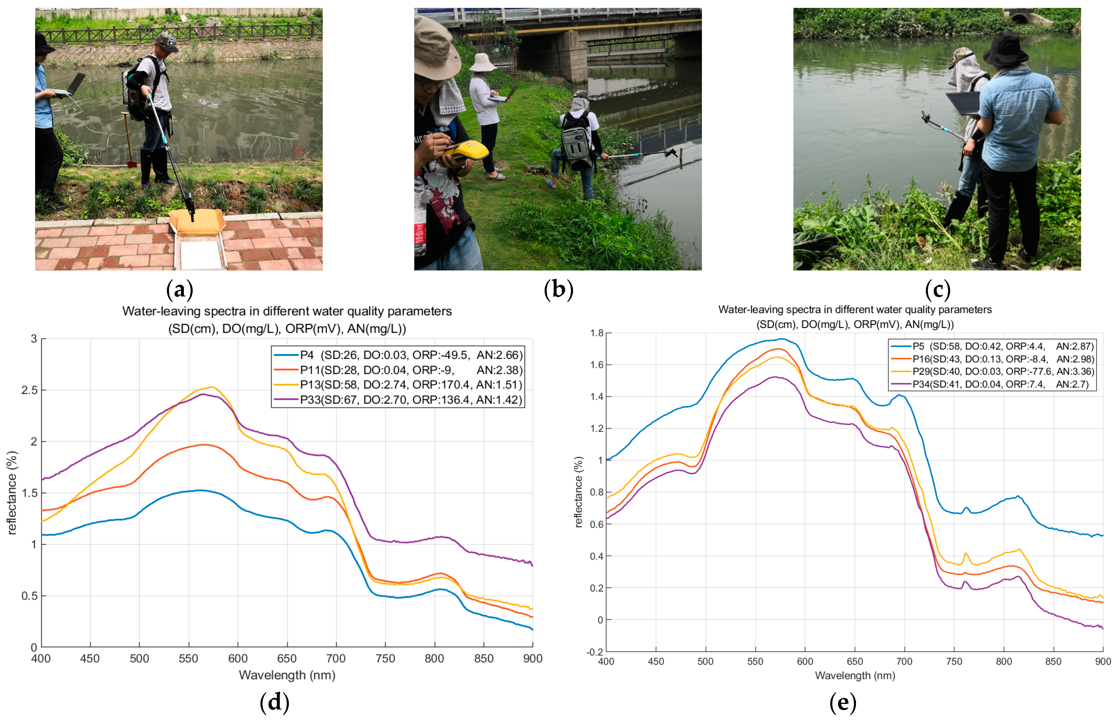
2.2. In Situ Data and Spectra Collection
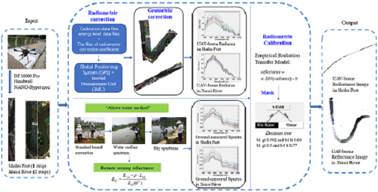
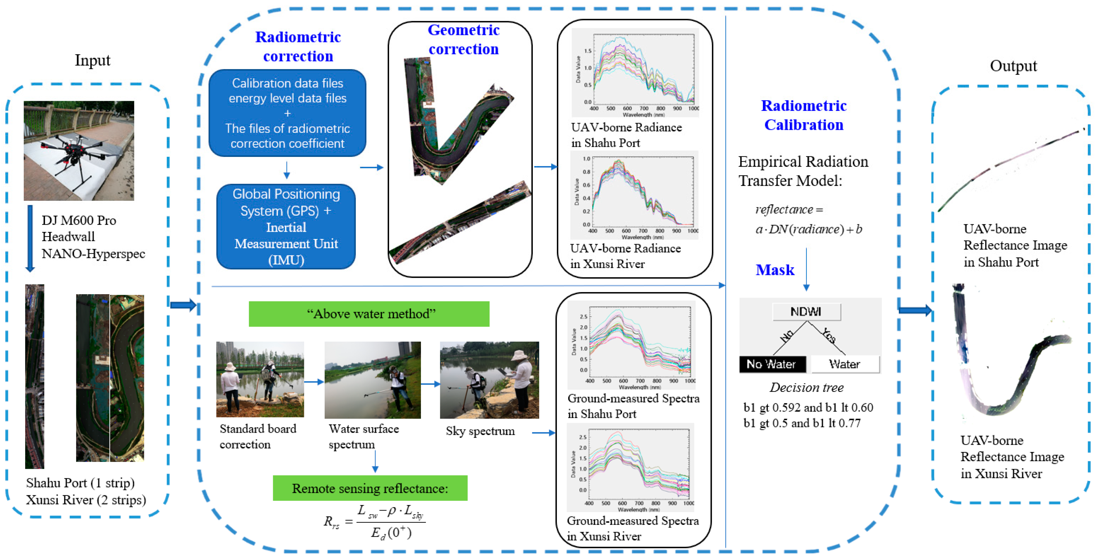
2.3. Airborne Hyperspectral Imagery and Preprocessing
- (1)
- The sensor radiation calibration converts the signal output by the sensor unit into actual radiance. In this study, the original image data were converted from DN value to radiance value by pixel, according to the model and the conversion parameters in the radiation correction document provided by the hyperspectral sensor manufacturer;
- (2)
- The UAV-borne Headwall Nano-Hyperspec hyperspectral sensor used in this study is a linear push-broom imaging sensor. Therefore, it is easily affected by shake during the flight, which can cause severe deformation of the obtained imagery. The UAV features a position and orientation system (POS) which integrates differential GPS technology and inertial measurement unit (IMU) technology. The POS can provide sensor position and attitude parameters to directly and quickly geolocate the images to the correct geographic location;
- (3)
- Due to the difference in illumination geometry and flight time between the two strips, this may cause other changes in the remote sensing images, in addition to the interference factors caused by water quality changes. Therefore, it was necessary to adjust the second strip with the first strip as a reference, and to then splice the two strips. The imagery was processed using ENVI, and the histogram was matched to the entire image;
- (4)
- The radiation calibration of hyperspectral imagery is commonly undertaken in the 6S atmospheric correction model and the MODTRAN model, but these models are only suitable for the situation where the atmospheric environment during the flight is relatively complicated and the flight height of the UAV is high (at the kilometer level). The flight areas of this study were located in urban areas, and the relative flight was only 200 m. Therefore, in the radiation calibration, we could ignore the complex atmospheric effects and only consider the linear relationship of the DN or radiance measured on board and the in-site reflectance [32,33,34]. Since the reflectivity of the standard board could not meet the experimental requirements, the linear relationship calibration of the UAV-borne radiance images was completed by the use of ground-measured spectra [35]. The number of ground-measured spectra used for the absolute radiation calibration in the two study areas was 29 and 23, respectively. The calibration program was written in IDL/ENVI, and the linear function fitted by the ground spectra and UAV spectra was applied to the radiation calibration of the UAV-borne images;
- (5)
- The UAV-borne images had a wavelength range of 400–1000 nm, covering the visible to near-infrared. Since the mid-infrared band which is usually used in the modified normalized difference water index (MNDWI) was not covered, we used a green (560 nm) and a near-infrared (830 nm) band for masking in this experiment [36], and the water area was extracted by a decision tree model. The normalized difference water index (NDWI) threshold in Shahu Port was [0.592, 0.6], and the threshold in Xunsi River was [0.5, 0.77].
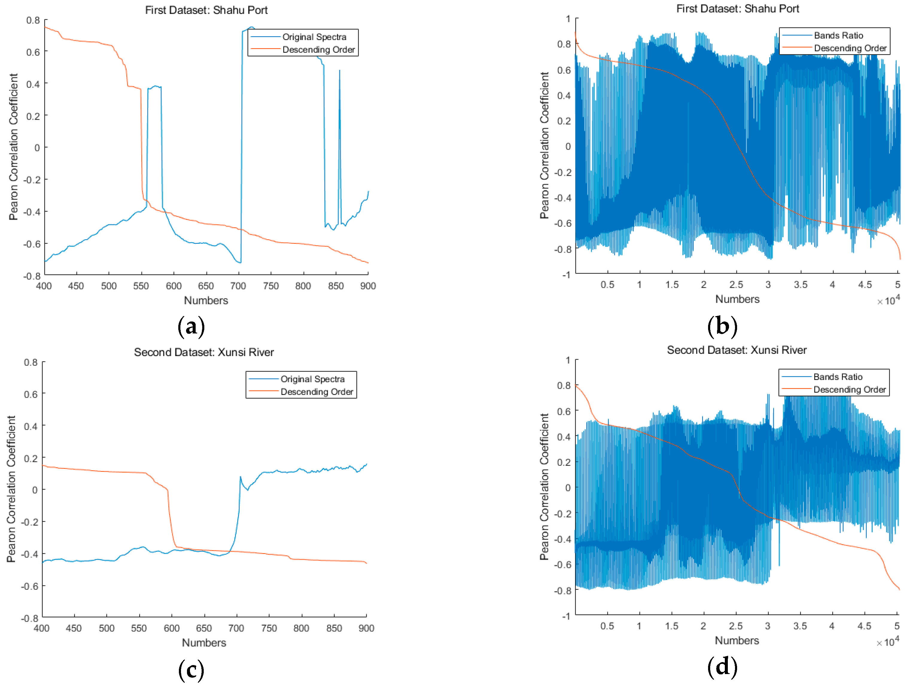
2.4. Spectral Data Preprocessing
2.5. Modeling Approaches
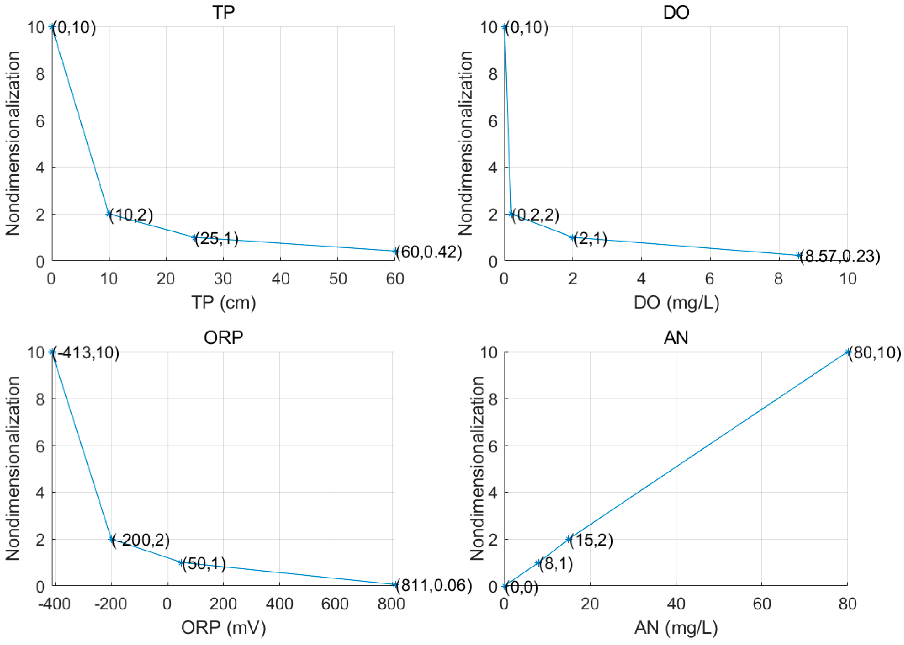
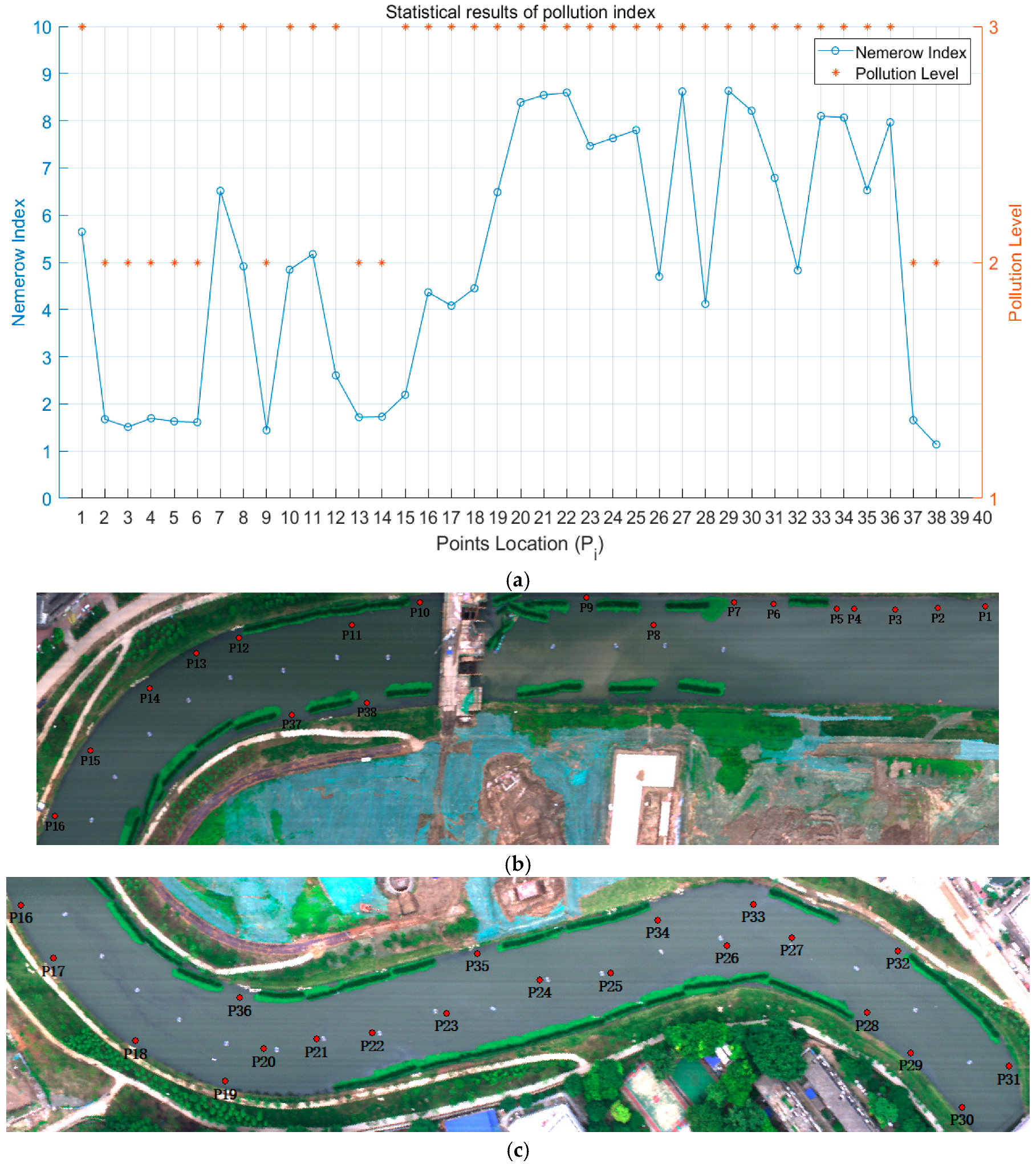
2.5.1. Nemerow Comprehensive Pollution Index
2.5.2. Gradient Boosting Decision Tree and Other Models
2.5.3. Statistical Analysis
3. Results and Discussion
3.1. Gradient Boosting Decision Tree
3.2. First Dataset: Shahu Port
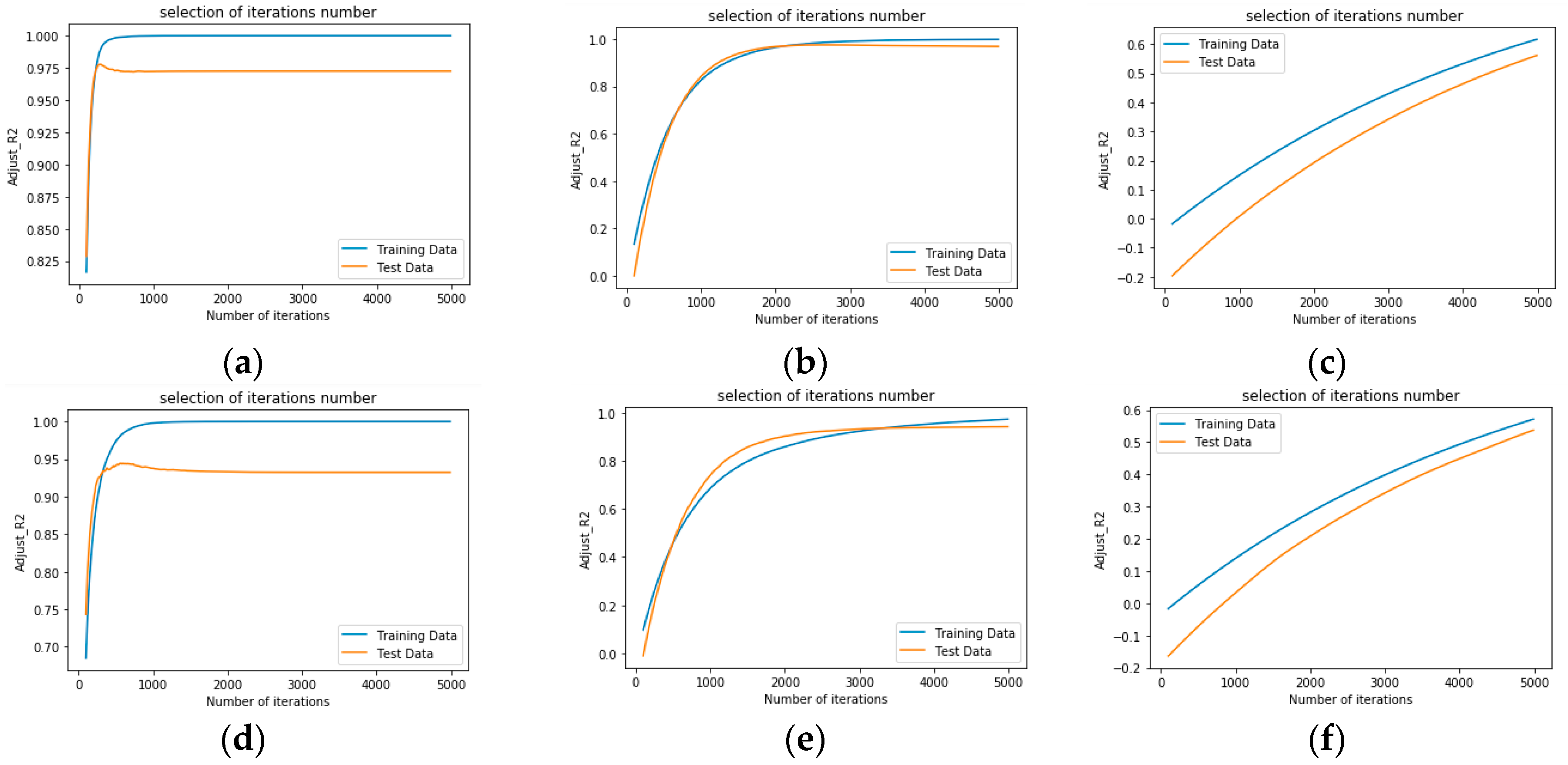
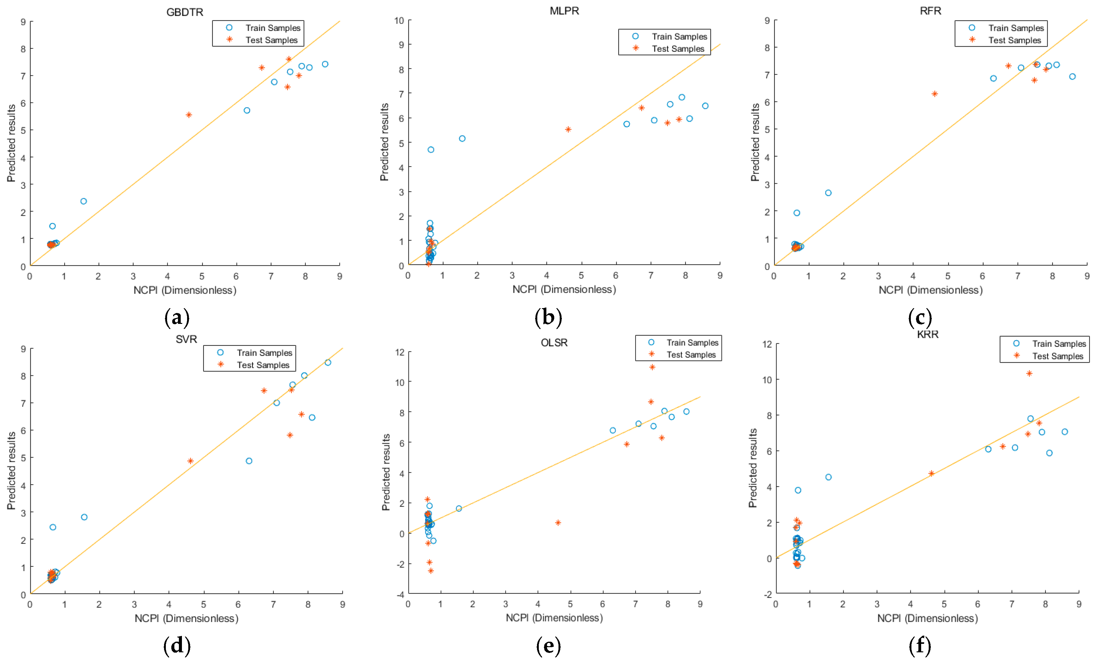
3.2.1. Model Optimization and Accuracy Evaluation
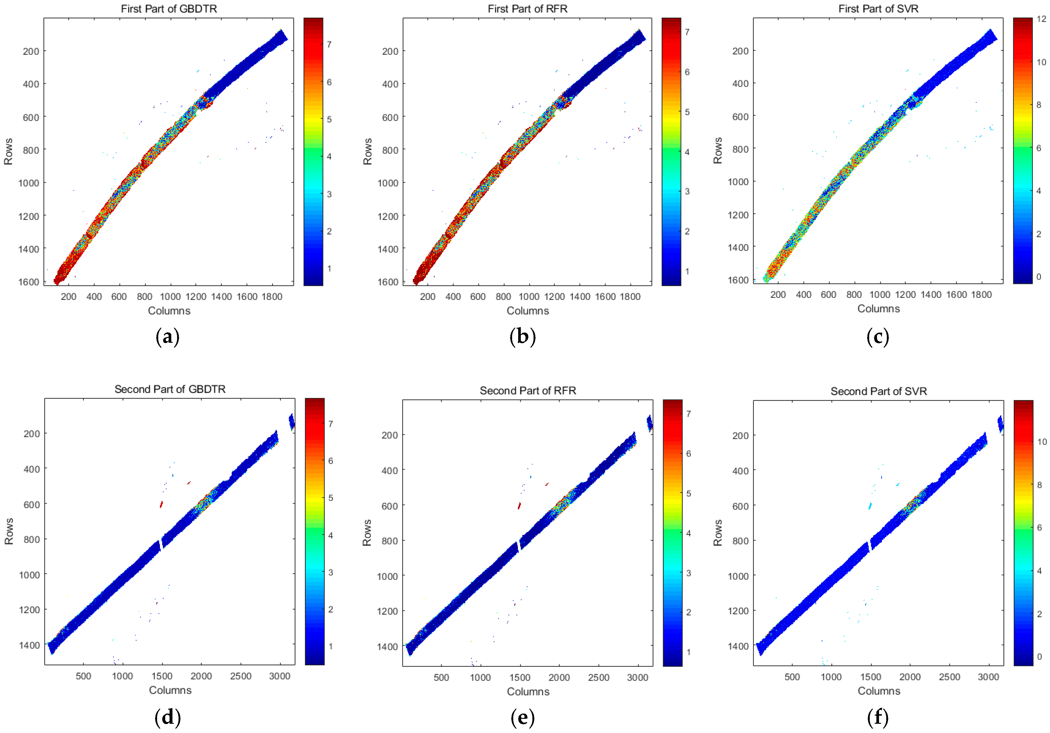
3.2.2. UAV-Borne Image Inversion Based on the Different Models
3.3. Second Dataset: Xunsi River
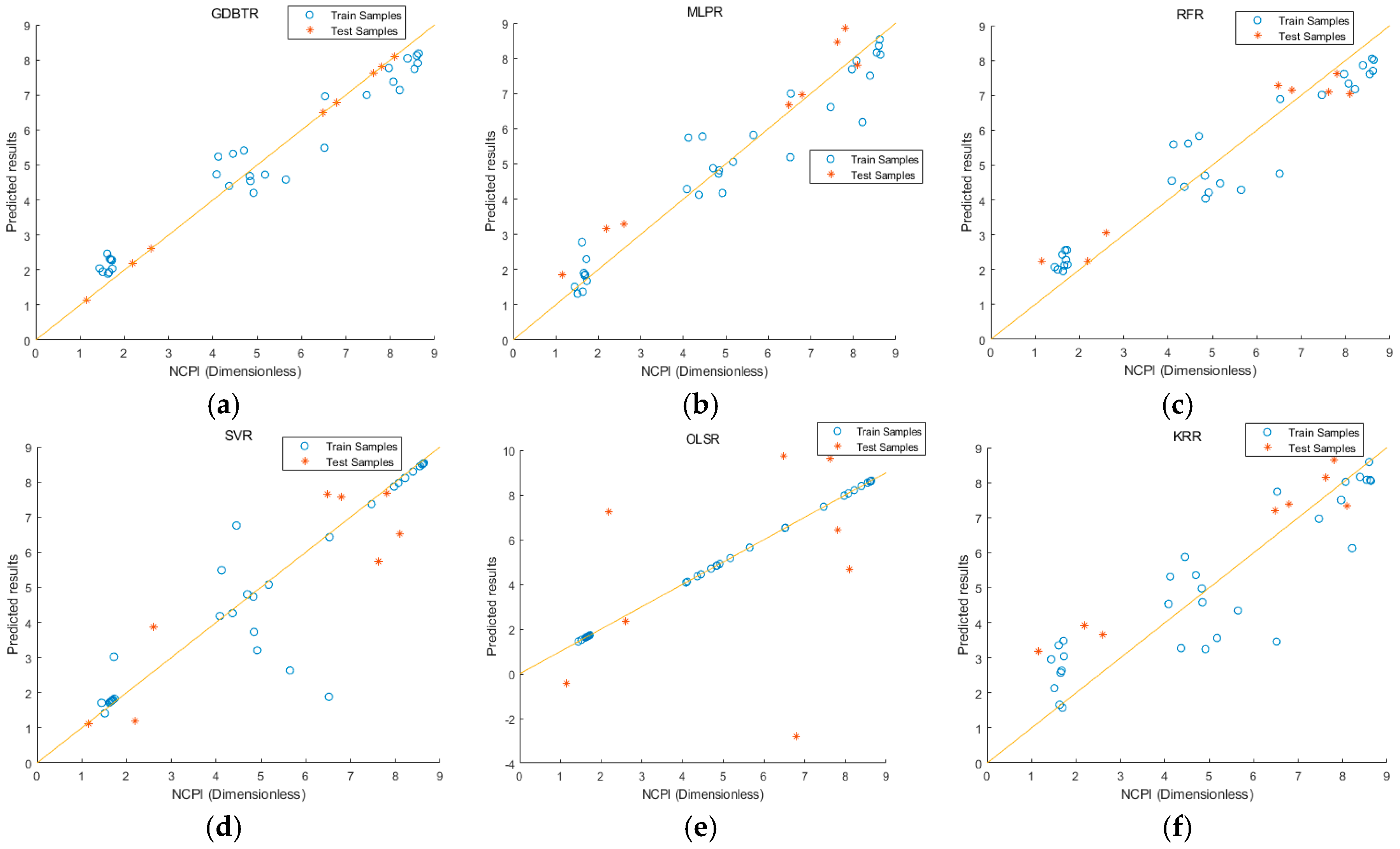
3.3.1. Model Optimization and Accuracy Evaluation
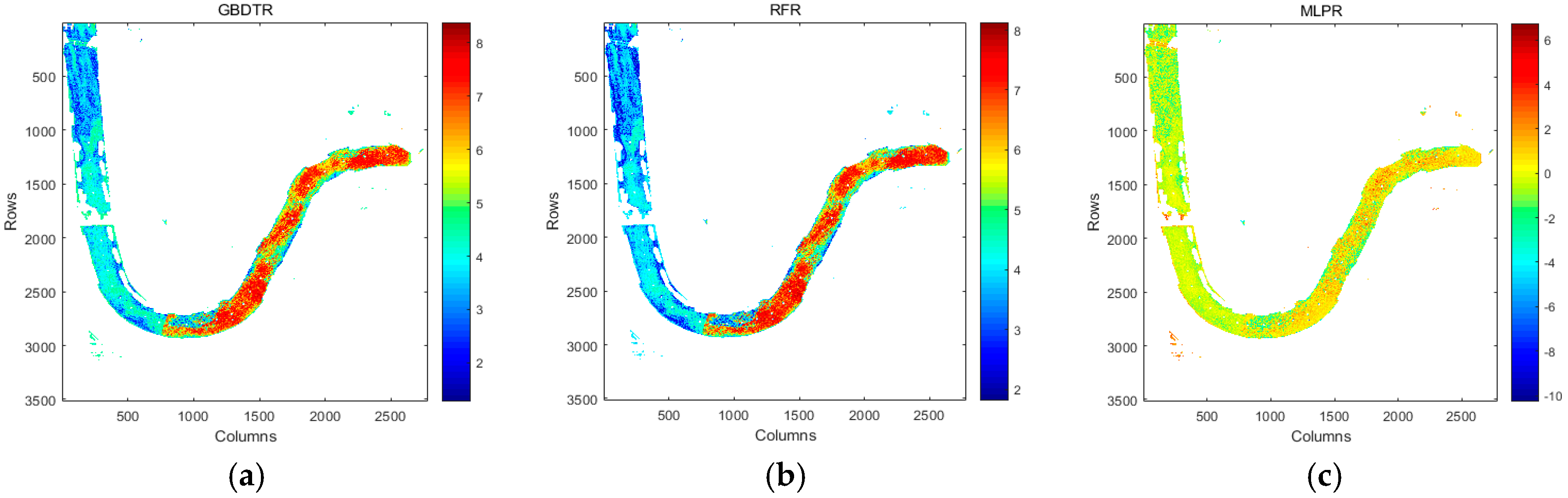
3.3.2. UAV-Borne Image Inversion Based on the Different Models
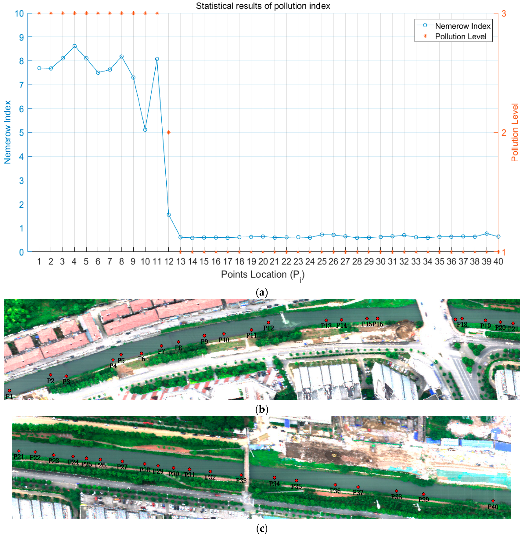
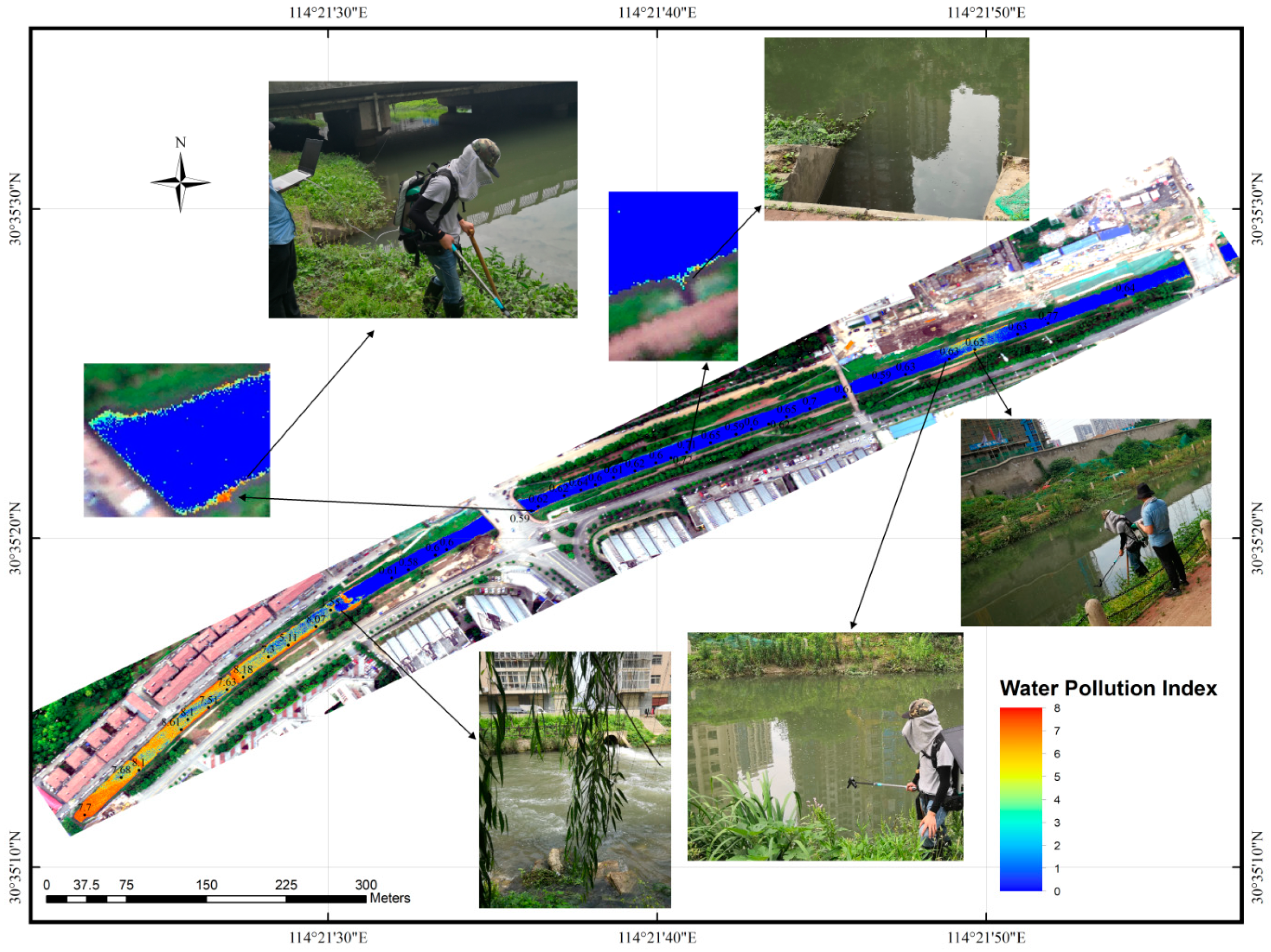
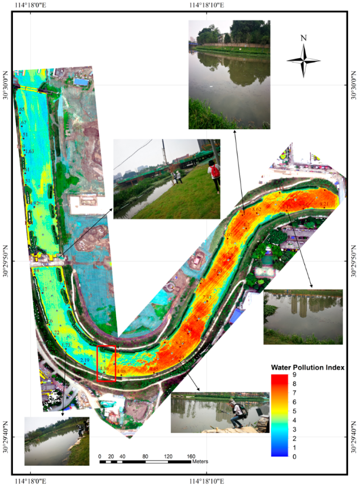
3.4. UAV-Borne Image Inversion Based on the Gradient Boosting Decision Tree Regression Model
4. Conclusions
Author Contributions
Funding
Acknowledgments
Conflicts of Interest
References
- Wang, J.; Liu, X.D.; Lu, J. Urban river pollution control and remediation. Procedia Environ. Sci. 2012, 13, 1856–1862. [Google Scholar] [CrossRef]
- He, D.F.; Chen, R.R.; Zhu, E.H.; Chen, N.; Yang, B.; Shi, H.H.; Huang, M.S. Toxicity bioassays for water from black-odor rivers in Wenzhou, China. Environ. Sci. Pollut. Res. 2015, 22, 1731–1741. [Google Scholar]
- Xue, W.; Tao, T.; Yang, J.; Wu, J.; Duan, S. Summary on ecological treatment of urban river. Sci. Soil Water Conserv. 2008, 6, 106–111. [Google Scholar]
- Diaz, R.J.; Rosenberg, R. Spreading dead zones and consequences for marine ecosystems. Science 2008, 321, 926–929. [Google Scholar] [CrossRef] [PubMed]
- Pucciarelli, S.; Buonanno, F.; Pellegrini, G.; Pozzi, S.; Ballarini, P.; Miceli, C. Biomonitoring of Lake Garda: Identification of ciliate species and symbiotic algae responsible for the “black-spot” bloom during the summer of 2004. Environ. Res. 2008, 107, 194–200. [Google Scholar] [CrossRef] [PubMed]
- Shen, Q.; Liu, C.; Zhou, Q.; Shang, J.; Zhang, L.; Fan, C. Effects of physical and chemical characteristics of surface sediments in the formation of shallow lake algae-induced black bloom. J. Environ. Sci. 2013, 25, 2353–2360. [Google Scholar] [CrossRef]
- Chen, G.; Luo, J.; Zhang, C.; Jiang, L.; Tian, L.; Guangping, C. Characteristics and influencing factors of spatial differentiation of urban black and odorous waters in China. Sustainability 2018, 10, 4747. [Google Scholar] [CrossRef]
- Alp, E.; Melching, C.S. Allocation of supplementary aeration stations in the Chicago waterway system for dissolved oxygen improvement. J. Environ. Manag. 2011, 92, 1577–1583. [Google Scholar] [CrossRef]
- Noblet, J.; Schweitzer, L.; Ibrahim, E.; Stolzenbach, K.D.; Zhou, L.; Suffet, I.H. Evaluation of a taste and odor incident on the Ohio River. Water Sci. Technol. 1999, 40, 185–193. [Google Scholar] [CrossRef]
- Peng, W.; Yisong, W.; Pingfang, Z.; Mei, L.; Jingya, S.; Fusheng, Z. Analysis of formation and mechanisms of black and smelly river water in island cities. Meteorol. Environ. Res. 2018, 9, 42–48. [Google Scholar]
- Romano, A.H.; Safferman, R.S. Studies on actinomycetes and their odors. J. Am. Water Work. Assoc. 1963, 55, 169–176. [Google Scholar] [CrossRef]
- Battin, T.J. Dissolved organic matter and its optical properties in a blackwater tributary of the upper Orinoco river, Venezuela. Org. Geochem. 1998, 28, 561–569. [Google Scholar] [CrossRef]
- Berthon, J.-F.; Zibordi, G. Optically black waters in the northern Baltic Sea. Geophys. Res. Lett. 2010, 37. [Google Scholar] [CrossRef]
- Peter, A.; Köster, O.; Schildknecht, A.; von Gunten, U. Occurrence of dissolved and particle-bound taste and odor compounds in Swiss lake waters. Water Res. 2009, 43, 2191–2200. [Google Scholar] [CrossRef] [PubMed]
- Salem, S.I.; Strand, M.H.; Higa, H.; Kim, H.; Kazuhiro, K.; Oki, K.; Oki, T.; Salem, S.I.; Strand, M.H.; Higa, H. Evaluation of MERIS chlorophyll-a retrieval processors in a complex turbid lake Kasumigaura over a 10-year mission. Remote Sens. 2017, 9, 1022. [Google Scholar] [CrossRef]
- Duan, H.; Ma, R.; Loiselle, S.A.; Shen, Q.; Yin, H.; Zhang, Y. Optical characterization of black water blooms in eutrophic waters. Sci. Total Environ. 2014, 482–483, 174–183. [Google Scholar] [CrossRef]
- Shuang, W.; Qiao, W.; Yun-Mei, L.I.; Li, Z.; Heng, L.; Lei, S.H.; Ding, X.L.; Song, M. Remote sensing identification of urban black-odor water bodies based on high-resolution images: A case study in Nanjing. Environ. Sci. 2018, 39, 57–67. [Google Scholar]
- Lei, Z.; Bing, Z.; Junsheng, L.; Qian, S.; Fangfang, Z.; Ganlin, W. A study on retrieval algorithm of black water aggregation in Taihu Lake based on HJ-1 satellite images. In IOP Conference Series: Earth and Environmental Science; IOP Publishing: Bristol, UK, 2014; Volume 17. [Google Scholar]
- Ministry of Housing and Urban-Rural Development of China. The Guideline for Urban Black and Odorous Water Treatment; Ministry of Housing and Urban-Rural Development of China: Beijing, China, 2015. (In Chinese)
- Nemerow, N.L. (Ed.) Stream, Lake, Estuary, and Ocean Pollution; Van Nostrand Reinhold Publishing Co.: New York, NY, USA, 1991; pp. 0–472. [Google Scholar]
- Brady, J.P.; Ayoko, G.A.; Martens, W.N.; Goonetilleke, A. Development of a hybrid pollution index for heavy metals in marine and estuarine sediments. Environ. Monit. Assess. 2015, 187, 306. [Google Scholar] [CrossRef]
- Liu, X.; Heilig, G.K.; Chen, J.; Heino, M. Interactions between economic growth and environmental quality in Shenzhen, China’s first special economic zone. Ecol. Econ. 2007, 62, 559–570. [Google Scholar] [CrossRef]
- Arroyo-Mora, J.; Kalacska, M.; Inamdar, D.; Soffer, R.; Lucanus, O.; Gorman, J.; Naprstek, T.; Schaaf, E.; Ifimov, G.; Elmer, K.; et al. Implementation of a UAV–hyperspectral pushbroom imager for ecological monitoring. Drones 2019, 3, 12. [Google Scholar] [CrossRef]
- Houborg, R.; Soegaard, H.; Boegh, E. Combining vegetation index and model inversion methods for the extraction of key vegetation biophysical parameters using Terra and Aqua MODIS reflectance data. Remote Sens. Environ. 2007, 106, 39–58. [Google Scholar] [CrossRef]
- Mueller, J.L.; Fargion, G.S.; McClain, C.R.; Mueller, J.L.; Morel, A.; Frouin, R.; Davis, C.; Arnone, R.; Carder, K.; Steward, R.G.; et al. Ocean Optics Protocols for Satellite Ocean Color Sensor Validation, Revision 4, Volume III: Radiometric Measurements and Data Analysis Protocols; NASA Goddard Space Flight Center: Greenbelt, MD, USA, 2003. [Google Scholar]
- Niroumand-Jadidi, M.; Pahlevan, N.; Vitti, A. Mapping substrate types and compositions in shallow streams. Remote Sens. 2019, 11, 262. [Google Scholar] [CrossRef]
- Lee, Z.; Carder, K.L.; Steward, R.G.; Peacock, T.G.; Davis, C.O.; Mueller, J.L. Remote sensing reflectance and inherent optical properties of oceanic waters derived from above-water measurements. In Ocean Optics XIII; International Society for Optics and Photonics: Bellingham, WA, USA, 1997; Volume 2963, pp. 160–166. [Google Scholar]
- Mobley, C.D. Estimation of the remote-sensing reflectance from above-surface measurements. Appl. Opt. 1999, 38, 7442–7455. [Google Scholar] [CrossRef] [PubMed]
- Rhea, W.J.; Davis, C.O. A comparison of the SeaWiFS chlorophyll and CZCS pigment algorithms using optical data from the 1992 JGOFS Equatorial Pacific Time Series. Deep Sea Res. Part II Top. Stud. Oceanogr. 1997, 44, 1907–1925. [Google Scholar] [CrossRef]
- Watanabe, F.; Alcântara, E.; Rodrigues, T.; Imai, N.; Barbosa, C.; Rotta, L. Estimation of chlorophyll-a concentration and the trophic state of the Barra Bonita hydroelectric reservoir using OLI/Landsat-8 images. Int. J. Environ. Res. Public Health 2015, 12, 10391–10417. [Google Scholar] [CrossRef] [PubMed]
- Zhong, Y.; Wang, X.; Xu, Y.; Wang, S.; Jia, T.; Hu, X.; Zhao, J.; Wei, L.; Zhang, L. Mini-UAV-borne hyperspectral remote sensing: From observation and processing to applications. IEEE Geosci. Remote Sens. Mag. 2018, 6, 46–62. [Google Scholar] [CrossRef]
- Ben-Dor, E.; Kindel, B.; Goetz, A.F.H. Quality assessment of several methods to recover surface reflectance using synthetic imaging spectroscopy data. Remote Sens. Environ. 2004, 90, 389–404. [Google Scholar] [CrossRef]
- Smith, G.; Milton, E. The use of the empirical line method to calibrate remotely sensed data to reflectance. Int. J. Remote Sens. 1999, 20, 2653–2662. [Google Scholar] [CrossRef]
- Malenovský, Z.; Lucieer, A.; King, D.H.; Turnbull, J.D.; Robinson, S.A. Unmanned aircraft system advances health mapping of fragile polar vegetation. Methods Ecol. Evol. 2017, 8, 1842–1857. [Google Scholar] [CrossRef]
- Niroumand-Jadidi, M.; Vitti, A.; Lyzenga, D.R. Multiple Optimal Depth Predictors Analysis (MODPA) for river bathymetry: Findings from spectroradiometry, simulations, and satellite imagery. Remote Sens. Environ. 2018, 218, 132–147. [Google Scholar] [CrossRef]
- Niroumand-Jadidi, M.; Vitti, A. Reconstruction of river boundaries at sub-pixel resolution: Estimation and spatial allocation of water fractions. ISPRS Int. J. Geo Inf. 2017, 6, 383. [Google Scholar] [CrossRef]
- Pulliainen, J.; Kallio, K.; Eloheimo, K.; Koponen, S.; Servomaa, H.; Hannonen, T.; Tauriainen, S.; Hallikainen, M. A semi-operative approach to lake water quality retrieval from remote sensing data. Sci. Total Environ. 2001, 268, 79–93. [Google Scholar] [CrossRef]
- Legleiter, C.J.; Roberts, D.A.; Lawrence, R.L. Spectrally based remote sensing of river bathymetry. Earth Surf. Process. Landf. 2009, 34, 1039–1059. [Google Scholar] [CrossRef]
- Niroumand-Jadidi, M.; Vitti, A. optimal band ratio analysis of worldview-3 imagery for bathymetry of shallow rivers (case study: Sarca River, Italy). Int. Arch. Photogramm. Remote Sens. Spat. Inf. Sci. 2016, XLI-B8, 361–364. [Google Scholar] [CrossRef]
- Legleiter, C.J.; Stegman, T.K.; Overstreet, B.T. Spectrally based mapping of riverbed composition. Geomorphology 2016, 264, 61–79. [Google Scholar] [CrossRef]
- Bekhet, H.A.; Yasmin, T. Exploring EKC, trends of growth patterns and air pollutants concentration level in Malaysia: A nemerow index approach. In IOP Conference Series: Earth and Environmental Science; IOP Publishing: Bristol, UK, 2013; Volume 16. [Google Scholar]
- Guan, Y.; Shao, C.; Ju, M. Heavy metal contamination assessment and partition for industrial and mining gathering areas. IJERPH 2014, 11, 7286–7303. [Google Scholar] [CrossRef] [PubMed]
- Bi, S.; Yang, Y.; Xu, C.; Zhang, Y.; Zhang, X.; Zhang, X. Distribution of heavy metals and environmental assessment of surface sediment of typical estuaries in eastern China. Mar. Pollut. Bull. 2017, 121, 357–366. [Google Scholar] [CrossRef]
- Friedman, J.H. Greedy function approximation: A gradient boosting machine. Ann. Stat. 2001, 29, 1189–1232. [Google Scholar] [CrossRef]
- Wang, H.; Meng, Y.; Yin, P.; Hua, J. A model-driven method for quality reviews detection: An ensemble model of feature selection. In Proceedings of the Wuhan International Conference on E-Business, Wuhan, China, 27–29 May 2016; p. 2. [Google Scholar]
- Yuan, X.; Abouelenien, M. A multi-class boosting method for learning from imbalanced data. IJGCRSIS 2015, 4, 13–29. [Google Scholar] [CrossRef]
- Wei, L.; Yuan, Z.; Yu, M.; Huang, C.; Cao, L. Estimation of arsenic content in soil based on laboratory and field reflectance spectroscopy. Sensors 2019, 19, 3904. [Google Scholar] [CrossRef]
- Zou, Y.; Ding, Y.; Tang, J.; Guo, F.; Peng, L. FKRR-MVSF: A fuzzy kernel ridge regression model for identifying DNA-binding proteins by multi-view sequence features via Chou’s five-step rule. Int. J. Mol. Sci. 2019, 20, 4175. [Google Scholar] [CrossRef] [PubMed]
- Ebrahimi, M.; Mohammadi-Dehcheshmeh, M.; Ebrahimie, E.; Petrovski, K.R. Comprehensive analysis of machine learning models for prediction of sub-clinical mastitis: Deep learning and gradient-boosted trees outperform other models. Comput. Biol. Med. 2019, 114, 103456. [Google Scholar] [CrossRef] [PubMed]
- Huang, Z.; Yi, K. Communication-efficient weighted sampling and quantile summary for GBDT. arXiv 2019, arXiv:1909.07633. [Google Scholar]
- Wei, Z.; Meng, Y.; Zhang, W.; Peng, J.; Meng, L. Downscaling SMAP soil moisture estimation with gradient boosting decision tree regression over the Tibetan Plateau. Remote Sens. Environ. 2019, 225, 30–44. [Google Scholar] [CrossRef]
- Hafeez, S.; Wong, M.; Ho, H.; Nazeer, M.; Nichol, J.; Abbas, S.; Tang, D.; Lee, K.; Pun, L. Comparison of machine learning algorithms for retrieval of water quality indicators in case-II waters: A case study of Hong Kong. Remote Sens. 2019, 11, 617. [Google Scholar] [CrossRef]
- Wang, Z.; Kawamura, K.; Sakuno, Y.; Fan, X.; Gong, Z.; Lim, J. Retrieval of chlorophyll-a and total suspended solids using iterative stepwise elimination partial least squares (ISE-PLS) regression based on field hyperspectral measurements in irrigation ponds in Higashihiroshima, Japan. Remote Sens. 2017, 9, 264. [Google Scholar] [CrossRef]
- Shen, X.; Cao, L.; Chen, D.; Sun, Y.; Wang, G.; Ruan, H. Prediction of forest structural parameters using airborne full-waveform LiDAR and hyperspectral data in subtropical forests. Remote Sens. 2018, 10, 1729. [Google Scholar] [CrossRef]


| Characteristic Indicator | Mild | Severe |
|---|---|---|
| SD (cm) | 25–10 | <10 |
| DO (mg/L) | 0.2–2.0 | <0.2 |
| ORP (mV) | −200–50 | <−200 |
| AN (mg/L) | 8.0–15 | >15 |
| Modeling Method | Training Data | Test Data | ||||
|---|---|---|---|---|---|---|
| Adjusted_R2 | RMSE | MAPE | Adjusted_R2 | RMSE | MAPE | |
| GBDTR | 0.978 | 0.41 | 24.69% | 0.974 | 0.48 | 18.96% |
| MLPR | 0.823 | 1.18 | 53.78% | 0.809 | 1.31 | 44.25% |
| RFR | 0.968 | 0.50 | 17.11% | 0.962 | 0.58 | 9.41% |
| SVR | 0.956 | 0.59 | 22.11% | 0.954 | 0.64 | 13.72% |
| OLSR | 0.970 | 0.48 | 43.69% | 0.506 | 2.11 | 145.11% |
| KRR | 0.850 | 1.09 | 76.94% | 0.850 | 1.16 | 98.36% |
| Modeling Method | Computation Time (s) | Min Value | Max Value |
|---|---|---|---|
| — | — | 0.59 | 8.61 |
| GBDTR | 178 | 0.48 | 7.71 |
| RFR | 4010 | 0.62 | 7.35 |
| SVR | 43 | −0.45 | 12.04 |
| Modeling Method | Training Data | Test Data | ||||
|---|---|---|---|---|---|---|
| Adjusted_R2 | RMSE | MAPE | Adjusted_R2 | RMSE | MAPE | |
| GBDTR | 0.938 | 0.64 | 16.59% | 0.936 | 0.63 | 16.97% |
| MLPR | 0.924 | 0.71 | 12.59% | 0.921 | 0.70 | 20.92% |
| RFR | 0.900 | 0.82 | 20.34% | 0.926 | 0.67 | 19.63% |
| SVR | 0.781 | 1.21 | 14.25% | 0.783 | 1.16 | 21.56% |
| OLSR | 1.000 | 6.46e−13 | 1.71e−11% | 0 | 4.30 | 81.84% |
| KRR | 0.794 | 1.17 | 29.61% | 0.781 | 1.16 | 43.29% |
| Modeling Method | Computing Time (s) | Max Value | Min Value |
|---|---|---|---|
| — | — | 8.62 | 1.14 |
| GBDTR | 785 | 8.38 | 1.27 |
| RFR | 27316 | 8.12 | 1.81 |
| MLPR | 174 | 6.75 | −10.27 |
© 2019 by the authors. Licensee MDPI, Basel, Switzerland. This article is an open access article distributed under the terms and conditions of the Creative Commons Attribution (CC BY) license (http://creativecommons.org/licenses/by/4.0/).
Share and Cite
Wei, L.; Huang, C.; Wang, Z.; Wang, Z.; Zhou, X.; Cao, L. Monitoring of Urban Black-Odor Water Based on Nemerow Index and Gradient Boosting Decision Tree Regression Using UAV-Borne Hyperspectral Imagery. Remote Sens. 2019, 11, 2402. https://doi.org/10.3390/rs11202402
Wei L, Huang C, Wang Z, Wang Z, Zhou X, Cao L. Monitoring of Urban Black-Odor Water Based on Nemerow Index and Gradient Boosting Decision Tree Regression Using UAV-Borne Hyperspectral Imagery. Remote Sensing. 2019; 11(20):2402. https://doi.org/10.3390/rs11202402
Chicago/Turabian StyleWei, Lifei, Can Huang, Zhengxiang Wang, Zhou Wang, Xiaocheng Zhou, and Liqin Cao. 2019. "Monitoring of Urban Black-Odor Water Based on Nemerow Index and Gradient Boosting Decision Tree Regression Using UAV-Borne Hyperspectral Imagery" Remote Sensing 11, no. 20: 2402. https://doi.org/10.3390/rs11202402
APA StyleWei, L., Huang, C., Wang, Z., Wang, Z., Zhou, X., & Cao, L. (2019). Monitoring of Urban Black-Odor Water Based on Nemerow Index and Gradient Boosting Decision Tree Regression Using UAV-Borne Hyperspectral Imagery. Remote Sensing, 11(20), 2402. https://doi.org/10.3390/rs11202402