Article

Detection of Geothermal Potential Zones Using Remote Sensing Techniques

by
David Lago González
and
Pablo Rodríguez-Gonzálvez
*
Department of Mining Technology, Topography and Structures, Universidad de León, 24401 Ponferrada, Spain
*
Author to whom correspondence should be addressed.
Remote Sens. 2019, 11(20), 2403; https://doi.org/10.3390/rs11202403
Submission received: 23 August 2019 / Revised: 12 October 2019 / Accepted: 15 October 2019 / Published: 16 October 2019

Abstract

:
The transition towards a new sustainable energy model—replacing fossil fuels with renewable sources—presents a multidisciplinary challenge. One of the major decarbonization issues is the question of to optimize energy transport networks for renewable energy sources. Within the range of renewable energies, the location and evaluation of geothermal energy is associated with costly processes, such as drilling, which limit its use. Therefore, the present research is aimed at applying different geomatic techniques for the detection of geothermal resources. The workflow is based on free/open access geospatial data. More specifically, remote sensing information (Sentinel-2A and Advanced Spaceborne Thermal Emission and Reflection Radiometer (ASTER)), geological information, distribution of gravimetric anomalies, and geographic information systems have been used to detect areas of shallow geothermal potential in the northwest of the province of Orense, Spain. Due to the variety of parameters involved, and the complexity of the classification, a random forest classifier was employed, since this algorithm works well with large sets of data and can be used with categorical and numerical data. The results obtained allowed identifying a susceptible area to be operated on with a geothermal potential of 80 W·m−1 or higher.

Graphical Abstract

1. Introduction

Fossil fuels (coal, petroleum, and natural gas) encompassed 81% of the total primary energy supply in 2016 [1]. These energy sources are characterized by their limited reserves and for producing greenhouse gases (GHG), which cause, as consequences, the increase of the average temperature and extreme changes in the climate, among others. Climate change stabilization requires us to impose limitations on GHG emissions from fossil fuel combustion, thus, to try to minimize the effects of climate change, governments of different countries have accepted and ratified agreements, including an energy transition from fossil fuels to renewable energies [2].
One of the least widespread renewable energies in the world is geothermal [3], which uses the Earth’s internal heat to generate heat in buildings and to generate energy in geothermal plants. Geothermal energy is defined as the energy stored in the form of heat beneath the surface of solid Earth [4]. Among the different types of geothermal energy: very low, low, high, and very high enthalpy, the present research is focused in low or very-low enthalpy types, also known as shallow types [5]. This energy is characterized by being partially renewable, having high availability, reducing GHG emissions [6], and producing less waste than other energy sources.
The detection of areas with geothermal potential was initially carried out by means of perforations to measure the temperature in the subsoil. Despite the fact that this method is accurate, it relies on the estimation of the geothermal reservoir parameters (thickness, porosity, permeability, and temperature) to estimate the geothermal potential [7]. Another factor to consider are the significant costs for the drilling operations. For this reason, different researchers have tried to develop methodologies to reduce costs in the search for these areas, taking into great consideration the use of remote sensing as a means to prioritize zones of potential geothermal energy [8,9], due to the availability of free satellite imagery and its cost-effective ratio for the geothermal exploration of large areas. One approach that involves remote sensing is the search for areas of rocks altered by hydrological action using images from one or more sensors, since they are indicative of thermal fluids being discharged along faults [10]. Surface thermal properties are an indicator of geothermal resources, which can be measured by the use of images from thermal sensors [11,12]. Additionally, temperatures can also be obtained using multispectral imagery [13] acquiring land surface temperature (LST) values.
Among the geomatic techniques, geographic information systems (GIS) offer a whole new dimensionality by combining the remote sensing data with other geographic information sources as in [14], in which gravimetric anomalies, thermal images, and the location of geological faults were employed. Among the available GIS techniques, the use of random forest classifiers stands out, since they allow the ability to extract information from categorical and numerical variables. As a result, they support the decision-taking process without significant computational requirements. These algorithms are popular among the scientific community due to its ease of use and being able to be applied in multiple fields as in the case of [15], in which they were used to obtain a model of the demand of electricity. Another transversal example is the application to the solar energy field [16], in which authors employed classifiers such as random forest, extra trees, and support vector regression to carry out a comparison among them and to evaluate which hour range is more useful for a solar thermal system.
The present article proposes a combination of geomatic techniques along with different free/open sources to delimit potential geothermal areas potential in a simple and non-invasive way. The rest of the paper is organized as follows: Section 2 describes the methodology of the developed approach and the materials employed. Prediction results are presented in Section 3, along with the validation of the classification. Discussion is detailed in Section 4, whereas concluding remarks and future research directions are presented at the end of the paper in Section 5.

2. Materials and Methods

2.1. Methodology

The present work is organized as follows: Firstly, a land cover map of the study area was created to isolate the areas susceptible of geothermal exploitation. Secondly, the LST, geological faults and Bouguer anomalies were generated using free/open data sources. The masked areas were trained against the ground truth of geothermal potential using a random forest algorithm. Finally, a GIS analysis was employed to locate the undiscovered areas and quantify the efficiency of the process. Next, a summary of the workflow is shown (Figure 1).
The geographic data processing was carried out using three software. Firstly, QGIS (Quantum Geographic Information System) with the Semi-Automatic Classification (SPC) plugin [17] and the GDAL (Geospatial Data Abstraction Library) georeferencer plugin [18], were used, respectively, for the download and pre-processing of the Sentinel-2A images, and for the re-georeferencing of the geological map. Secondly, ENVI 5.0 (Exelis Visual Information Solutions) was employed for the classifications of the Sentinel-2A images and the processing of the thermal images. And, finally ArcGIS 10.4.1, which was used to perform auxiliary tasks (e.g., image clipping or conversion to different image formats), digitize raster maps and for the final classification.

2.1.1. Land Cover Creation

Through the use of the Sentinel-2A images, it is possible to create a mask in order to exclude non-relevant areas, which encompasses vegetation, water zones, and infrastructures. These last three classes were not to be taken into account in the classification and subsequent GIS analysis.
Though the use of QGIS’ plugin Semi-Automatic Classification [17] Sentinel 2 Level 1C images can be downloaded for further processing and conversion at level 2A. The Semi-Automatic Classification plugin allows the ability to apply the dark object substation (DOS) to the images before converting to radiances and then reflectances. This method, according to [19], is based on the basic assumption that within the image some pixels are in full shadow and their satellite radiances are due to atmospheric scattering (path radiance). This assumption is combined with the fact that very few surface targets on Earth are absolute blacks, so a minimum reflectance of one percent better than zero percent is assumed. The path radiance (Lp) resulted from the interaction of the electromagnetic radiance with the atmospheric components is obtained by [20]:
L P = L m i n L D 01 % ,
where Lmin is the radiance that corresponds to a digital count value for which the sum of all pixels with digital counts lower or equal to the 0.01% of all pixels from the image considered; whereas LD01% is the dark object radiance, assuming it has a reflectance value of 0.01. In the case of the Sentinel 2 images, these are converted to radiances before applying the DOS correction. The dark object radiance is given by [17,20]:
L D 01 % = 0.01 [ ( E S U N λ cos ( θ S ) T Z ) + E d o w n ] T v π d 2 ,
where TV and TZ are the atmospheric transmittance along the atmospheric trajectory from the ground to the sensor, Edown is the downward irradiance due to the solar flux dispersed in the atmosphere, and ϑS is the solar zenith angle. The mean solar exo-atmospheric irradiances (ESUNλ) values were obtained from [17]. Since there are several DOS techniques, the simplest one, DOS1, was employed, where the values for the aforementioned coefficients are: TV = 1, TZ = 1, and Edown = 0 [21]. From these corrected radiance values, surface reflectance can be calculated by the following equation:
ρ = π ( L λ L p ) d 2 [ T v ( ( E S U N λ cos ( θ S ) T Z ) + E d o w n ) ]
where Lλ is the spectral radiance at the sensor’s aperture (at-satellite radiance), and d is the Earth–Sun distance in astronomical units.
Using ENVI 5.0., two indexes are created for each one of the satellite images to allow detecting vegetation and infrastructures zones with great ease. The first index is the normalized difference vegetation index (NDVI) [22]. This index is used to determine the amount of vegetation in an area. Its value varies from −1 to +1. The NDVI is calculated using the following equation with the near-infrared (NIR) and red (R) bands.
N D V I = N I R R N I R + R
The second index employed is the normalized difference building index (NDBI) [23], which is used to determine built areas. The NDBI is calculated using the following equation according to a short wave infrared band (SWIR).
N D B I = N I R S W I R N I R + S W I R
By the use of a vector file with the administrative limits of the analyzed region, a new file that delimits the study area was created, to crop the images. After the pre-processing of the images, the classification of the principal soil surfaces was carried out: vegetation, infrastructures, water, pasture, bare soil, shrubland, and outdoor. To carry out the classification, a maximum likelihood algorithm was used. This classifier assumes that the data sample follows a normal distribution to assign the probability that a pixel belongs to a predeterminate class. It offers robustness of calculation [24]. The chosen calculation coefficients were a scale factor of 1 and 4000 and a probability threshold of 0% in both cases. The scale factor was used to convert whole scale reflectance data into floating point values.
Once classified, the images were validated using both a visual check, to eliminate those combinations that exhibit significant problems when classifying, and a validation by a set of validation points on the image to calculate the confusion matrices. Additionally, the Cohen’s kappa coefficient, overall accuracy, user accuracy, and producer accuracy were computed. For the two last parameters (user and producer accuracy) the confidence intervals at 95% confidence interval were computed using the adjusted Wald method [25,26]. This method is chosen since provides the best coverage when the sample size is less than 150 [27].
The combination of parameters that provided the better results were applied to the rest of the images.

2.1.2. Land Surface Temperature (LST) Map

The variation of temperature with depth is called a geothermal gradient, and raises with increasing depth in the Earth’s crust. The thermal energy generated and stored in the Earth’s core, mantle, and crust is transferred towards the surface, mostly by conduction. This conductive heat flow makes the temperature rise with increasing depth in the crust on average 25–30 °C/km [28]. With the aforementioned average thermal gradient, a 1 km geothermal drill in a dry rock formation would have a bottom temperature near 40 °C [28].
The first step to generate the soil temperature image is to calibrate the satellite images to obtain radiance images. In order to perform this step, it is necessary convert the digital levels (DL) to the spectral radiance at the sensor’s aperture (Lλ) in radiance units (W·m−2·sr−1·μm−1) according to Equation (6). The parameters of the linear calibration (gain and offset) can be obtained from the image’s metadata.
L λ = G a i n D L + O f f s e t
The LST map is carried out using ENVI software [29,30]. This software has implemented several algorithms to calculate the emissivity, but in the present research the emissivity alpha residual method was used [31]. This algorithm uses an approximation of the Wien law of the Plank function, so it offers results with a 1%–2% error for temperatures of 300 K (27 °C) at a wavelength of 10 μm [32]. The obtention of the LST is based on the law of Planck, which relates the energy emitted by a blackbody (emissivity = 1) with its temperature. However, while most of the natural elements are non-black bodies (0 < ελ < 1), it is necessary to modify Planck’s law according to its spectral emissivity (ελ) according to the following equation:
L ( λ , T ) = ε ( λ ) L B B ( λ , T ) = ε ( λ ) c 1 λ 5 π ( e c 2 λ T 1 ) ,
where L(λ,T) is the spectral radiance of the natural object, LBB the blackbody radiance, λ the wavelength and c1 and c2 the first and second radiation constants. Based on Equation (7), if the radiance values have been corrected for atmospheric effects and the emissivity of the surface is known, the temperature value (T) can be obtained as follows:
T = c 2 λ ln ( ε 1 c 1 π λ 5 L ) + 1 .
The above expression is based on the assumption that the surface cover behaves like a perfect Lambertian reflector. Please note that the result obtained from Equation (8) is expressed in Kelvin, so a transformation to Celsius degrees is required.

2.1.3. Geological Map

To add the geological map as a layer for the GIS analysis, it is necessary to digitize the national geological map. The first step is to reduce the number of informational classes present in the legend, which includes more than fifty different elements. This large number of elements will not improve the final analysis, in addition to complicating the digitization process and decision making. So, a reclassification of these classes into new ones was performed. The new classes were created according to the rock formation process [33]. A total of six informational classes were created, which are described below in Table 1 [34].
With the new classes defined, a digitization process was applied over the geological map. If necessary, a geo-referencing operation could be applied to ensure the correct fit of all individual map sheets. Once the informational classes (Table 1) were digitized, a topological revision was carried out to verify that the classes do not overlap each other or with themselves.

2.1.4. Geological Fault Map

By the use of ArcGIS, the faults are digitalized using the geological map (see previous subsection). They are split into two classes: one for known faults, and another one for supposed faults (Figure 2),
Once the known and supposed faults are digitized as line features, the influence zones or buffers were computed using ArcGIS. The employed criterion for the selection of the distance thresholds is that proposed by Li et al., 2017 [14], in which seven influence zones separated from each other by a distance of one kilometer are created. Since the size of the study area of [14] encompasses 10,956 km2, an area greater than the present study case (2236.37 km2), it is necessary to scale the distance between the influence zones. Therefore, for the present research, the distance interval is reduced to 250 m. After the buffer creation, it could appear that overlap among the influence zones of the known and supposed faults in certain areas occurred. So, a priority was given to the areas of known fault over the supposed ones. Finally, the different vector files generated were grouped into a single vector file that was later converted into raster for the final GIS analysis.

2.1.5. Bouguer Anomalies Map

Since satellite images only report the superficial behavior, additional data was employed, in this case related to the subsoil density distribution, by means of gravimetric anomaly data. More specifically, gravimetric anomalies were added to the classification, since they can be used to identify subsurface geological structures of interest. Gravimetric anomalies have an important role in geodesy and geophysics [35]. In geodesy they are used to define the figure of the Earth. The geophysical approach aims to highlight local anomalies, which are used to deduce variations in the mass and density of the geological surface, minimizing regional gravimetric anomalies, such as the presence of mountains. In this particular project, we focused on the geophysical approach, since Bouguer anomalies can be applied to the search for aquifers [36]. For more details related to the gravimetric anomalies, please refer to [37,38].

2.1.6. GIS Analysis

The multilayer analysis was carried out by a random forest decision classifier because of the complexity in decision-making and the large number of parameters to be taken into account. Random forest is an ensemble classifier that produces many classification and regression-like trees where each tree is generated from different bootstrapped samples of training data [39]. This algorithm has shown that one can obtain more accurate results than other classification techniques, such as maximum likelihood, when using data obtained from different sources [40]. The first step for the GIS analysis is the selection of the training zones. They are selected from the ground-truth information (Section 2.2.4.).
The training of the random forest in ArcGIS was carried out using a multilayer image, in which each of the layer corresponds to the maps generated (Section 2.1.1, Section 2.1.2, Section 2.1.3, Section 2.1.4 and Section 2.1.5). Finally, the mask of the area of interest was used to proceed with the final analysis of the occupied surface for each of the classes with geothermal potential, avoiding the non-interest areas. These areas correspond to surfaces classified as water, vegetation, or infrastructure.

2.2. Materials

Next, the materials employed are described. They encompass satellite imagery, gravimetric anomalies, geological maps, and resources from spatial data infrastructures.

2.2.1. Satellite Imagery

Due to the research requirements, there were different sources of satellite images considered due to the different spectral information provided.
Firstly, the Sentinel-2A sensor, which is part of the Copernicus program of the European Space Agency, is characterized by having a high-resolution camera with bands covering the visible, near infrared (NIR), and middle wave infrared (SWIR) regions, with spatial resolutions of 10, 20, or 60 m and with a radiometric resolution of 12 bits, and that allows the ability to obtain images with a revisit time of 10 days [41]. This sensor was employed to generate a land cover map (Section 2.1.1.). By means of this land cover it was possible to exclude areas where the exploitation of geothermal energy was not possible, such as water or infrastructure areas.
Secondly, the other type of images that were used were those of NASA’s Advanced Spaceborne Thermal Emission Reflection Radiometer (ASTER) sensor [42], which allows the ability to obtain images from the same place every 16 days, with information in 14 bands that cover the visible-infrared (VNIR), SWIR, and thermal infrared (TIR), with spatial resolutions of 15, 30, and 90 m respectively. The thermal images of the ASTER sensor were used to make a map of land surface temperatures, of high spatial resolution (90 m), to seek the correspondence between soil and subsoil temperatures (Section 2.1.2.).

2.2.2. Geological Map

The geological model was obtained from the Spanish National Geological Map (MAGNA) [43], at a scale of 1:50,000. The MAGNA was used to create a map of rocks and minerals, since certain types of rocks and minerals are associated with geothermal activity (Section 2.1.3.). Due to the huge amount of types of rocks in the study area, all the available informational classes were simplified into six classes, to reduce the digitation and processing time. Once the vector file corresponding with the study area was loaded, a non-total correspondence with the administrative limits was detected. This indicates a georeferencing problem of the MAGNA map, therefore, all the individual map sheets were re-georeferenced. To carry it out, the first step was to combine all the individual map sheets into a single raster file, since this eases the subsequent process, and allows the ability to apply the corrections in a more homogeneous way. The georeferencing was carried out with the GDAL plugin [18] available in QGIS.
Another use of the MAGNA was to obtain information about geological faults located in the study area. If the rocks surrounding magma chambers are permeable or fractured, and there is underground water circulation, the latter captures the heat of the rocks, being able to ascend to the surface through cracks or faults, leading to the formation of water hot springs, geysers, fumaroles, and mud volcanoes [44]. So, faults are geological structures favorably correlated to the existence of geothermal reservoirs [45,46].
The MAGNA geological series classifies the faults in two groups, known and supposed faults. The faults were digitized using the re-georeferenced geological map; so, two vector files were created with information about them (Section 2.1.4.).

2.2.3. Gravimetric Anomalies

The data were obtained from the International Gravimetric Bureau [47]. The original format of 2′ × 2′ grid in geographical coordinates requires the reprojection to the coordinate reference system of the study case (in the present case European Terrestrial Reference System 1989 (ETRS89) Universal Transverse Mercator (UTM) 29N). Next, a resampling operation (nearest neighbor) was applied to homogenize the pixel size in relation to the temperature data obtained from the ASTER images, which have a spatial resolution of 90 m.

2.2.4. Ground-Truth Information

The ground truth for the classification was obtained by the International Renewable Energy Agency (IRENA) [48]. More specifically, the Spain map of geothermal potential distributed by the IRENA’s spatial data infrastructure [49]. This map, compilated from the Spanish Institute for the Diversification and Saving of Energy (IDAE) [50], shows the accessible, available, and total potential of geothermal resources for Spain. This map was used to obtain training areas to carry out the classification using a random forest classifier. The index for defining the geothermal potential is the estimated linear heat extraction/injection capability of the ground, expressed in W·m−1. The training areas were selected from the Web Map Service (WMS) of the International Renewable Energy Agency [49]. The distribution of the training areas on the WMS are shown in Figure 3.

3. Results

Next, the description of the study case, data employed, and the experimental results and their interpretation are drawn.

3.1. Study Case

The study area is located in the province of Ourense, in the autonomous community of Galicia, Spain. Specifically, in the northwest area of the province of Ourense, as can be seen in Figure 4. The province of Ourense is characterized by great orographic contrasts, with an altitudinal range between 60 and 2124 m. Among the mountains, there are a multitude of rivers, including the Sil and the Miño, which crosses the study area diagonally.
In Galicia, in general, it is possible to find zones of low to medium enthalpy between 200 and 1500 m [51]. The suitability of this area for the application of the present methodology is due, in part, to the presence of several thermal sources that were already known in Celtic and Roman times. As for example, the Ourense city was built around the Burgas’ springs of thermal water. In addition, there are other areas with geothermal potential in the towns of Celanova and Baños de Molgas.

Data

For the Sentinel-2, three images were downloaded from the Copernicus image server [52] with a 1C processing degree. The images were from the 17/06/2017 and 24/06/2017. The other satellite images employed were the ASTER. In total, four of daytime images were downloaded from Earthdata [53] were needed for the dates of 07/06 and 23/06 of 2017. The Bouguer anomaly data were obtained from the International Gravimetric Bureau (BGI) [47] in a grid format of 2′ × 2′. The geological data were obtained from the geological map of Spain (MAGNA); more specifically the sheets 153, 154, 186, 187, 188, 224, 225, 226, 262, 263, and 264 were needed to cover the complete study area.

3.2. Classification Validation

The first validation stage of the surface covers was a visual check, to dismiss the combination of algorithms and coefficients that provided non-coherent results, as for example, the classification of infrastructure areas. The maximum likelihood (ML) classification shows no significant difference among the different coefficient tested (scale factor), so, only the ML classification for a scale factor of 4000 was validated.
Through the confusion matrix (Table 2) it was possible to verify that the classification accuracy is high, as stated by an overall accuracy higher than 90% (up to 94.7%), and a kappa coefficient higher than 0.88 (up to 0.94). Although the high accuracy values obtained by the three classifications, due to the limitations of the approach, water zones, in which clouds were reflected, could not be classified correctly, and were assigned to the infrastructure class.
The validated classifier was applied to the satellite images to generate the land cover mosaic (Figure 5). An overlap priority was given to the image with the higher kappa coefficient.

3.3. Results

Next, the different layers that will be used in the GIS analysis are described in Figure 6, Figure 7, Figure 8 and Figure 9. The LST map in Celsius degrees (Figure 6) was obtained according to the methodology described in Section 2.1.2. Additionally, a cloud mask was created, since these zones do not contain valid soil temperature values. On the map it can be seen that the higher temperature zones correspond mostly to industrial or urban areas, while the lower temperature zones mostly correspond to the cloud areas, covered by the cloud mask.
The geological map (Figure 7) was created according the procedure described in Section 2.1.3. For the MAGNA re-georeferencing a total, thirty-six points were employed and distributed as homogeneously as possible for an optimal calculation and reprojection. The three-sigma criterion was applied to discard possible outliers [54].
Using the MAGNA data source, the fault (known and supposed) of the study area were digitized. Using the approached proposed in [14], the influences zones were computed with a distance interval of 250 m (Section 2.1.4.). The resulting layer is shown in Figure 8.
The last layer for the GIS analysis was the gravimetric anomalies map (Bouguer anomalies) as stated in Section 2.1.5. The resampled raster map, cropped for the study area extension, is shown in Figure 9. The low spatial resolution of the data source (grid of 2′ × 2′) is a significant constraint of the present layer.
Once the five layers were computed and combined into a single raster file, the GIS analysis was carried out using a random forest classifier. The first step involves the classifier training using the IRENA map [49]. A total of 569 training polygons were distributed in the study area (Figure 3) for the four classes of the geothermal potential provided by IRENA, as stated in Table 3. The parameters of the RF classification are a depth = 8 and number of trees = 100. For the assessment of the RF, k-fold cross-validation classification is employed, which split the training data into k equal-sized partitions [55]. The classifier was trained using k-1 folds, and the error was computed by checking the obtained classifier with the remaining fold. As a result, the classifier’s estimated error was the average value of the errors committed in each fold. For the study case, k was set to 10. The result of the final classification is shown in Figure 10.
The classification results are evaluated by means of the overall accuracy, Cohen’s Kappa index, and the receiving operating characteristic (ROC) curve area. The area under the ROC curve (AUC) provides a comparison between the predicted and actual instance values in a classification by measuring the precision and the recall [56]. The RF classification for the cross-validation achieved a Kappa index of 88.4%, an overall accuracy of 94.0% and an AUC equal to 98.7%. Please note that the last values correspond to the weighted averaged since the present classification employs a multi-class model [57].

4. Discussion

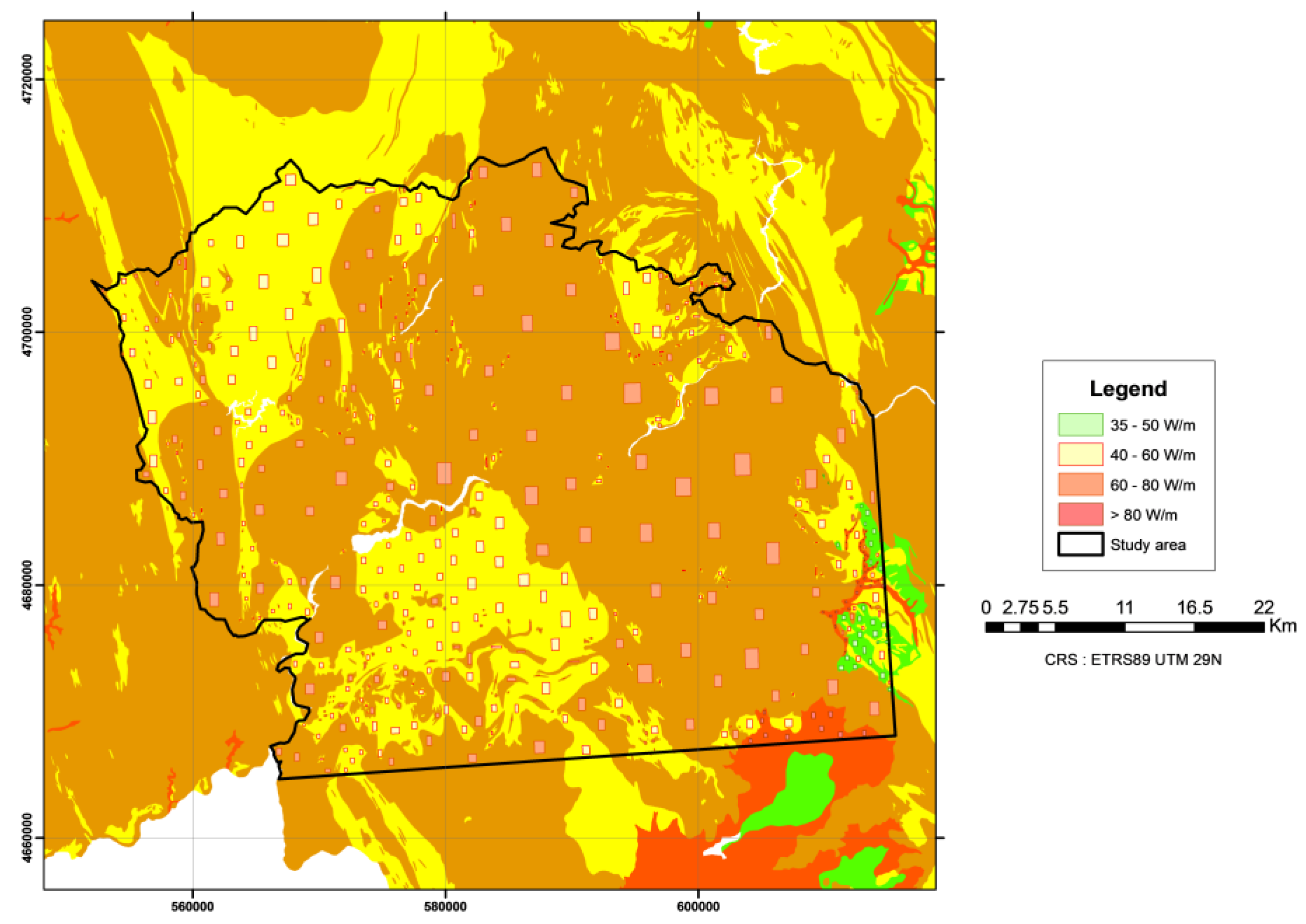
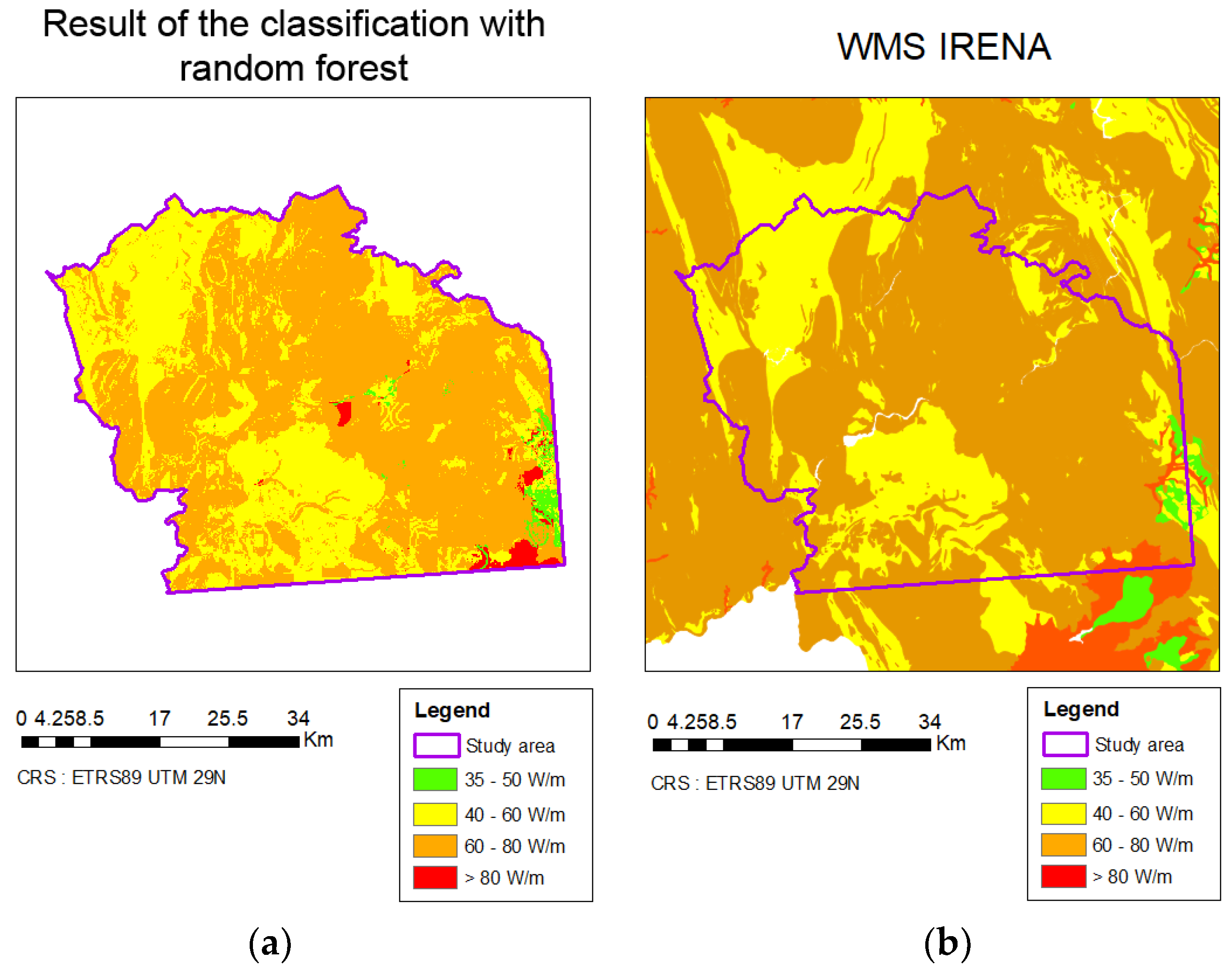
The result of the classification, as can be seen in Figure 11a, shows that areas with potential greater than 80 W·m−1 (highlighted in red) are found mainly in the southeast and east of the study area. Potential zones between 35 and 50 W·m−1, as expected, are located near the potential area, greater than 80 W·m−1, located in the east, in addition to a small area located near the center of the study area. The surface of each geothermal class is summed up in Table 4.
As can be seen in Figure 11b, there are a large number of common areas between the results obtained from the random forest classification and the IRENA map. Besides, it can be seen that the map obtained from the proposed classifier, the area related to a geothermal potential of 40–60 W·m−1 is larger than the stated by ground truth, which categorizes as 60–80 W·m
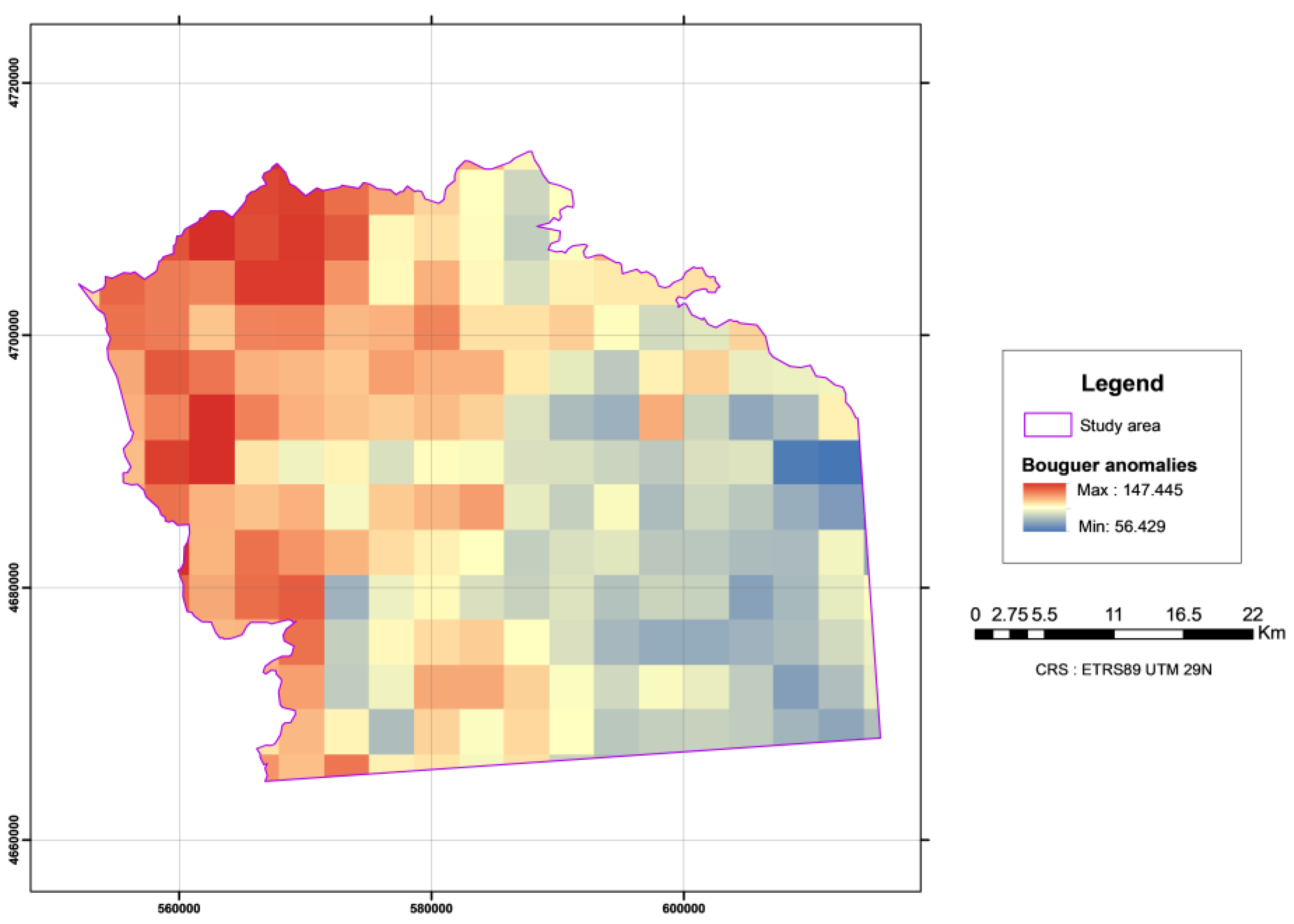
−1. Comparing this area with the Bouguer gravimetric anomalies map we can notice that the area of potential greater than 80 W·m−1 is located where the gravimetric anomalies are at its lowest, meaning that there is a relationship between them, as it was described in several works like [14,58,59].
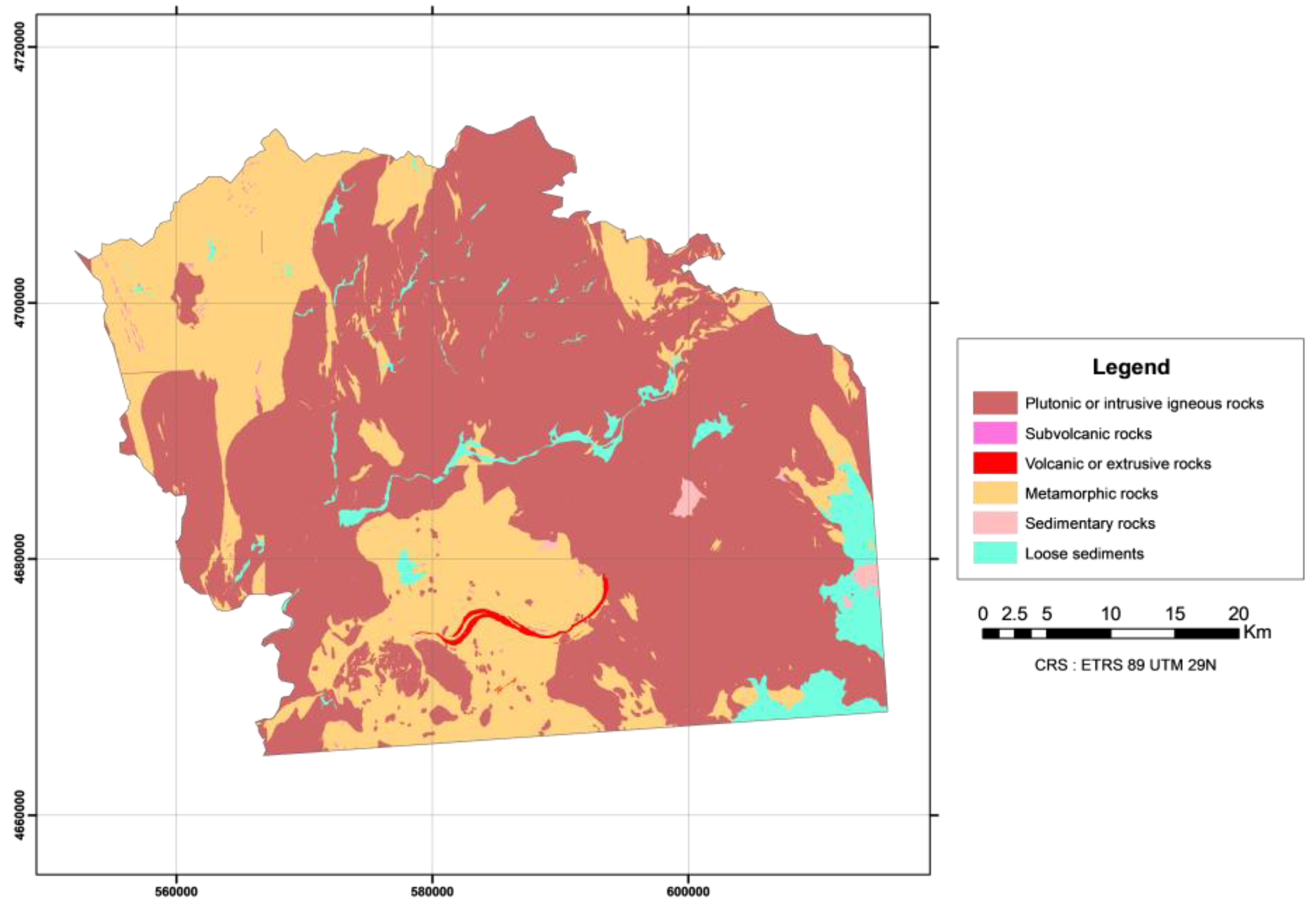
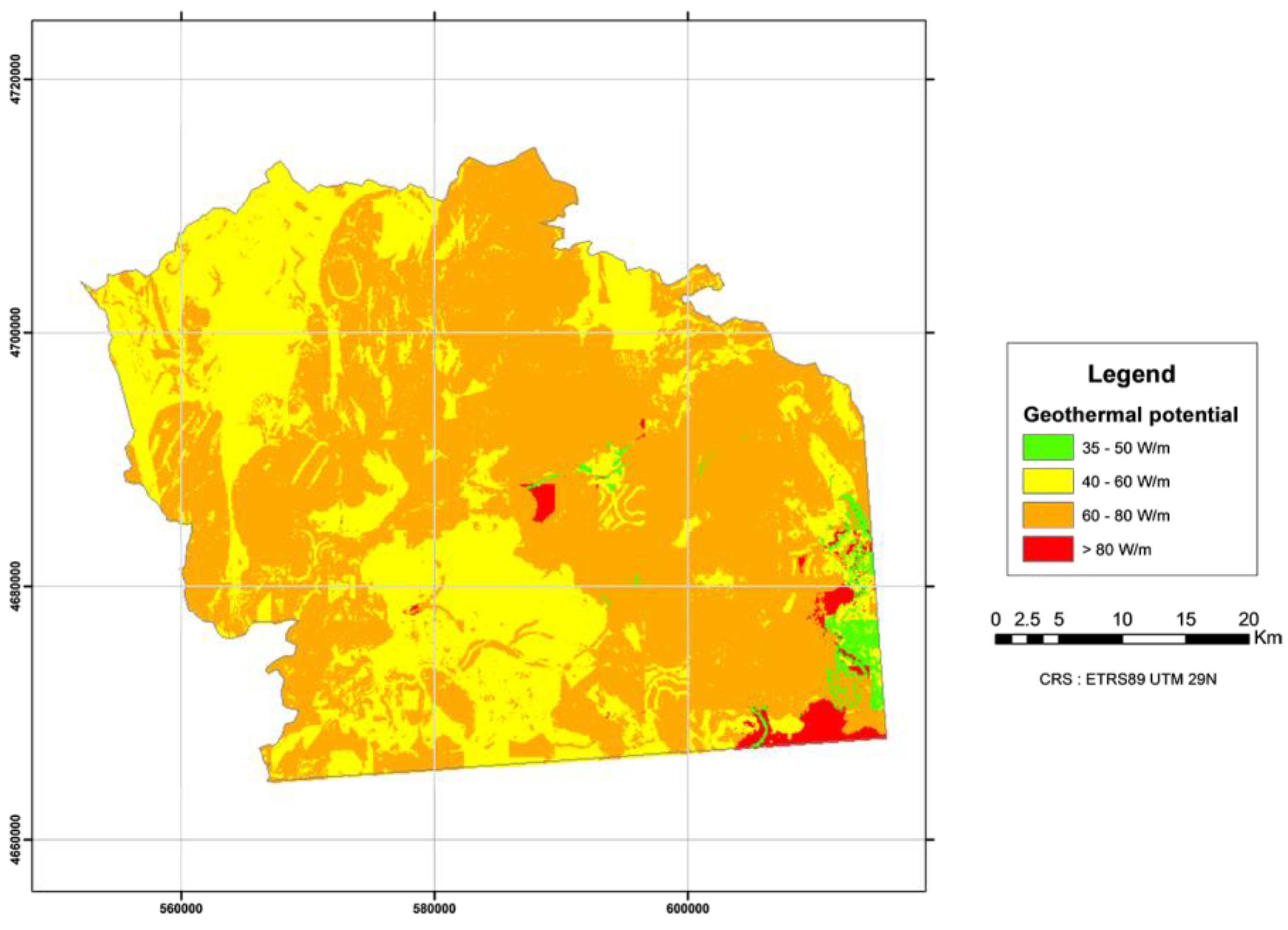
Paying attention to the geological map (Figure 7) and the geothermal potential map (Figure 10) there is a clear resemblance, as some areas look similar in both maps. For example, the area of potential greater than 80 W·m−1 located in the bottom east of the study area occupies the same area in the geological map as the loose sediments. Another example that stands out more is the case of the area of potential between 60 and 80 W·m−1, which occupies the same area as the plutonic or intrusive igneous rocks. This relationship between some types of rocks and sediments is not unfamiliar as some other researchers have noticed this relationship before [10,12].
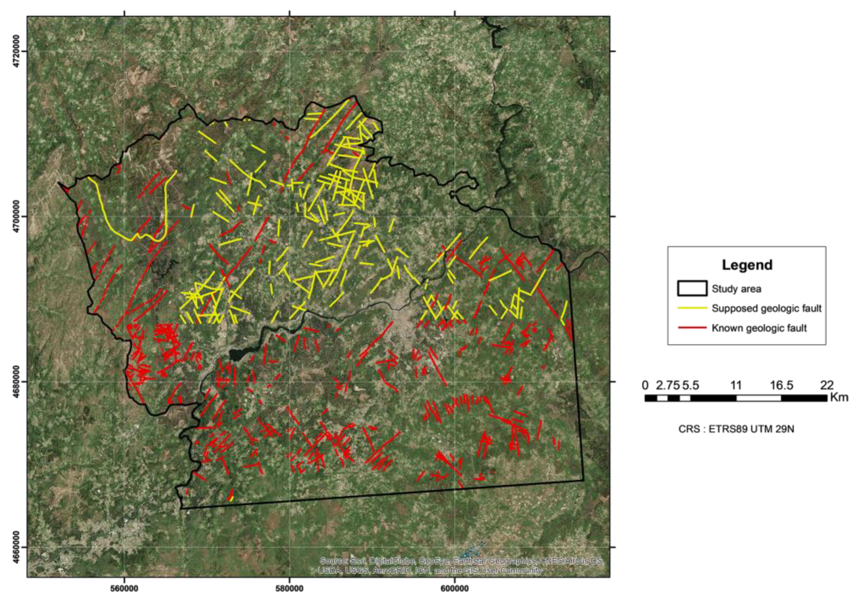
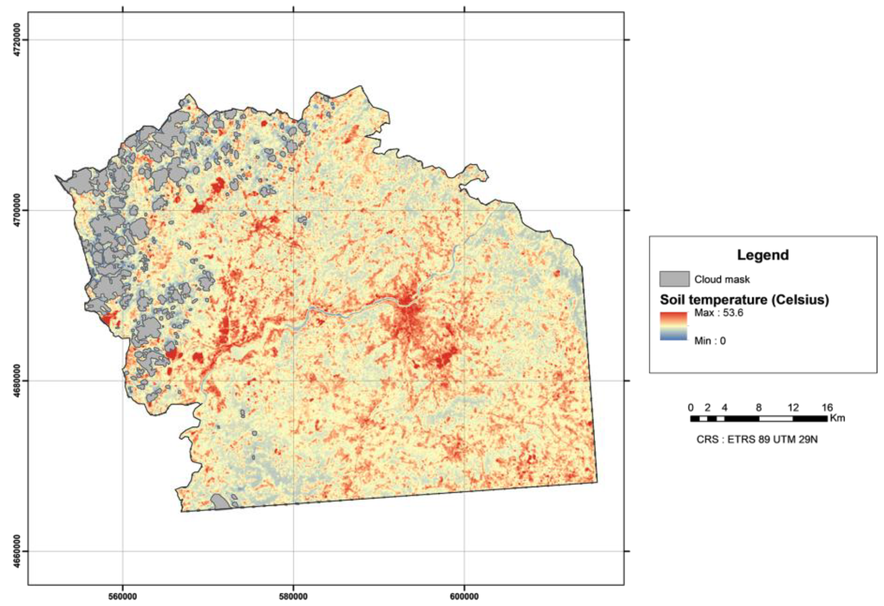
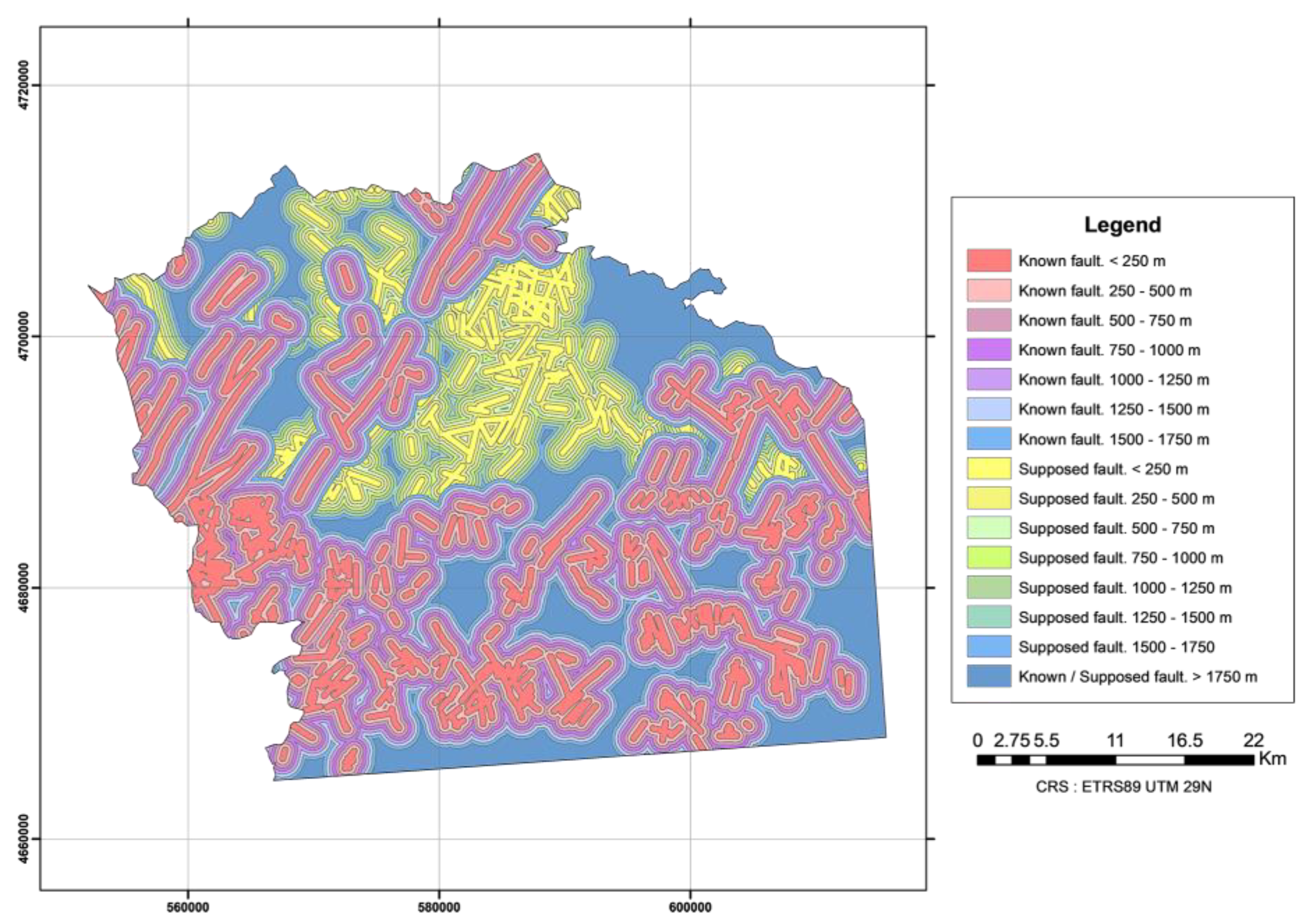
As for the geological faults map and the LST map, it is difficult to associate them with the geothermal potential map directly. In the case of the geological faults map (Figure 8), both known and unknown faults are distributed all over the study area in areas occupied by different types of geothermal potential classes. In the case of the LST map (Figure 6) this is due to the fact that, as it was said before, the areas with the highest temperatures in the map correspond with areas of infrastructures, whereas in other areas the temperature variation is not enough to establish comparisons. The relationship between temperature in the subsoil and the surface using remote sensing techniques has been a goal of many works like [14,60] making it a reliable technique to apply in a geothermal study.
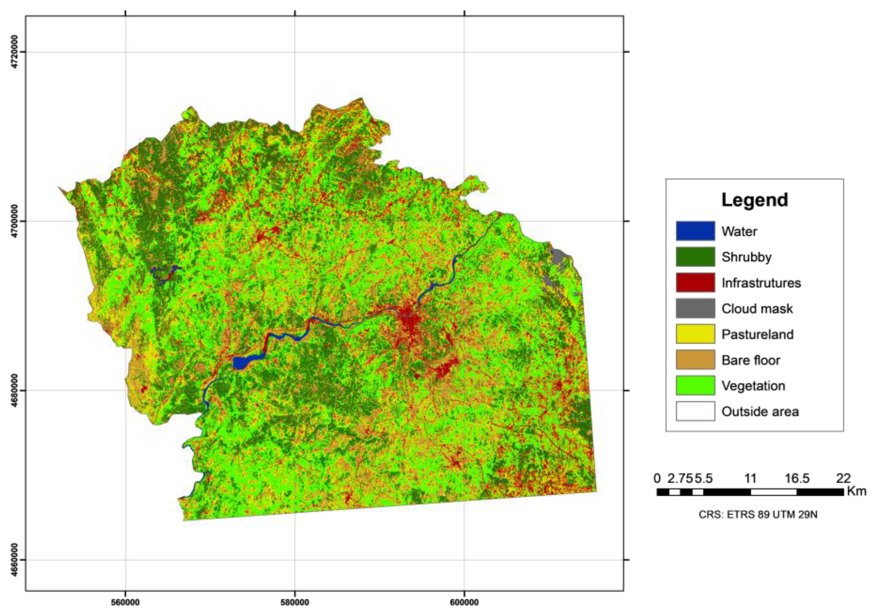
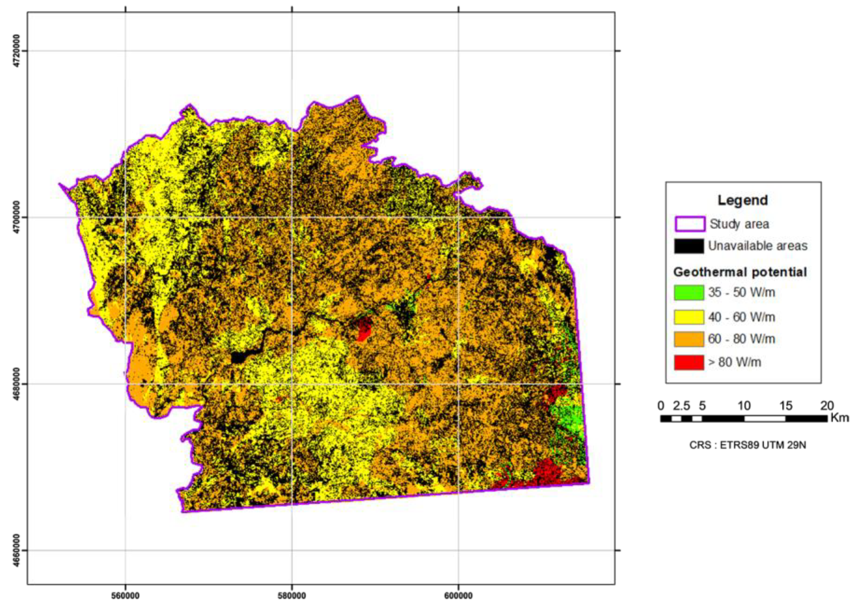
To refine the areas related to geothermal reservoirs, the land cover map was used to take into account those areas that cannot be exploited because they are occupied by infrastructures (roads, buildings, etc.) water and vegetation zones, and areas without reliable data, as the zones affected by the cloud cover during the image acquisition. As can be seen in Figure 12 and in Table 5, the number of potential zones has been reduced to almost half for the classes 35–50 W·m−1 and 40–60 W·m−1.
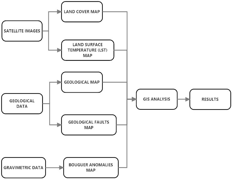
To assess the influence of the various elements of the presented workflow in the detecting ability of areas of geothermal potential, a sensitivity study was carried out. It aimed to highlight the importance the various features (see Figure 1) in detecting locations with the RF classifier.
It was considered a total of six combinations with three elements, namely: geological map, faults, and gravimetric anomalies. The land cover and LST map are included always in the assessment. A RF classification with a depth = 8 and number of trees = 100 trees was applied with a k-fold cross-validation with k = 10. In Table 6, the overall accuracy, the Kappa index, and the area under the ROC curve (AUC) for the six combinations, as well as the reference are reported.
As it is shown in the previous table, there is a common behavior for the three variables considered. The faults’ influence zone is the class with the lowest influence in the final results, lowering the Kappa index about 5.4% when it is absent. However, when the geological map or the gravimetric anomalies do not participate in the classification the Kappa index worsens between 14.2% and 16.0% respectively. In the last three rows of Table 6 the effect is shown when only three variables are considered: The land cover and LST map plus the highlighted variable. First of all, the results when only the faults are taken into account are very significant, yielding results similar to a random classification (Kappa = 0, and AUC = 0.5). Secondly, the geological map plays the most significant role, with a decrease of the Kappa index of only 16.6%, whereas the AUC remains approximately 90%. Finally, the inclusion of the gravimetric anomalies is not sufficient for an adequate classification, as stated by the low Kappa index (56%).
In order to assess the ability of the RF algorithm to forecast the geothermal potential, the proposed methodology is tested, training the RF classifier with a non-random subset of the training polygons. Next, the overall accuracy of the rest of the ground truth information, which has stayed completely unknown to the RF during training, is quantified. So, the RF is trained using only the training polygons located in the southeast quadrant of the study area, where the four classes of geothermal potential are present. A total of 171 polygons are considered, namely 30% of the original set. The RF configuration remains the same: depth = 8, number of trees = 100, and a k-fold validation with k = 10. The RF classification for the cross-validation achieved a Kappa index of 86.4%, an overall accuracy of 92.7%, and an AUC equal to 98.6%. These values are pretty similar to those obtained for the complete study area (see previous section). The subset RF classification is applied to the southeast quadrant of 529.8 km2 (23.8% of the total area of the study region). Next, the trained classifier is applied to areas progressively larger up to the complete study region (2227.31 km2). The overall accuracy and Kappa index for the different areas is evaluated in relation to the original RF classification (Figure 11a) as shown in Table 7.
As shown in Table 7, the results of the subset RF classification diverges from the reference classification (Figure 11a) proportionally to the distance from the training area. It is significant that the Kappa index decrease abruptly when the tested region is about 2.8 times the trained area and then the values decrease with a soft trend. For predictions up to 2.1 times the original training area, the proposed methodology is able to achieve an adequate classification with a Kappa > 75% [61,62].
As future lines of improvement, the enhancement of the initial dataset, as for example the generation of gravimetric anomalies by field observations, for a fine detection of geothermal potential zones, is recommended. Another improvement would be a geological survey of the study area, which would imply an enrichment of the geological classes as well as the reclassified informational classes. However, the potential improvement of the final precision will imply a significant increase in the cost of the approach; by these reasons, the present research, based on open/free data sources, provides an optimal baseline according to the authors.
The addition of data related to aquifer zones would allow obtaining the areas suitable for the exploitation of geothermal energy through vertical circuits, which take advantage of geothermal energy by taking and reinjecting water from aquifers. The thermal data would be improved by satellite night thermal images that would allow the ability to compare with the day images, and to derive thermal inertia maps.
Finally, it would be of interest to carry out geothermal drill tests in the areas identified with great geothermal potential, in addition to several samples in other areas spread over the study area, to validate the technique and the results obtained.

5. Conclusions

The use of geomatic techniques, such as remote sensing and geographical information systems allowed obtaining areas of geothermal potential in a simple way. The Sentinel-2A images allowed the creation of a land cover map in a detailed spatial resolution (between 10 and 20 m) and with zero cost. However, the use of these images together with the use of a spectral signature library did not allow the creation of a geological map as expected in the early stages of the work (probably due to the variation of conditions in the data acquisition and the library ones). Another factor related to this limitation is the scarce number of bands in the mid-infrared region, where it is easier to differentiate rocks [63]. The other image set employed (from ASTER), allowed the ability to obtain maps of soil temperatures at a fairly detailed spatial resolution (90 m) for a thermal sensor, and without any acquisition cost. The gravimetric anomalies, such as the Bouguer anomalies employed in the present work, are suitable for the search of geothermal potential areas due to their relationship with aquifer zones. Finally, the use of random forest eased the decision making in projects with a large amount of different and complex data, and where categorical and continuous data are mixed.
To incorporate geothermal resources into the energy network, it is necessary to optimize energy distribution and service organization. The availability of spatial information on the geothermal capacities of each zone allows the optimization of the energy network in terms of efficiency. Since the drilling costs are important, the identification of the reservoirs with higher potential will allow the reduction of these costs, such as the drilling length or the number of drill tests. The proposed workflow allows an easy generalization to different scenarios and regions and can be enriched with additional information layers.

Author Contributions

Conceptualization, P.R.-G. and D.L.G.; methodology, D.L.G. and P.R.-G.; validation, D.L.G.; formal analysis, D.L.G. and P.R.-G.; investigation, D.L.G. and P.R.-G.; writing—original draft preparation, P.R.-G. and D.L.G.; writing—review and editing, P.R.-G.; supervision, P.R.-G.

Funding

This research received no external funding.

Conflicts of Interest

The authors declare no conflict of interest.

References

  1. International Energy Agency (IEA). World Energy Balances 2018. Available online: https://webstore.iea.org/world-energy-balances-2018 (accessed on 18 August 2019).
  2. Mediavilla, M.; de Castro, C.; Capellán, I.; Miguel, L.J.; Arto, I.; Frechoso, F. The transition towards renewable energies: Physical limits and temporal conditions. Energy Policy 2013, 52, 297–311. [Google Scholar] [CrossRef]
  3. Council of the European Commission. Directive 2009/28/EC of the European Parliament and of the council of 23 April 2009 on the promotion of the use of energy from renewable sources and amending and subsequently repealing Directives 2001/77/EC and 2003/30/EC. Off. J. Eur. Union 2009, 140, 16–62. [Google Scholar]
  4. Stylianou, I.I.; Florides, G.; Tassou, S.; Tsiolakis, E.; Christodoulides, P. Methodology for estimating the ground heat absorption rate of Ground Heat Exchangers. Energy 2017, 127, 258–270. [Google Scholar] [CrossRef]
  5. Alhamid, M.I.; Daud, Y.; Surachman, A.; Sugiyono, A.; Aditya, H.B.; Mahlia, T.M.I. Potential of geothermal energy for electricity generation in Indonesia: A review. Renew. Sustain. Energy Rev. 2016, 53, 733–740. [Google Scholar] [CrossRef]
  6. Armannsson, H.; Fridriksson, T.; Kristjánsson, B.R. CO2 emissions from geothermal power plants and natural geothermal activity in Iceland. Geothermics 2005, 34, 286–296. [Google Scholar] [CrossRef]
  7. Kristensen, L.; Hjuler, M.L.; Frykman, P.; Olivarius, M.; Weibel, R.; Nielsen, L.H.; Mathiesen, A. Pre-drilling assessments of average porosity and permeability in the geothermal reservoirs of the Danish area. Geotherm. Energy 2016, 4, 6. [Google Scholar] [CrossRef]
  8. Howari, F. Prospecting for geothermal energy through satellite based thermal data: Review and the way forward. Glob. J. Environ. Sci. Manag. 2015, 1, 265–274. [Google Scholar] [CrossRef]
  9. Macharia, M.W.; Gachari, M.K.; Kuria, D.N.; Mariita, N.O. Low cost geothermal energy indicators and exploration methods in Kenya. J. Geogr. Reg. Plan. 2017, 10, 254–265. [Google Scholar] [CrossRef]
  10. Calvin, W.M.; Littlefield, E.F.; Kratt, C. Remote sensing of geothermal-related minerals for resource exploration in Nevada. Geothermics 2015, 53, 517–526. [Google Scholar] [CrossRef] [Green Version]
  11. Coolbaugh, M.F.; Kratt, C.; Fallacaro, A.; Calvin, W.M.; Taranik, J.V. Detection of geothermal anomalies using advanced spaceborne thermal emission and reflection radiometer (ASTER) thermal infrared images at Bradys Hot Springs, Nevada, USA. Remote Sens. Environ. 2007, 106, 350–359. [Google Scholar] [CrossRef]
  12. Van der Meer, F.D.; Van der Werff, H.M.A.; Van Ruitenbeek, F.J.A. Potential of ESA’s Sentinel-2 for geological applications. Remote Sens. Environ. 2014, 148, 124–133. [Google Scholar] [CrossRef]
  13. Qin, Q.; Zhang, N.; Nan, P.; Chai, L. Geothermal area detection using Landsat ETM+ thermal infrared data and its mechanistic analysis—A case study in Tengchong, China. Int. J. Appl. Earth Obs. Geoinf. 2011, 13, 552–559. [Google Scholar] [CrossRef]
  14. Li, J.; Zhang, Y. GIS-supported certainty factor (CF) models for assessment of geothermal potential: A case study of Tengchong County, southwest China. Energy 2017, 140, 552–565. [Google Scholar] [CrossRef]
  15. Yu, Z.; Haghighat, F.; Fung, B.C.; Yoshino, H. A decision tree method for building energy demand modeling. Energy Build. 2010, 42, 1637–1646. [Google Scholar] [CrossRef] [Green Version]
  16. Ahmad, M.W.; Reynolds, J.; Rezgui, Y. Predictive modelling for solar thermal energy systems: A comparison of support vector regression, random forest, extra trees and regression trees. J. Clean. Prod. 2018, 203, 810–821. [Google Scholar] [CrossRef]
  17. Congedo, L. Semi-Automatic Classification Plugin Documentation. Available online: http://semiautomaticclassificationmanual-v5.readthedocs.io/en/latest/remote_sensing.html#dos1-correction (accessed on 18 August 2019).
  18. GDAL/OGR contributors. GDAL/OGR Geospatial Data Abstraction software Library. Open Source Geospatial Foundation. Available online: http://gdal.org (accessed on 18 August 2019).
  19. Chavez, P.S. Image-based atmospheric corrections-Revisited and improved. Photogramm. Eng. Remote Sens. 1996, 62, 1025–1035. [Google Scholar]
  20. Sobrino, J.A.; Jimenez-Muñoz, J.C.; Paolini, L. Land surface temperature retrieval from LANDSAT TM 5. Remote Sens. Environ. 2004, 90, 434–440. [Google Scholar] [CrossRef]
  21. Moran, M.S.; Jackson, R.D.; Slater, P.N.; Teillet, P.M. Evaluation of simplified procedures for retrieval of land surface reflectance factors from satellite sensor output. Remote Sens. Environ. 1992, 41, 169–184. [Google Scholar] [CrossRef]
  22. Bharathkumar, L.; Mohammed-Aslam, M.A. Crop pattern mapping of Tumkur taluk using NDVI technique: A remote sensing and GIS approach. Aquat. Procedia 2015, 4, 1397–1404. [Google Scholar] [CrossRef]
  23. Jensen, J.R. Introductory Digital Image Processing: A Remote Sensing Perspective; Prentice Hall Press: Upper Saddle River, NJ, USA, 2015. [Google Scholar]
  24. Chuvieco Salinero, E. Teledetección Ambiental: La Observación de la TIERRA Desde el Espacio; Ariel: Barcelona, Spain, 2006. [Google Scholar]
  25. Sauro, J.; Lewis, J.R. Estimating completion rates from small samples using binomial confidence intervals: Comparisons and recommendations. In Proceedings of the human factors and ergonomics society annual meeting, Orlando, FL, USA, 26–30 September 2005; Sage: Los Angeles, CA, USA, 2005; pp. 2100–2103. [Google Scholar]
  26. Lewis, J.R.; Sauro, J. When 100% really isn’t 100%: Improving the accuracy of small-sample estimates of completion rates. J. Usability Stud. 2006, 1, 136–150. [Google Scholar]
  27. Measuring, U. Confidence Interval Calculator for a Completion Rate. Available online: https://measuringu.com/wald/ (accessed on 18 August 2019).
  28. Fridleifsson, I.B.; Bertani, R.; Huenges, E.; Lund, J.W.; Ragnarsson, A.; Rybach, L. The possible role and contribution of geothermal energy to the mitigation of climate change. In Proceedings of the IPCC Scoping Meeting on Renewable Energy Sources, Lübeck, Germany, 20–25 January 2008; pp. 59–80. [Google Scholar]
  29. Sameen, M.I.; Al Kubaisy, M.A. Automatic surface temperature mapping in Arcgis using landsat-8 TIRS and ENVI tools, case study: Al Habbaniyah Lake. J. Environ. Earth Sci. 2014, 4, 12–17. [Google Scholar]
  30. Zhibin, R.; Haifeng, Z.; Xingyuan, H.; Dan, Z.; Xingyang, Y. Estimation of the relationship between urban vegetation configuration and land surface temperature with remote sensing. J. Indian Soc. Remote Sens. 2015, 43, 89–100. [Google Scholar] [CrossRef]
  31. Hook, S.J.; Gabell, A.R.; Green, A.A.; Kealy, P.S. A comparison of techniques for extracting emissivity information from thermal infrared data for geologic studies. Remote Sens. Environ. 1992, 42, 123–135. [Google Scholar] [CrossRef]
  32. Gillespie, A.R. A new approach for temperature and emissivity separation. Int. J. Remote Sens. 2000, 21, 2127–2132. [Google Scholar] [CrossRef]
  33. Tarbuck, E.J.; Lutgens, F.K. Ciencias de la Tierra; Pearson Prentice Hall: Madrid, Spain, 2005. [Google Scholar]
  34. Spanish Geological Survey. Vocabulary of Rocks, Sediments and Surface Formations. Available online: http://info.igme.es/SidPDF/167000/386/167386_0000001.pdf (accessed on 18 August 2019).
  35. Hackney, R.I.; Featherstone, W.E. Geodetic versus geophysical perspectives of the ‘gravity anomaly’. Geophys. J. Int. 2003, 154, 35–43. [Google Scholar] [CrossRef]
  36. Rochdane, S.; El Mandour, A.; Jaffal, M.; Himi, M.; Casas, A.; Amrhar, M.; Karroum, M. Geometry of the eastern Haouz and Tassaout aquifers, Western Morocco: Geophysical and hydrogeological approach. Hydrol. Sci. J. 2015, 6, 133–144. [Google Scholar] [CrossRef]
  37. Hofmann-Wellenhof, B.; Moritz, H. Physical Geodesy; Springer Science & Business: Media, Austria, 2006. [Google Scholar]
  38. Pasteka, R.; Mikuska, J.; Meurers, B. Understanding the Bouguer Anomaly: A Gravimetry Puzzle; Elsevier: Amsterdam, The Netherlands, 2017. [Google Scholar]
  39. O’Neil, G.L.; Goodall, J.L.; Watson, L.T. Evaluating the potential for site-specific modification of LiDAR DEM derivatives to improve environmental planning-scale wetland identification using Random Forest classification. J. Hydrol. 2018, 559, 192–208. [Google Scholar] [CrossRef]
  40. Rodriguez-Galiano, V.F.; Ghimire, B.; Rogan, J.; Chica-Olmo, M.; Rigol-Sanchez, J.P. An assessment of the effectiveness of a random forest classifier for land-cover classification. Isprs J. Photogramm. Remote Sens. 2012, 67, 93–104. [Google Scholar] [CrossRef]
  41. Drusch, M.; Del Bello, U.; Carlier, S.; Colin, O.; Fernandez, V.; Gascon, F.; Meygret, A. Sentinel-2: ESA’s optical high-resolution mission for GMES operational services. Remote Sens. Environ. 2012, 120, 25–36. [Google Scholar] [CrossRef]
  42. Abrams, M. The Advanced Spaceborne Thermal Emission and Reflection Radiometer (ASTER): Data products for the high spatial resolution imager on NASA’s Terra platform. Int. J. Remote Sens. 2000, 21, 847–859. [Google Scholar] [CrossRef]
  43. Spanish Geological Survey. MAGNA 50-Geological Map of Spain, Scale 1:50.000. Available online: http://info.igme.es/cartografiadigital/geologica/Magna50.aspx?language=en (accessed on 18 August 2019).
  44. Llopis, G.; Rodrigo, V. Guía de la Energía Geotérmica; Dirección general de la industria energía, y minas, consejería de economía y consumo: Madird, Spain, 2008. [Google Scholar]
  45. Bellani, S.; Brogi, A.; Lazzarotto, A.; Liotta, D.; Ranalli, G. Heat flow, deep temperatures and extensional structures in the Larderello Geothermal Field (Italy): Constraints on geothermal fluid flow. J. Volcanol. Geotherm. Res. 2004, 132, 15–29. [Google Scholar] [CrossRef]
  46. Taillefer, A.; Soliva, R.; Guillou-Frottier, L.; Le Goff, E.; Martin, G.; Seranne, M. Fault-related controls on upward hydrothermal flow: An integrated geological study of the Têt fault system, Eastern Pyrénées (France). Geofluids 2017, 2017, 8190109. [Google Scholar] [CrossRef]
  47. Bureau Gravimetrique International (BGI). 10.18168/BGI. Available online: http://bgi.omp.obs-mip.fr/data-products/Gravity-Databases/Land-Gravity-data (accessed on 16 October 2019).
  48. Urpelainen, J.; Van de Graaf, T. The International Renewable Energy Agency: A success story in institutional innovation? Int. Environ. Agreem. Pol. Law Econ. 2015, 15, 159–177. [Google Scholar] [CrossRef]
  49. International Renewable Energy Agency (IRENA). Available online: https://irena.masdar.ac.ae/geoserver/ows?service=wms&version=1.3.0&request=GetCapabilities (accessed on 18 August 2019).
  50. Spanish Institute for the Diversification and Saving of Energy (IDEA). Available online: http://www.idae.es/ (accessed on 18 August 2019).
  51. Colmenar-Santos, A.; Folch-Calvo, M.; Rosales-Asensio, E.; Borge-Diez, D. The geothermal potential in Spain. Renew. Sustain. Energy Rev. 2016, 56, 865–886. [Google Scholar] [CrossRef]
  52. European Space Agency (ESA). Copernicus Open Access Hub. Available online: https://scihub.copernicus.eu/ (accessed on 18 August 2019).
  53. National Aeronautics and Space Administration (NASA). Earth Observation Data. Available online: https://earthdata.nasa.gov/ (accessed on 18 August 2019).
  54. Bakar, Z.A.; Mohemad, R.; Ahmad, A.; Deris, M.M. A comparative study for outlier detection techniques in data mining. In Proceedings of the 2006 IEEE Conference on Cybernetics and Intelligent Systems, Bangkok, Thailand, 7–9 June 2006. [Google Scholar] [CrossRef]
  55. Rymer, H.; Brown, G.C. Gravity fields and the interpretation of volcanic structures: Geological discrimination and temporal evolution. J. Volcanol. Geotherm. Res. 1986, 27, 229–254. [Google Scholar] [CrossRef]
  56. Ebrahimi, D.; Nouraliee, J.; Dashti, A. Assessing the geothermal potential of the Shahin Dezh Region, based on the geological, geochemical and geophysical evidence. J. Afr. Earth Sci. 2019, 152, 84–89. [Google Scholar] [CrossRef]
  57. Romaguera, M.; Vaughan, R.G.; Etterma, J.; Izquierdo-Verdiguier, E.; Hecker, C.A. Detecting geotermal anomalies and evaluating LST geotermal component by combining termal remote sensing time series and land Surface model data. Remote Sens. Environ. 2018, 204, 534–552. [Google Scholar] [CrossRef]
  58. Stone, M. Cross-validatory choice and assessment of statistical predictions. J. R. Stat. Soc. 1974, 3, 111–147. [Google Scholar] [CrossRef]
  59. Bradley, A.P. The use of the area under the ROC curve in the evaluation of machine learning algorithms. Pattern Recognit. 1997, 30, 1145–1159. [Google Scholar] [CrossRef] [Green Version]
  60. Hempstalk, K.; Frank, E.; Witten, I.H. One-class classification by combining density and class probability estimation. In Proceedings of the Joint European Conference on Machine Learning and Knowledge Discovery in Databases, Antwerp, Belgium, 15–19 September 2008. [Google Scholar] [CrossRef]
  61. Foody, G.M. Harshness in image classification accuracy assessment. Int. J. Remote Sens. 2008, 29, 3137–3158. [Google Scholar] [CrossRef] [Green Version]
  62. Rodríguez-Gonzálvez, P.; Rodríguez-Martín, M. Weld Bead Detection Based on 3D Geometric Features and Machine Learning Approaches. IEEE Access 2019, 7, 14714–14727. [Google Scholar] [CrossRef]
  63. Del Pozo, S.; Lindenbergh, R.; Rodríguez-Gonzálvez, P.; Blom, J.K.; González-Aguilera, D. Discrimination between sedimentary rocks from close-range visible and very-near-infrared images. PLoS ONE 2015, 10, e0132471. [Google Scholar] [CrossRef] [PubMed]
Figure 1. Research workflow.
Remotesensing 11 02403 g001
Figure 2. Map of geological faults.
Remotesensing 11 02403 g002
Figure 3. Distribution the training areas on the Web Map Service of the International Renewable Energy Agency (IRENA) [49].
Remotesensing 11 02403 g003
Figure 4. Location of study case. The study area is highlighted in red stripes.
Remotesensing 11 02403 g004
Figure 5. Land cover map.
Remotesensing 11 02403 g005
Figure 6. Land surface temperature map.
Remotesensing 11 02403 g006
Figure 7. Geological map with the six reclassified informational classes.
Remotesensing 11 02403 g007
Figure 8. Geological fault and influence zones map.
Remotesensing 11 02403 g008
Figure 9. Bouguer gravimetric anomaly map.
Remotesensing 11 02403 g009
Figure 10. Geothermal potential map.
Remotesensing 11 02403 g010
Figure 11. Geothermal potential map (a) and ground truth (b).
Remotesensing 11 02403 g011
Figure 12. Geothermal potential areas refined on the basis of the land cover map.
Remotesensing 11 02403 g012
Table 1. Description of the reclassified geological classes from the Spanish national geological map.
ClassDescription
Intrusive plutonic rockSolidified igneous rock inside the Earth’s crust, from a silicated magma.
Intrusive igneous rockRock originated by the solidification of a silicated magma inside the Earth’s crust at a shallow depth (not exceeding 3 km).
Extrusive or volcanic igneous rockIgneous rock produced by activity volcanic, usually of very fine or vitreous grain.
Metamorphic rockRock derived from a pre-existing rock, through mineralogical, chemical or structural changes, in response to physicochemical variations, mainly of pressure and temperature (there are excluded the rocks derived from processes of weathering or soil formation).
Detrital sedimentary rockRock formed from a solid element that has been weathered by air or water, and may undergo changes when exposed to temperature or pressure.
Unconsolidated sedimentSolid material that was formed by secondary sedimentation of previously weathered rocks, and/or by chemical and biochemical precipitation.
Table 2. Confusion matrix of maximum likelihood classification for the Sentinel-2 image #3.
True ValueUser acc. (%)Confidence Interval (%)
ClassesPast.WaterShrubbyBare F.Infra.Veg.Total
Predicted valuePast.69000047394.586.3–98.3
Water065000065100.095.2–100
Shrubby03670047490.581.5–95.6
Bare F.00354506287.176.3–93.6
Infra010166508279.369.2–86.7
Veg.11000626497.088.7–99.8
Total707070707070420
Producer acc. (%)98.692.995.777.192.988.6
Confidence interval (%)91.6–99.984.0–97.387.7–99.065.9–85.584.0–97.378.8–94.3
Table 3. Number of training areas for each class for the final classification.
Geothermal PotentialN° Training Polygons
35–50 W·m−132
40–60 W·m−1274
60–80 W·m−1209
>80 W·m−154
Table 4. Surface occupied by each geothermal potential class.
Geothermal PotentialPixel CountArea (km2)
35–50 W·m−1370630.02
40–60 W·m−195,672774.94
60–80 W·m−1171,5341389.42
>80 W·m−1410333.23
Table 5. Surface occupied by each geothermal potential class refined on the basis of the land cover map.
Geothermal PotentialPixel CountArea (km2)
35–50 W·m−1207716.82
40–60 W·m−161,198495.70
60–80 W·m−198,302796.24
>80 W·m−1217617.62
Table 6. Sensitivity analysis. Results of a k-fold cross-validation (k = 10) of a random forest classification (depth = 8 and number of trees = 100).
Variable TestedClassification Results
Geological MapFaultsGravimetric AnomaliesOverall AccuracyKappa IndexAUC
REFERENCEYesYesYes94.0%88.4%98.7%
YesYesNo86.8%74.3%92.6%
YesNoYes91.6%83.6%97.6%
NoYesYes87.7%75.8%95.9%
YesNoNo86.4%73.8%90.3%
NoYesNo62.0%18.6%66.8%
NoNoYes78.6%56.0%90.5%
Table 7. Results of random forest (RF) classification trained with a non-random partial subset in relation to the RF trained with the complete study area.
Area (km2)Area IncrementOverall AccuracyKappa Index
529.80-93.1%86.6%
817.0754.2%88.7%78.7%
1134.98114.2%86.7%73.7%
1480.97179.5%83.3%57.8%
1800.40239.8%79.8%57.8%
2087.26294.0%78.1%55.1%
2227.31320.4%77.3%54.0%

