Rapid and Accurate Monitoring of Intertidal Oyster Reef Habitat Using Unoccupied Aircraft Systems and Structure from Motion


Abstract

1. Introduction
2. Methods
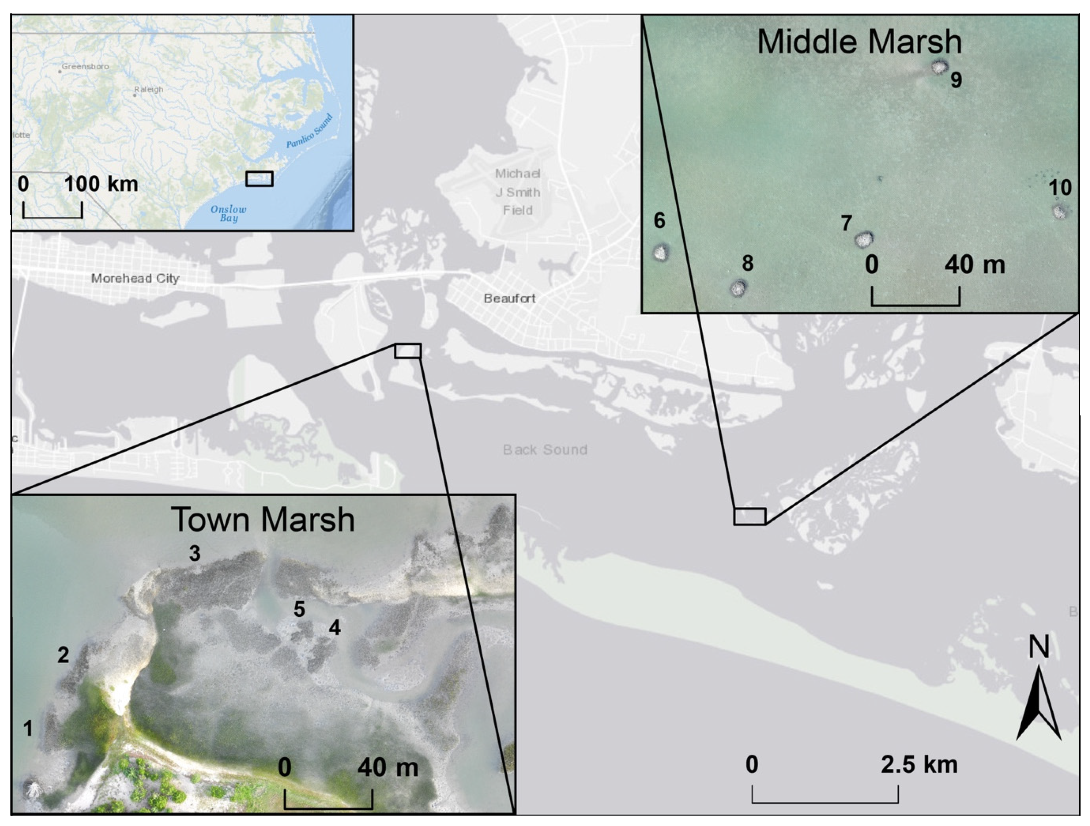
2.1. Study Area
2.2. Traditional Field Surveys
2.3. Unoccupied Aircraft Systems
2.4. Remote Sensing Evaluation Methods
2.5. Statistical Analysis
3. Results
3.1. Initial Processing and GCP Correction
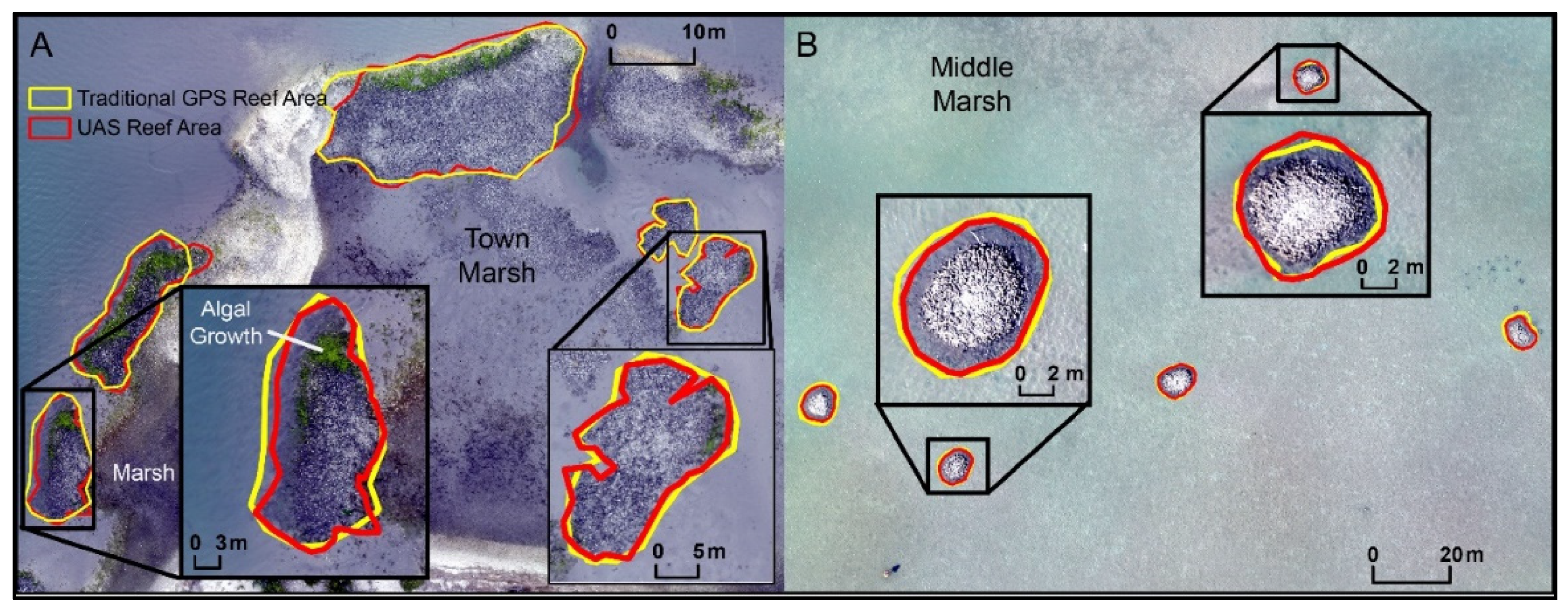
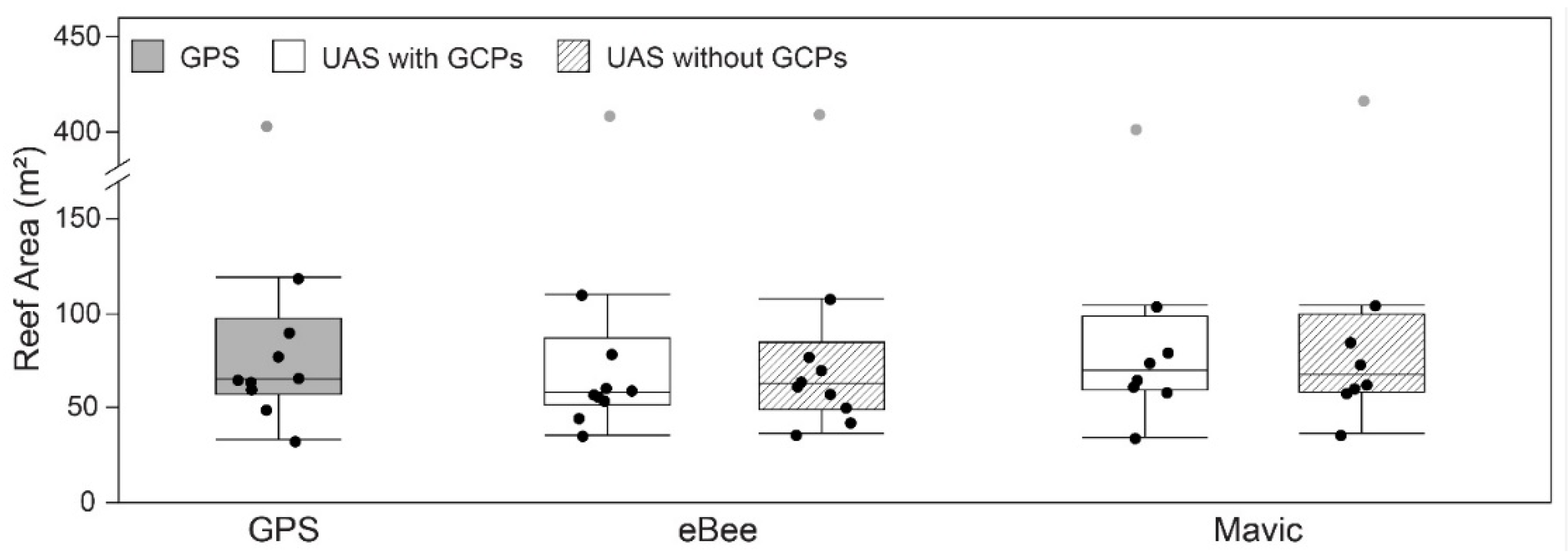
3.2. Reef Area
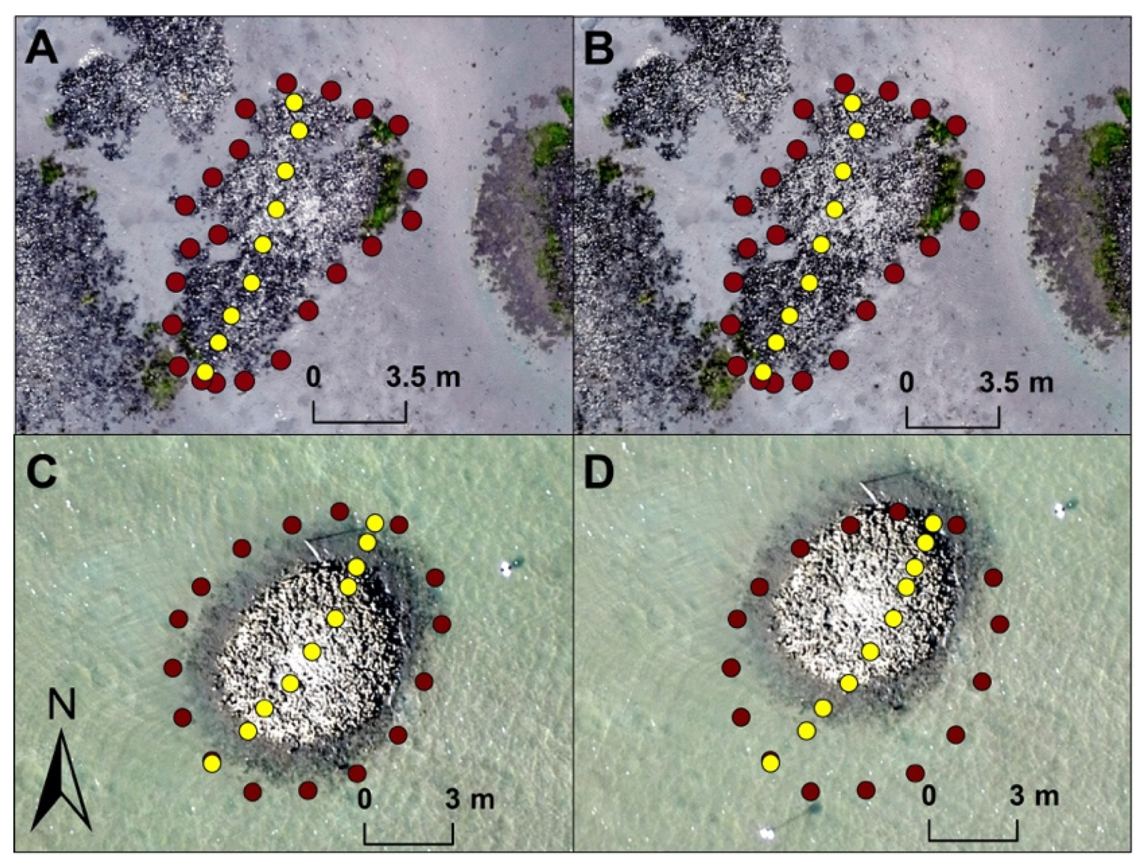
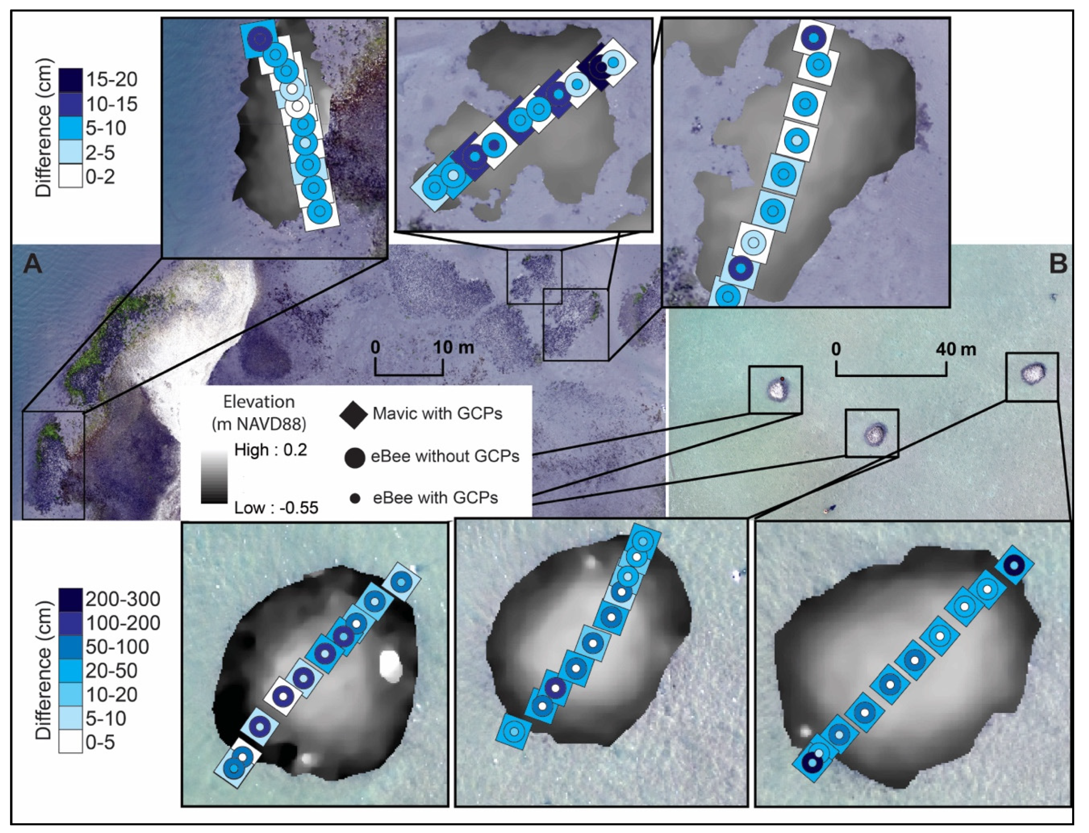
3.3. Reef Morphology
4. Discussion
4.1. Reef Area
4.2. Reef Morphology
4.3. Broader Implications
5. Conclusions
Supplementary Materials
Author Contributions
Funding
Acknowledgments
Conflicts of Interest
References
- Coen, D.L.; Humphries, A. Oyster-generated marine habitats: Their services, enhancement, restoration, and monitoring. In Routledge Handbook of Ecological and Environmental Restoration; Murphy, S., Allison, S., Eds.; Taylor & Francis Group/Routledge: Cambridge, UK, 2017; pp. 275–295. [Google Scholar]
- Grabowski, J.H.; Brumbaugh, R.D.; Conrad, R.F.; Keeler, A.G.; Opaluch, J.J.; Peterson, C.H.; Piehler, M.F.; Powers, S.P.; Smyth, A.R. Economic valuation of ecosystem services provided by oyster reefs. BioScience 2012, 62, 900–909. [Google Scholar] [CrossRef]
- Kellogg, M.L.; Smyth, A.R.; Luckenbach, M.W.; Carmichael, R.H.; Brown, B.L.; Cornwell, J.C.; Piehler, M.F.; Owens, M.S.; Dalrymple, D.J.; Higgins, C.B. Use of oysters to mitigate eutrophication in coastal waters. Estuar. Coast. Shelf Sci. 2014, 151, 156–168. [Google Scholar] [CrossRef]
- McLeod, I.M.; zu Ermgassen, P.S.; Gillies, C.L.; Hancock, B.; Humphries, A. Can Bivalve Habitat Restoration Improve Degraded Estuaries? In Coasts and Estuaries; Elsevier: Amsterdam, The Netherlands, 2019; pp. 427–442. [Google Scholar]
- Smaal, A.C.; Ferreira, J.G.; Grant, J.; Petersen, J.K.; Strand, Ø. (Eds.) Goods and Services of Marine Bivalves; Springer: Berlin/Heidelberg, Germany, 2018. [Google Scholar]
- Ysebaert, T.; Walles, B.; Haner, J.; Hancock, B. Habitat modification and coastal protection by ecosystem-engineering reef-building bivalves. In Goods and Services of Marine Bivalves; Springer: Berlin/Heidelberg, Germany, 2019; pp. 253–273. [Google Scholar]
- Kirby, M.X. Fishing down the coast: historical expansion and collapse of oyster fisheries along continental margins. Proc. Natl. Acad. Sci. USA 2004, 101, 13096–13099. [Google Scholar] [CrossRef] [PubMed]
- zu Ermgassen, P.S.; Spalding, M.D.; Grizzle, R.E.; Brumbaugh, R.D. Quantifying the loss of a marine ecosystem service: Filtration by the eastern oyster in US estuaries. Estuaries Coasts 2013, 36, 36–43. [Google Scholar] [CrossRef]
- Airoldi, L.; Beck, M.W. Loss, status and trends for coastal marine habitats of Europe. In Oceanography and Marine Biology; CRC Press: Boca Raton, FL, USA, 2007; pp. 357–417. [Google Scholar]
- Lafferty, K.D.; Harvell, C.D.; Conrad, J.M.; Friedman, C.S.; Kent, M.L.; Kuris, A.M.; Powell, E.N.; Rondeau, D.; Saksida, S.M. Infectious diseases affect marine fisheries and aquaculture economics. Annu. Rev. Mar. Sci. 2015, 7, 471–496. [Google Scholar] [CrossRef] [PubMed]
- Wilberg, M.J.; Livings, M.E.; Barkman, J.S.; Morris, B.T.; Robinson, J.M. Overfishing, disease, habitat loss, and potential extirpation of oysters in upper Chesapeake Bay. Mar. Ecol. Prog. Ser. 2011, 436, 131–144. [Google Scholar] [CrossRef]
- zu Ermgassen, P.S.; Spalding, M.D.; Blake, B.; Coen, L.D.; Dumbauld, B.; Geiger, S.; Grabowski, J.H.; Grizzle, R.; Luckenbach, M.; McGraw, K.; et al. Historical ecology with real numbers: past and present extent and biomass of an imperiled estuarine habitat. Proc. R. Soc. B Biol. Sci. 2012, 279, 3393–3400. [Google Scholar] [CrossRef]
- Baggett, P.L.; Powers, S.P.; Brumbaugh, R.; Coen, L.D.; DeAngelis, B.; Greene, J.; Hancock, B.; Morlock, S. Oyster Habitat Restoration Monitoring and Assessment Handbook; The Nature Conservancy: Arlington, VA, USA, 2014; 96p. [Google Scholar]
- Brumbaugh, R.D.; Beck, M.W.; Coen, L.D.; Craig, L.; Hicks, P. A Practitioner’s Guide to the Design & Monitoring of Shellfish Restoration Projects: An Ecosystem Services Approach; The Nature Conservancy: Arlington, VA, USA, 2006. [Google Scholar]
- Coen, L.D.; Luckenbach, M.W. Developing success criteria and goals for evaluating oyster reef restoration: ecological function or resource exploitation? Ecol. Eng. 2000, 15, 323–343. [Google Scholar] [CrossRef]
- Oyster Metrics Workgroup (OMW). Restoration Goals, Quantitative Metrics and Assessment Protocols for Evaluating Success on Restored Oyster Reef Sanctuaries; Report of the Oyster Metrics Workgroup; Sustainable Fisheries Goal Implementation Team of the NOAA Chesapeake Bay Program: Annapolis, MD, USA, 2011; Available online: http://www.chesapeakebay.net/channel_files/ 17932/oyster_restoration_success_metrics_final.pdf (accessed on 15 August 2015).
- Coen, L.D.; Brumbaugh, R.D.; Bushek, D.; Grizzle, R.; Luckenbach, M.W.; Posey, M.H.; Powers, S.P.; Tolley, S.G. Ecosystem services related to oyster restoration. Mar. Ecol. Prog. Ser. 2007, 341, 303–307. [Google Scholar] [CrossRef]
- Grabowski, J.H.; Peterson, C.H. Restoring oyster reefs to recover ecosystem services. Ecosyst. Eng. Plants Protists 2007, 4, 281–298. [Google Scholar]
- Baggett, L.P.; Powers, S.P.; Brumbaugh, R.D.; Coen, L.D.; DeAngelis, B.M.; Greene, J.K.; Hancock, B.T.; Morlock, S.M.; Allen, B.L.; Breitburg, D.L.; et al. Guidelines for evaluating performance of oyster habitat restoration. Restor. Ecol. 2015, 23, 737–745. [Google Scholar] [CrossRef]
- Burrows, F.; Harding, J.M.; Mann, R.; Dame, R.; Coen, L. Chapter 4: Restoration monitoring of oyster reefs. In Science-Based Restoration Monitoring of Coastal Habitats; Thayer, G.W., McTigue, T.A., Salz, R.J., Merkey, D.H., Burrows, F.M., Gayaldo, P.F., Eds.; Volume Two: Tools for Monitoring Coastal Habitats; NOAA Coastal Ocean Program Decision Analysis Series No. 23; NOAA National Centers for Coastal Ocean Science: Silver Spring, MD, USA, 2005. [Google Scholar]
- Ridge, J.T.; Rodriguez, A.B.; Fodrie, F.J. Evidence of exceptional oyster-reef resilience to fluctuations in sea level. Ecol. Evol. 2017, 7, 11409–11420. [Google Scholar] [CrossRef] [PubMed]
- Ridge, J.T.; Rodriguez, A.B.; Fodrie, F.J.; Lindquist, N.L.; Brodeur, M.C.; Coleman, S.E.; Grabowski, J.H.; Theuerkauf, E.J. Maximizing oyster-reef growth supports green infrastructure with accelerating sea-level rise. Sci. Rep. 2015, 5, 14785. [Google Scholar] [CrossRef] [PubMed]
- Rodriguez, A.B.; Fodrie, F.J.; Ridge, J.T.; Lindquist, N.L.; Theuerkauf, E.J.; Coleman, S.E.; Grabowski, J.H.; Brodeur, M.C.; Gittman, R.K.; Keller, D.A.; et al. Oyster reefs can outpace sea-level rise. Nat. Clim. Chang. 2014, 4, 493–497. [Google Scholar] [CrossRef]
- Grizzle, R.E.; Adams, J.R.; Walters, L.J. Historical changes in intertidal oyster (Crassostrea virginica) reefs in a Florida lagoon potentially related to boating activities. J. Shellfish Res. 2002, 21, 749–756. [Google Scholar]
- Grizzle, R.; Ward, K.; Geselbracht, L.; Birch, A. Distribution and Condition of Intertidal Eastern Oyster (Crassostrea virginica) Reefs in Apalachicola Bay Florida Based on High-Resolution Satellite Imagery. J. Shellfish Res. 2018, 37, 1027–1039. [Google Scholar] [CrossRef]
- Twichell, D.C.; Andrews, B.D.; Edmiston, H.L.; Stevenson, W.R. Geophysical Mapping of Oyster Habitats in a Shallow Estuary, Apalachicola Bay, Florida: U.S. Geological Survey Open-File Report 2006-1381. 2007. Available online: http://pubs.usgs.gov/of/2006/1381/ (accessed on 1 May 2019).
- Walles, B.; Troost, K.; van den Ende, D.; Nieuwhof, S.; Smaal, A.C.; Ysebaert, T. From artificial structures to self-sustaining oyster reefs. J. Sea Res. 2016, 108, 1–9. [Google Scholar] [CrossRef]
- Power, A.; Corley, B.; Atkinson, D.; Walker, R.; Harris, D.; Manley, J.; Johnson, T. A caution against interpreting and quantifying oyster habitat loss from historical surveys. J. Shellfish Res. 2010, 29, 927–937. [Google Scholar] [CrossRef]
- Schill, S.R.; Porter, D.E.; Coen, L.D.; Bushek, D.; Vincent, J. Development of an automated mapping technique for monitoring and managing shellfish distributions. In NOAA/UNH Cooperative Institute for Coastal and Estuarine Environmental Technology (CICEET); University of New Hampshire: Durham, NH, USA, 2006; 91p. [Google Scholar]
- Nieuwhof, S.; Herman, P.M.; Dankers, N.; Troost, K.; Van Der Wal, D. Remote sensing of epibenthic shellfish using synthetic aperture radar satellite imagery. Remote Sens. 2015, 7, 3710–3734. [Google Scholar] [CrossRef]
- Garvis, S.K.; Sacks, P.E.; Walters, L.J. Formation, movement, and restoration of dead intertidal oyster reefs in Canaveral National Seashore and Mosquito Lagoon, Florida. J. Shellfish Res. 2015, 34, 251–258. [Google Scholar] [CrossRef]
- ASMFC. The Importance of Habitat Created by Molluscan Shellfish to Managed Species along the Atlantic Coast of the United States; Atlantic States Marine Fisheries Commission: Arlington County, VA, USA, 2007. [Google Scholar]
- Seavey, J.R.; Pine, W.E.; Frederick, P.; Sturmer, L.; Berrigan, M. Decadal changes in oyster reefs in the Big Bend of Florida’s Gulf Coast. Ecosphere 2011, 2, 1–14. [Google Scholar] [CrossRef]
- NOAA Coastal Services Center. Pilot Investigation of Remote Sensing for Intertidal Oyster Mapping in Coastal South Carolina: A Methods Comparison. 2003. Available online: https://coast.noaa.gov/data/digitalcoast/pdf/oyster-mapping.pdf (accessed on 16 September 2018).
- South Carolina Department of Natural Resources (SCDNR), Marine Resources Division. Final Report for South Carolina’s 2004-05 Intertidal Oyster Survey and Related Reef Restoration/Enhancement Program; NOAA Award No. NA04NMF4630309; South Carolina Department of Natural Resources (SCDNR), Marine Resources Division: Columbia, SC, USA, 2008. Available online: http://www.oyster-restoration.org/wp-content/uploads/2012/06/Final-Report-for-Oyster-Survey-and-Recovery-Phase-II-with-appendices.pdf (accessed on 16 September 2018).
- Guillen, G.; Mokrech, M. Mapping Shallow Reefs Using Low-Cost Scanning Sonar and Drone Photography Systems; EIH Final Report # 18-001; Environmental Institute of Houston: Houston, TX, USA, 2018. Available online: https://www.sciencebase.gov/catalog/item/5bf82b0fe4b045bfcae2eaae (accessed on 1 May 2019).
- Johnston, D.W. Unoccupied Aircraft Systems in Marine Science and Conservation. Ann. Rev. Mar. Sci. 2019, 11, 439–463. [Google Scholar] [CrossRef] [PubMed]
- Joyce, K.E.; Duce, S.; Leahy, S.M.; Leon, J.; Maier, S.W. Principles and practice of acquiring drone-based image data in marine environments. Mar. Freshw. Res. 2018, 70, 952–963. [Google Scholar] [CrossRef]
- Klemas, V.V. Coastal and environmental remote sensing from unmanned aerial vehicles: An overview. J. Coast. Res. 2015, 31, 1260–1267. [Google Scholar] [CrossRef]
- Mancini, F.; Dubbini, M.; Gattelli, M.; Stecchi, F.; Fabbri, S.; Gabbianelli, G. Using unmanned aerial vehicles (UAV) for high-resolution reconstruction of topography: The structure from motion approach on coastal environments. Remote Sens. 2013, 5, 6880–6898. [Google Scholar] [CrossRef]
- Seymour, A.C.; Ridge, J.T.; Rodriguez, A.B.; Newton, E.; Dale, J.; Johnston, D.W. Deploying fixed wing Unoccupied Aerial Systems (UAS) for coastal morphology assessment and management. J. Coast. Res. 2017, 34, 704–717. [Google Scholar] [CrossRef]
- R Core Team. R: A Language and Environment for Statistical Computing; R Foundation for Statistical Computing: Vienna, Austria, 2013. [Google Scholar]
- Le Bris, A.; Rosa, P.; Lerouxel, A.; Cognie, B.; Gernez, P.; Launeau, P.; Robin, M.; Barillé, L. Hyperspectral remote sensing of wild oyster reefs. Estuar. Coast. Shelf Sci. 2016, 172, 1–12. [Google Scholar] [CrossRef]
- O’Keife, K.; Arnold, W.; Reed, D. Tampa Bay oyster bar mapping and assessment. In Final Report to Tampa Bay Estuary Program; Technical Publication: Maharashtra, India, 2006. [Google Scholar]
- Casella, E.; Collin, A.; Harris, D.; Ferse, S.; Bejarano, S.; Parravicini, V.; Hench, J.L.; Rovere, A. Mapping coral reefs using consumer-grade drones and structure from motion photogrammetry techniques. Coral Reefs 2017, 36, 269–275. [Google Scholar] [CrossRef]
- Sturdivant, E.; Lentz, E.; Thieler, E.R.; Farris, A.; Weber, K.; Remsen, D.; Miner, S.; Henderson, R. UAS-SfM for coastal research: Geomorphic feature extraction and land cover classification from high-resolution elevation and optical imagery. Remote Sens. 2017, 9, 1020. [Google Scholar] [CrossRef]
- Yaney-Keller, A.; Tomillo, P.S.; Marshall, J.M.; Paladino, F.V. Using Unmanned Aerial Systems (UAS) to assay mangrove estuaries on the Pacific coast of Costa Rica. PLoS ONE 2019, 14, e0217310. [Google Scholar] [CrossRef]
- Burns, J.H.R.; Delparte, D.; Gates, R.D.; Takabayashi, M. Integrating structure-from-motion photogrammetry with geospatial software as a novel technique for quantifying 3D ecological characteristics of coral reefs. Peer J. 2015, 3, e1077. [Google Scholar] [CrossRef] [PubMed]


| Reef | GPS | eBee | Mavic | ||
|---|---|---|---|---|---|
| Area | Area | ΔGPS-eBee | Area | ΔGPS-Mavic | |
| Town Marsh (m2) | |||||
| 1 | 90.57 | 79.15 | 11.42 (12.61%) | 80.00 | 10.57 (11.67%) |
| 2 | 119.33 | 110.55 | 8.78 (7.36%) | 104.38 | 14.95 (12.53%) |
| 3 | 402.41 | 407.87 | 5.46 (1.36%) | 400.78 | 1.64 (0.41%) |
| 4 | 64.39 | 57.746 | 6.64 (10.32%) | 58.94 | 5.45 (8.46%) |
| 5 | 33.03 | 35.85 | 2.82 (8.54%) | 34.69 | 1.66 (5.03%) |
| Average ± S.D. | 7.02 ± 3.27 | 6.85 ± 5.82 | |||
| RMSE | 7.61 | 8.61 | |||
| Middle Marsh (m2) | |||||
| 6 | 77.92 | 61.19 | 16.73 (21.47%) | 74.54 | 3.38 (4.34%) |
| 7 | 66.47 | 59.85 | 6.62 (9.96%) | 65.42 | 1.05 (1.58%) |
| 8 | 65.51 | 56.65 | 8.86 (13.52%) | 61.88 | 3.63 (5.54%) |
| 9 | 60.46 | 54.47 | 5.99 (9.91%) | NA | NA |
| 10 | 49.64 | 45.23 | 4.41 (8.88%) | NA | NA |
| Average ± S.D. | 6.47 ± 1.85 | 2.69 ± 1.83 | |||
| RMSE | 9.57 | 2.93 | |||
| eBee | Mavic | ||||||
|---|---|---|---|---|---|---|---|
| Reef # | GPS | Corrected | Uncorrected | ΔGPS-Corrected | ΔGPS-Uncorrected | Corrected | ΔGPS-Corrected |
| Town Marsh (m) | |||||||
| 1 | –0.23 | –0.18 | –0.16 | 0.05 | 0.07 | –0.23 | 0.02 |
| 2 | –0.17 | –0.12 | –0.11 | 0.05 | 0.07 | –0.18 | 0.02 |
| 3 | –0.11 | –0.08 | –0.06 | 0.03 | 0.05 | –0.13 | 0.03 |
| 4 | –0.20 | –0.13 | –0.11 | 0.04 | 0.05 | –0.18 | 0.01 |
| 5 | –0.17 | –0.17 | –0.21 | 0.05 | 0.05 | –0.24 | 0.04 |
| Average ± S.D. | 0.04 ± 0.01 | 0.06 ± 0.01 | 0.02 ± 0.01 | ||||
| RMSE | 0.05 | 0.06 | 0.03 | ||||
| Middle Marsh (m) | |||||||
| 6 | –0.30 | –0.28 | –1.26 | –0.41 | 0.06 | 0.62 | 0.09 |
| 7 | –0.19 | –0.16 | –1.16 | –0.54 | 0.05 | 0.97 | 0.35 |
| 8 | –0.20 | –0.15 | –0.85 | –0.03 | 0.05 | 0.65 | 0.17 |
| 9 | –0.23 | –0.16 | –0.42 | NA | 0.07 | 0.24 | NA |
| 10 | –0.18 | –0.13 | –1.37 | NA | 0.05 | 1.19 | NA |
| Average ± S.D. | 0.06 ± 0.01 | 0.73 ± 0.36 | 0.20 ± 0.13 | ||||
| RMSE | 0.05 | 0.86 | 0.23 | ||||
© 2019 by the authors. Licensee MDPI, Basel, Switzerland. This article is an open access article distributed under the terms and conditions of the Creative Commons Attribution (CC BY) license (http://creativecommons.org/licenses/by/4.0/).
Share and Cite
Windle, A.E.; Poulin, S.K.; Johnston, D.W.; Ridge, J.T. Rapid and Accurate Monitoring of Intertidal Oyster Reef Habitat Using Unoccupied Aircraft Systems and Structure from Motion. Remote Sens. 2019, 11, 2394. https://doi.org/10.3390/rs11202394
Windle AE, Poulin SK, Johnston DW, Ridge JT. Rapid and Accurate Monitoring of Intertidal Oyster Reef Habitat Using Unoccupied Aircraft Systems and Structure from Motion. Remote Sensing. 2019; 11(20):2394. https://doi.org/10.3390/rs11202394
Chicago/Turabian StyleWindle, Anna E., Sarah K. Poulin, David W. Johnston, and Justin T. Ridge. 2019. "Rapid and Accurate Monitoring of Intertidal Oyster Reef Habitat Using Unoccupied Aircraft Systems and Structure from Motion" Remote Sensing 11, no. 20: 2394. https://doi.org/10.3390/rs11202394
APA StyleWindle, A. E., Poulin, S. K., Johnston, D. W., & Ridge, J. T. (2019). Rapid and Accurate Monitoring of Intertidal Oyster Reef Habitat Using Unoccupied Aircraft Systems and Structure from Motion. Remote Sensing, 11(20), 2394. https://doi.org/10.3390/rs11202394