A Synergistic Use of a High-Resolution Numerical Weather Prediction Model and High-Resolution Earth Observation Products to Improve Precipitation Forecast

Abstract

The Mediterranean region is frequently struck by severe rainfall events causing numerous casualties and several million euros of damages every year. Thus, improving the forecast accuracy is a fundamental goal to limit social and economic damages. Numerical Weather Prediction (NWP) models are currently able to produce forecasts at the km scale grid spacing but unreliable surface information and a poor knowledge of the initial state of the atmosphere may produce inaccurate simulations of weather phenomena. The STEAM (SaTellite Earth observation for Atmospheric Modelling) project aims to investigate whether Sentinel satellites constellation weather observation data, in combination with Global Navigation Satellite System (GNSS) observations, can be used to better understand and predict with a higher spatio-temporal resolution the atmospheric phenomena resulting in severe weather events. Two heavy rainfall events that occurred in Italy in the autumn of 2017 are studied—a localized and short-lived event and a long-lived one. By assimilating a wide range of Sentinel and GNSS observations in a state-of-the-art NWP model, it is found that the forecasts benefit the most when the model is provided with information on the wind field and/or the water vapor content.

1. Introduction

The advance of numerical weather prediction (NWP) models to increasingly higher grid spacings (km and sub-km) has lead to new grounds being reached for what concerns their potential synergy with spaceborne systems. On the one hand, to feed high-resolution (HR) NWP models, HR input data and boundary conditions potentially updatable on, at least, a weekly basis are needed. On the other hand, the present state of the art HR NWP models coincides with the availability of several Earth Observation (EO) data characterized by high spatial and/or temporal resolution, such as the Sentinel missions developed by the European Space Agency (ESA) in the framework of the Copernicus programme (EU Regulation No 377/2014). Copernicus is a space infrastructure conceived to deliver worldwide and timely EO data. The free data policy of Copernicus and the fact that it is a long term programme (all investments are secured for 20 years of lifetime and the second generation of Sentinel satellites is in preparation) makes the use of Copernicus data very attractive, not only for the Remote Sensing community. At present, services like emergency management, land surface and marine applications make use of Sentinel data (https://www.copernicus.eu/en/services), while Copernicus atmospheric services focus on air quality and atmospheric composition, ozone layer and ultra-violet radiation, emissions and surface fluxes, solar radiation and climate forcing but not on NWP applications.

Taking advantage of Copernicus Sentinel data even for HR NWP applications is a challenging but very attractive problem, because Sentinel data have a clear potential to provide additional information for this kind of applications. In fact, Sentinel missions are able to provide high spatio-temporal resolution information over the surface boundary. Moreover, the Synthetic Aperture Radar (SAR) Interfeormetry (InSAR) technique [1,2] applied to Sentinel-1 SAR data enables to retrieve HR spatial—albeit low-temporal—information on the spatially and temporally highly variable atmospheric water vapour fields [3,4,5]. To increase the temporal frequency of EO derived atmospheric water vapour data, Sentinel-1 estimates can be complemented by GNSS (Global Navigation Satellite Systems) data. These are point measurements, thus having a coarser resolution but they reach a temporal resolution of 30 s.

NWP models’ boundary conditions observations, such as soil moisture, land and sea surface temperature, are currently provided at coarse spatial and/or temporal resolutions, strongly sub-optimal for this application. Poor representation of these boundary conditions is thought to be a significant source of weather forecast uncertainties [6]. It can be expected that ingesting products derived from Sentinel data and/or GNSS measurements into NWP models might significantly reduce severe weather forecast uncertainties.

While some investigations on the assimilation in NWP models of low resolution (tens of km) EO derived products (e.g., soil moisture extracted from the Soil Moisture and Ocean Salinity mission data), are available in the literature [7], few studies were conducted on the ingestion of HR EO products. Only a few papers on the assimilation of water vapour maps derived from InSAR data [8,9,10] and one paper on the ingestion of SAR derived soil moisture maps [11] are available in the literature. These works consider a small spatial domain [8,10] or grid spacing at the cloud-permitting limit (3 km [9]). Hence, to the best of the authors knowledge, there is currently no investigation that combines a big domain with a very high grid spacing (of the order of 1 km, in the cloud resolving range) and considers more than only one EO derived variable. Thus, the ingestion of high spatial and/or temporal resolution EO products (in particular Sentinel ones, that have been used only in few works, such as Reference [9]) in HR NWP models appears to be a significant contribution to the scientific literature.

The scientific questions at the base of the “SaTellite Earth observation for Atmospheric Modelling” (STEAM) project (awarded in 2017 by the European Space Agency (ESA)) concern the synergistic use of high-resolution numerical atmosphere models with space-borne systems. A subset of experiments were presented in Reference [12] with a focus on operational issues, while in this study the complete outcomes of the STEAM project are presented. This paper introduces and discusses the results of a set of experiments on the assimilation in the Weather Research and Forecasting (WRF) model [13], of surface information derived from Sentinel products and information about the atmospheric water vapour content derived from both Sentinel-1 data and GNSS measurements. The objective is to verify whether and to which extent this ingestion produces benefits in terms of the uncertainty in severe weather forecast. In the framework of the STEAM project, we decided to focus on the Mediterranean region because it is frequently struck by severe floods and flash floods causing impressive losses of lives and several million euros of damages every year [14,15]. This kind of extreme events are generally caused by intense rains that result from the complex interactions between the humid and warm air flows coming from the sea and the steep orography that characterizes the coastlines of the basin, for example, Reference [16] and references therein. These intense meteorological events are still challenging from a forecasting point of view because they are often controlled by a combination of relatively small-scale processes (such as surface convergence lines, interaction with the orography or the sea surface temperature, low level moist jets, to cite some), which can be very hard to forecast [17,18,19]. In addition, the Mediterranean region (in particular the Italian territory) is covered by a dense network of rain gauges, allowing for a reliable evaluation of the quantitative precipitation forecast (QPF) quality.

Several simulations are performed to assess the possible benefit of assimilating either a single EO Sentinel derived variable or a combination of them. In the STEAM project framework two test cases are considered, a flash-flood producing storm occurred in the Livorno town (Tuscany, Central Italy) in September 2017 and a precipitation event generating a flood in the Silvi Marina village (Abruzzo, South Italy) in November 2017. The set of experiments includes the open loop (i.e., no ingestion of any variable in the WRF model), used as benchmark and some runs with the ingestion of one variable at a time and the ingestion of a combination of variables.

The paper is organized as follows. Section 2 describes the spatio-temporal evolution of the two selected case studies and the WRF model setup. There is a special emphasis on the cloud-resolving grid spacing nature (1.5 km) of the performed simulations, over 1200 × 1200 km${}^2$ wide area to accommodate large portions of ESA Sentinel snapshots. Section 3 describes the data assimilated and their respective data assimilation procedure. Section 4 presents validation of model outputs and the results discussion. Finally, in Section 5 some conclusions and future works are highlighted.

2. Material and Methods

2.1. Case Studies Description

According to the criterion in Reference [20], severe rainfall events in the Mediterranean area can be classified in two main types: type I-long-lived (duration ≥ 12 h) and spatially distributed (more than 50 × 50 km${}^2$) and type II-brief and localized, having a shorter duration (≤ 12 h) and a spatial extent smaller than 50 × 50 km${}^2$. The experiments of this study were conducted by considering one event of type I and one of type II. Events of type I correspond to the equilibrium convection, where it is assumed that CAPE (Convective Available Potential Energy [20]) production by large-scale processes is nearly balanced by its consumption by convective phenomena and, thus, CAPE values stay small. In events of type II, a larger amount of CAPE is available, as a result of building up from large-scale processes over long time-scales. However, the extent to which it produces convection and precipitation is restricted by the need for a trigger to overcome the convective inhibition energy (CIN).

As underlined in the Introduction, Sentinel missions have guaranteed a significant improvement of the temporal resolution of EO data with respect to previous satellite missions (e.g., ENVISAT). However, finding two severe weather events, corresponding to type I and II categories and characterized by suitable Sentinel observations (i.e., performed in a time range compliant with the reliability of the model forecasts ∼48 h, see Reference [11]) turned out to be a difficult task.

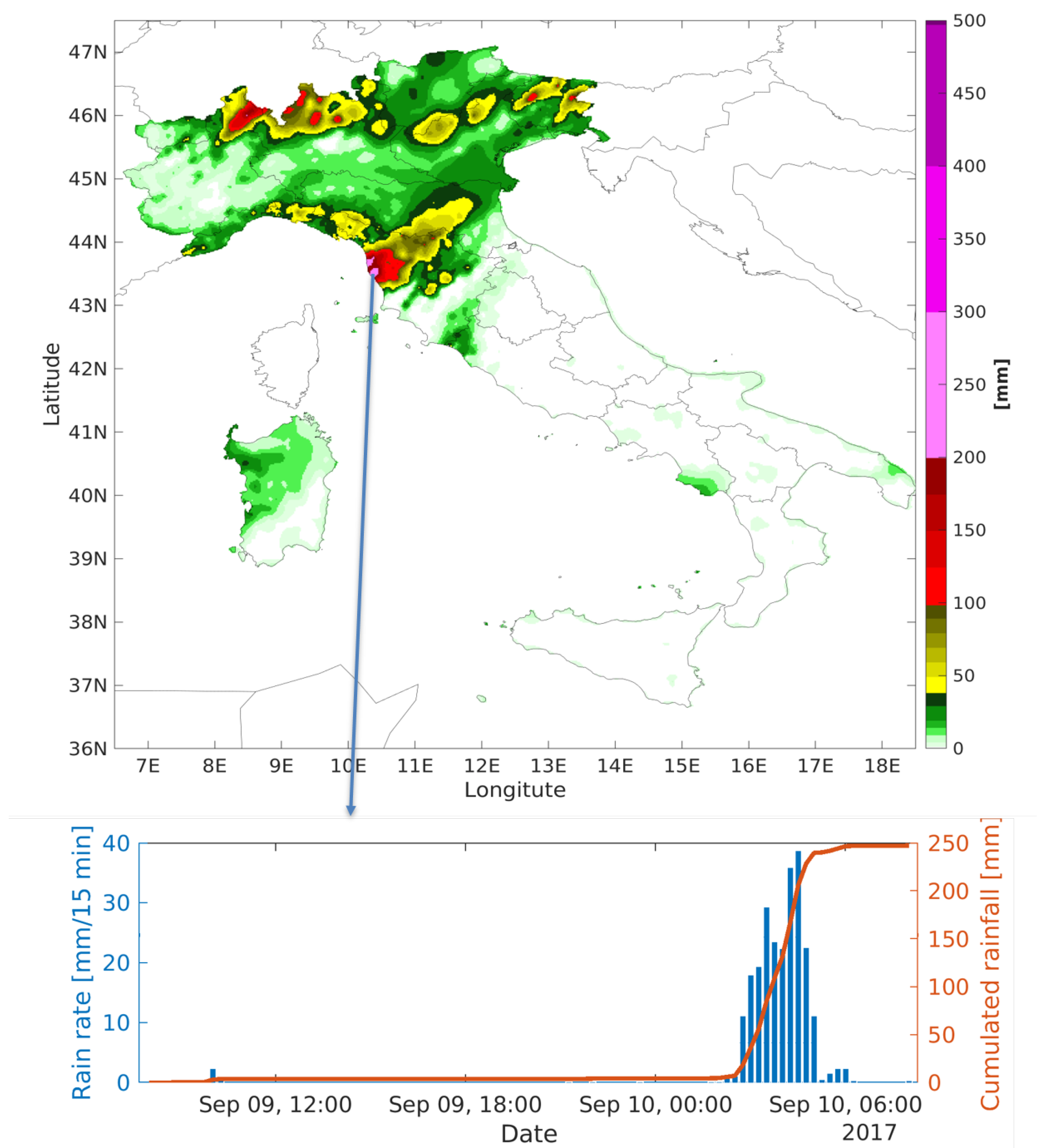
2.1.1. The Livorno Event

The first case study (type II) is the Livorno extreme weather event that took place in the night between 9 and 10 September 2017. Starting from the morning of 9 September a large trough deepened on the western Mediterranean, generating an intense flow of mild and extremely humid air from the South, over all the Tyrrhenian sectors and the eastern part of the Ligurian Sea. From the evening of 9 September, the cold airflow associated with vorticity at 500 hPa was supportive of instability conditions on Tuscany region (not shown).

The environment was also conducive to the development of intense persistent local convective precipitation systems, not only because of the slow evolution of the depression area but also because of the wind shear (not shown).

The resulting observed Quantitative Precipitation Estimate (QPE) for the time period 18UTC 9 September 2017–06UTC 10 September 2017 is shown in Figure 1. The map is obtained interpolating the raingauge data using a semivariogram directly estimated from data themselves [21] (courtesy of the Italian Civil Protection Department). The lower panel of Figure 1 highlight the very timely concentrate rainfall event (Type II) with more than 200 mm of rain felt down in three hours. It was also found that an intense lightning activity, indicative of the ongoing convective dynamics, took place (not shown).

2.1.2. The Silvi Marina Event

The second case study (type I) is the Silvi Marina rainfall event that took place on 14–15 November 2017 in central Italy affecting mainly Abruzzo, Marche and Umbria regions. Around 00UTC on 14 November 2017 an isolated trough at 500 hPa appeared over the Italian peninsula, shrinking and slowly moving towards southern Italy 24 h later. The synoptic scale system advected moist and warm air in the lower troposphere (850 hPa) from Africa towards Apennines mountains range in Central Italy.

The resulting observed QPE map for the 24 h of 15 November 2017 is shown in Figure 2 (courtesy of the Italian Civil Protection Department). The raingauge observation (lower panel in Figure 2) confirm that it is a type I event with a constant rainfall falling for more than 12 h during the day with a 15 min rain rate less than 10 mm.

In this respect, also the number of lightning strokes observed during the two days of the event was negligible (not shown).

2.2. WRF Model Setup

The Weather Research and Forecasting (WRF) model [13] was selected as numerical weather model to accomplish all the experiments carried out within the framework of the STEAM project. It is a compressible non-hydrostatic model with mass-based terrain-following coordinates that was developed at the National Center for Atmospheric Research (NCAR) in collaboration with several institutes and universities for operational weather forecasting and atmospheric science research. In this work the adopted version for WRF is 3.8.1, while for the data assimilation package (WRFDA [22]) is 3.9.1. For this study the three domains setup shown in Figure 3 has been adopted. The domains have, respectively, a horizontal grid spacing of 13.5 (250 × 250 grid points), 4.5 (451 × 450) and 1.5 km (943 × 883) with 50 vertical levels (Figure 3, all domains top reach 50 hPa).

All the simulations are performed with the same set of physical parameterizations, described hereafter, that have already been successfully tested in the study of similar events [19,23,24]. Concerning the surface layer, the MM5 scheme has been adopted [25,26,27]. A convective velocity following [28] is used to enhance surface fluxes of heat and moisture. For the land surface processes, the Rapid Update Cycle (RUC) scheme has a multi-level soil model (6 levels) with higher resolution in the upper soil layer (0, 5, 20, 40, 160, 300 cm) [29,30]. The planetary boundary layer (PBL) dynamics is parameterized with the diagnostic non-local Yonsei University PBL scheme [31]. The WSM6 microphysics six-class scheme is adopted to include graupel and its associated processes [32]. Finally, the radiative processes are parameterized by means of the longwave and shortwave RRTMG schemes [33].

The initial and lateral boundary conditions are derived from NCEP-GFS (National Centers for Environmental Prediction Global Forecast System) analysis and forecast data available at a horizontal grid spacing of 0.25${}^{\circ }$× 0.25${}^{\circ }$ and a time resolution of 3 h, as well as the ECMWF-IFS (European Center for Medium-Range Weather Forecasts Integrated Forecasting System) at a horizontal resolution of 0.125${}^{\circ }$× 0.125${}^{\circ }$ and a time resolution of 3 h.

2.3. Data Assimilation Techniques

The data ingestion was performed according to three different methodologies: direct insertion, a nudging-like technique and 3DVAR assimilation [22,34]. With direct insertion we mean that a given variable in the NWP model is substituted with the corresponding one retrieved by EO sensors. This technique was used with the Sea Surface Temperature (SST) and the Land Surface Temperature (LST). The nudging-like technique was applied for the Soil Moisture (SM) observations and included different steps. Firstly, a difference map between the Sentinel-1-derived SM (re-projected over the WRF grid) and the WRF SM from the first level of soil model (in correspondence with the points observed by Sentinel-1) was produced; then the resulting map was interpolated in the horizontal plane to fill the gaps in the Sentinel-1-derived maps and added to the original WRF SM field in the first (superficial) level. At this point, the new SM field was propagated in the underlying vertical levels by linearly interpolating the difference between the observed and simulated SM assuming a difference equal to 0 in the deepest level. This is done because the Sentinel-1 observation is only superficial and in the deepest layers the value of the model is hypothesized to be more reliable.

Wind speed (WS) and wind direction (WD) from Sentinel-1 and Zenith Total Delay (ZTD) from InSAR and GNSS were assimilated using the 3DVAR technique. In particular, for the GNSS a 3 h cycle technique was implemented to take advantage of the high temporal resolution.The 3 h cycling 3DVAR implies each time the update of the background for the current analysis using the 3 h forecast of the previous cycle. The 3DVAR main purpose is to provide an optimal estimate of the atmospheric state, by minimising the cost function of Equation (1) [35]

$$J\left(x\right)=\frac{1}{2}{\left(\mathbf{x}-{\mathbf{x}}^b\right)}^T{\mathbf{B}}^{-1}\left(\mathbf{x}-{\mathbf{x}}^b\right)+\frac{1}{2}{\left(\mathbf{y}-{\mathbf{y}}^0\right)}^T{\mathbf{R}}^{-1}\left(\mathbf{y}-{\mathbf{y}}^0\right),$$

(1)

where $\mathbf{x}$ is the analysis to be found that minimizes the cost function $J\left(x\right)$, ${\mathbf{x}}^b$ is the first guess of the NWP model, ${\mathbf{y}}^0$ is the assimilated observation and $\mathbf{y}=\mathcal{H}\left(\mathbf{x}\right)$ is the model-derived observation transformed from the analysis $\mathbf{x}$ by the observation operator $\mathcal{H}$ for comparison against ${\mathbf{y}}^0$. The solution of (1) represents an a posteriori maximum likelihood estimate of the true state given two sources of data: the first guess ${\mathbf{x}}^b$ and the observation ${\mathbf{y}}^0$. The analysis fit to this data is weighted by the estimates of their errors, contained in $\mathbf{B}$ and $\mathbf{R}$, which are the background error covariance matrix and the observation error covariance matrix, respectively. The $\mathbf{R}$ matrix is the sum of two distinct error covariance matrices: the observation (instrumental) matrix and the representativity error matrix. This matrix is assumed to be diagonal, as done in most of the models [34] assuming the correlations between different instruments and between different observations made by the same instruments equal to zero.

This work adopts the Control Variable option 5 (CV5) of the WRFDA package for the $\mathbf{B}$ matrix calculation using the National Meteorological Center (NMC) method [36] (for more details refer to WRFDA User Guide ). The NMC method was applied over the entire month of October 2013 with a 24-hour lead time for the forecasts starting at 00:00 UTC and a 12-hour lead time for the ones initialized at 12:00 UTC of the same day. The differences between the two forecasts ($t+24$ and $t+12$) valid for the same reference time were used to calculate the domains specific error statistics.

3. Observational Data Description, Assimilation and Experimental Design

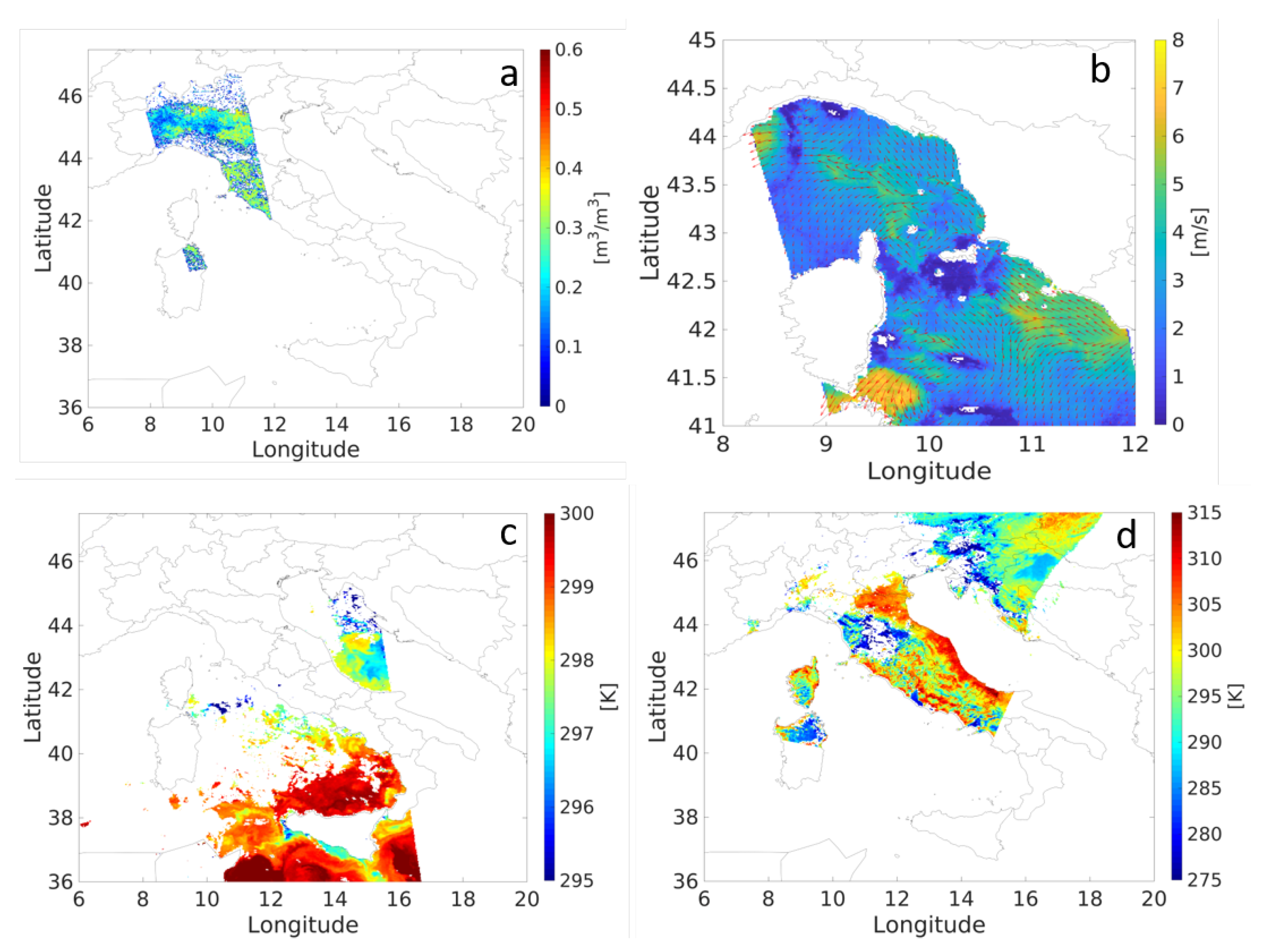
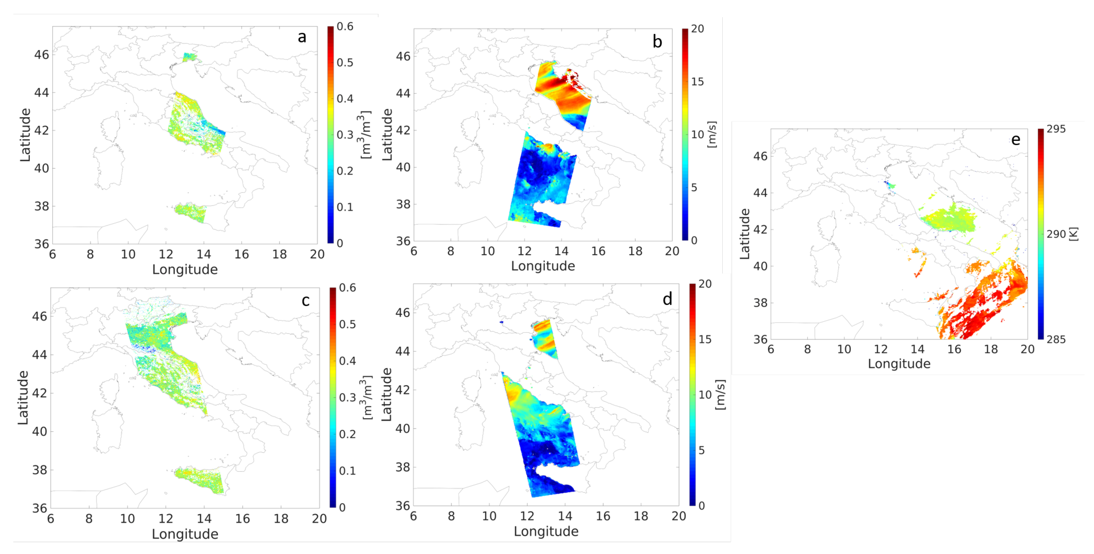
3.1. The EO Variables of Interest

As mentioned in the Introduction, this research focuses on Sentinel-derived and GNSS-derived data. The family of missions called Sentinels were specifically developed for the operational needs of the Copernicus programme. Each mission is based on a constellation of two satellites to ensure that the revisit time (less than 6 days) and the spatial coverage of the data are compliant with the requirements of the programme. In this study, Sentinel-1 and Sentinel-3 data were used. Sentinel-1 is a polar-orbiting, all-weather, day-and-night C-band (5.4 GHz) SAR mission for land and ocean services. Sentinel-3 is a multi-instrument mission to measure sea and land surface temperature, ocean colour and land colour with high-end accuracy and reliability.

For a detailed description of the reasoning behind the selection of the EO variables to be ingested into the WRF model, that was based on the Observing Systems Capability Analysis and Review (OSCAR) tool, the reader is referred to Reference [12]. Through OSCAR, which is a resource developed by World Meteorological Organization (WMO) in support of Earth Observation applications, studies and global coordination (https://www.wmo-sat.info/oscar/), a set of requirements for observation of physical variables in support of WMO programs is available.

By giving priority to the availability of data at high spatial resolution among those indicated by OSCAR as the most relevant for NWP applications, we selected the following variables: ZTD (that can be retrieved using SAR interferometric technique from Sentinel-1 or GNSS data), surface soil moisture and surface wind vector over the sea (that can be retrieved using Sentinel-1 data), sea and land surface temperature (that can be retrieved using Sentinel-3 data). Some of these variables (wind vector, sea and land surface temperature) are directly available as Sentinel products, while others (soil moisture and integrated water vapour) have to be retrieved. A description of the methods used to estimate these variables is provided in the Appendix A and Appendix B.

3.2. GNSS Observations for the Livorno and Silvi Marina Test Cases

ZTD time series at 30 s resolution were estimated for all the geodetic permanent stations within the WRF domain to perform data assimilation experiments. For the selected events the data of 375 permanent stations were available (Figure 4). The iono-free phase range combination of dual-frequency GPS-only observations for three days including the selected events were processed in PPP mode. An accuracy assessment [37] of the GNSS-derived ZTD time series was performed by comparison with 43 radiosonde launches from eight Italian radiosounding datasets. This comparison yielded a mean difference in ZTD of 0.3 cm and a standard deviation of 1.46 cm (not shown).

GNSS ZTDs are used also to validate the retrieved maps of InSAR ZTD in the Silvi Marina test case. The statistics of the differences for this case are reported in

Table 1. InSAR Zenith Total Delay (ZTD) vs. GNSS ZTD–Silvi Marina test case.

	before Orbital Error Removal	after Orbital Error Removal
no. of data	53	53
mean [cm]	1.24	−0.14
standard deviation [cm]	4.87	2.42
min [cm]	−9.54	−5.19
max [cm]	9.89	4.46

. A good agreement is reached between GNSS and InSAR after orbital error removal, with a standard deviation of the residuals in the order of few cm.

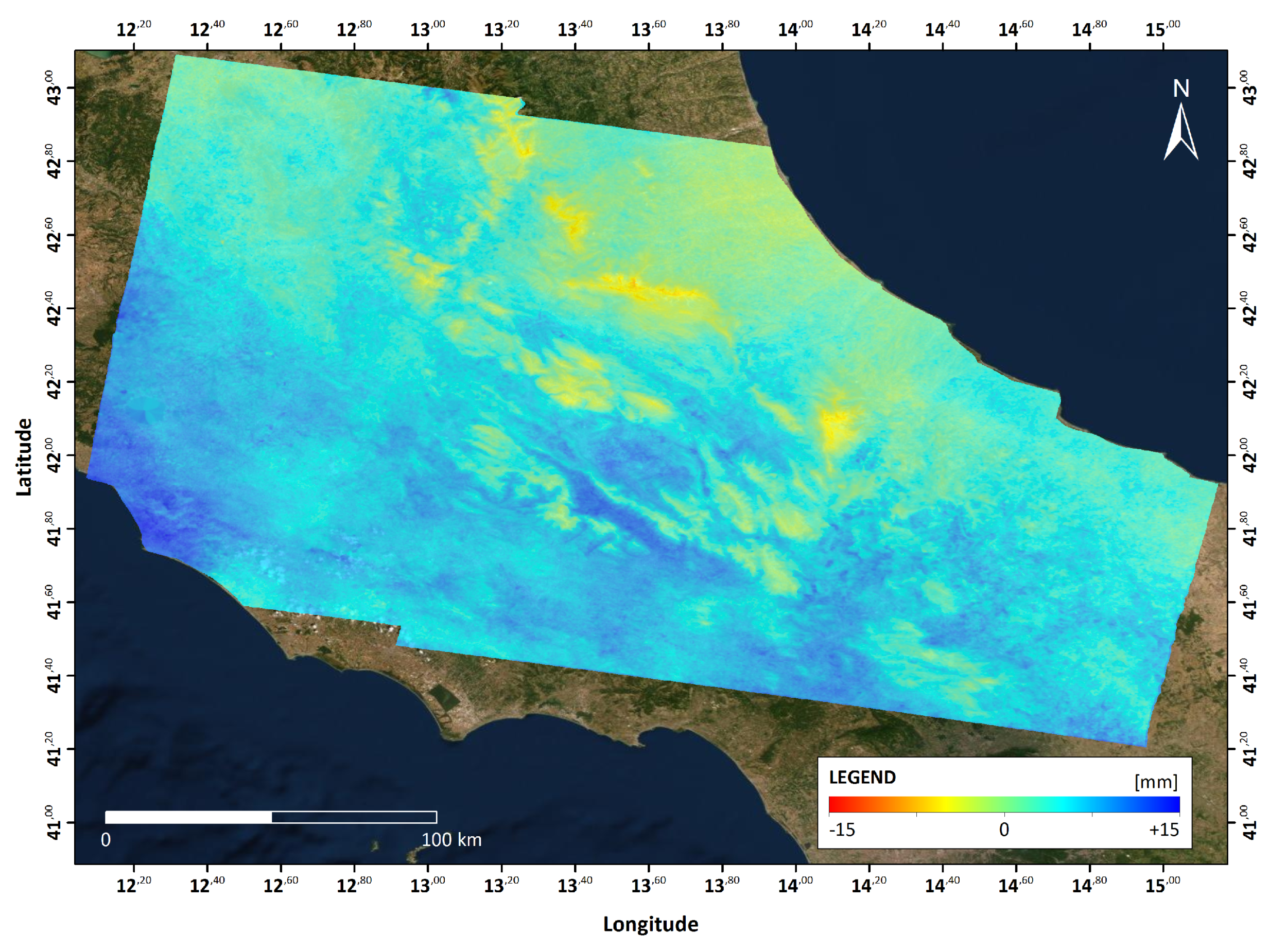
3.3. Sentinel Observations for the Livorno Test Case

The following data were available directly through the Sentinel catalogues: (1) land and sea surface temperatures derived from the Sea and Land Surface Temperature Radiometer (SLSTR) on board of Sentinel-3, generated on a 1 × 1 km${}^2$ grid; (2) wind vector (speed and direction at 10 m a.s.l.) included in the Ocean Wind Field (OWI) component of the Sentinel-1 Level-2 Ocean (OCN) product (again generated on a 1 × 1 km${}^2$ grid). In particular, for the SST, the Sentinel-3 data acquired on 9 September 2017 at 20:36 UTC were gathered, while for LST, the Sentinel-3 data acquired on 9 September 2017 at 09:50 UTC were used. For what concerns SM, WD and WS, Sentinel-1 observed the Livorno area on 8 September 2017 at 17:14 UTC. To apply the multi-temporal SM retrieval algorithm, even the Sentinel-1 data acquired on 2 September, 27 August, 21 August and 15 August 2017 were used. Sentinel-1 ground range detected products were collected to estimate SM; these data were multi-looked (10 × 10), calibrated and geocoded using the 30 m SRTM DEM.

Figure 5 shows the maps of soil moisture (a), wind field (b), sea surface temperature (c) and land surface temperature (d). The SM map shows that the area corresponding to the observed QPE maxima is well captured by the Sentinel-1 data and corresponds to quite high SM values, around 0.3 m${}^3$/m${}^3$. As for the wind field, the map shows that an intense Scirocco wind was blowing along the southern Tuscany and northern Lazio coastline, while the pattern of the wind over the sea in front of northern Tuscany was more disorganized and chaotic. Additionally, an intense wind jet was blowing near the Strait of Bonifacio, between Corsica and Sardinia. The Sentinel-3 derived SST map shows valid values (without cloud coverage) mainly on the southern part of the area of interest around Sicily Island, while not valid observations are available in front of the Tuscany coastlines. The problem of the scarcity of valid observations when severe weather events occur is common for optical data. For what concerns the Sentinel-3 derived LST data, it can be seen that the northern part of Tuscany, near the area mostly affected by the observed torrential rainfall phenomenon, shows a significantly lower LST than the surrounding areas, especially along the Adriatic coastlines and the eastern portion of Pianura Padana.

An inverse square distance weighting interpolation of the Sentinel data on the WRF domains computational grids allowed obtaining the Sentinel maps into to the resolution of the innermost domain (1.5 km) before the assimilation. As mentioned in Section 2.3, the SM maps are also propagated in all the model soil layers (refer to Figure 3 in Reference [12]). Concerning ZTD measurements, for the Livorno test case the ZTD from InSAR was not available, thus only GNSS data were assimilated.

3.4. Sentinel Observations for the Silvi Marina Test Case

For the SST, the Sentinel-3 data acquired on 14 November 2017 at 20:24 UTC were used, while cloud free optical data to derive LST were not found for the Silvi Marina event. For what concerns SM, WD and WS, Sentinel-1 observed the area of interest area on 14 November 2017 at 05:10 UTC (descending orbit) and at 17:06 UTC (ascending orbit). To apply the multi-temporal SM retrieval algorithm, even the Sentinel-1 data acquired on 8 November, 2 November, 27 October and 21 October 2017 were gathered (both ascending and descending orbits). Figure 6 shows the available EO observational data.

Looking at the SM maps, the area corresponding to the observed QPE maxima, over Marche and Abruzzo Apennines is well captured by the Sentinel data and it corresponds to SM values around 0.3 m${}^3$/m${}^3$. The SST map shows valid values only two days ahead the observed event, mainly on the swat southern part on the Ionian Sea, as well as in front of the Abruzzo and Marche coastline.

Also in this case an inverse square distance weighting interpolation of the Sentinel data on the WRF domains computational grids allowed to obtain the Sentinel maps (SM, SST, WIND) at the resolution of the innermost domain (1.5 km) before the assimilation.

For the Silvi Marina case, also ZTD map retrieved from Sentinel-1 is available. In this work 49 Sentinel-1 images have been downloaded and processed by SqueeSAR [38]. Details of the images processed are reported in

Table 2. Details of the images processed for Silvi Marina test case.

Number of Images	49
First Image	18 May 2017
Last Image	14 March 2018
Image Dimensions [pixels]	67,395 × 12,141
AOI [km]	340 × 200

.

Atmospheric products have been subsampled, roughly at 100 × 100 [m${}^2$]. In Figure 7 an example of the derived atmospheric product is given, depicting the Area of Interest (AOI). Along with the Atmospheric Phase Screen (APS) products a digital terrain model of the AOI used in data processing and an incidence angle map have been generated, to allow the data projection along the zenith local direction.

This variable has been further under sampled for the assimilation due to the fact that the original resolution at 100 m increases the computational cost of the simulation and, most importantly, violates the assumption of spatially independent observation errors made in Section 2.3 for the $\mathbf{R}$ matrix [9,10]. For this reason, Reference [10] applied a thinning procedure choosing the nearest available InSAR measurement to each model grid point to obtain a 1 km observed map (same resolution as the inner domain of their setup). With the same method, Reference [9] used a thinning distance of 15 km (for an inner domain resolution of 3 km). To choose the best thinning resolution we performed few sensitivity tests investigating the different observed and modeled ZTD in terms of BIAS and RMSE before and after the assimilation using various InSAR ZTD map resolutions. The thinning resolutions adopted for the sensitivity are 1.5 km, 4.5 km and 13.5 km (the three WRF nested domain grid spacings). For each experiment, the observed point nearest to the center of the corresponding grid cell is kept and the rest is discarded.

Because of the differences between the WRF model orography and the InSAR Digital Elevation Model (DEM), a correction of the ZTD has to be introduced while comparing the WRF ZTD field and the InSAR-derived one. In particular, since the ZTD is the vertical integral of the refractivity N [39], which is a function of the pressure of dry air, the partial pressure of water vapour and the temperature [40,41,42], a simple ZTD correction based on the model variables can be implemented.

Let $Z_{obs}$ be the height of the DEM associated to the ZTD InSAR observation in a specific position. When it is lower than the WRF DEM, $Z_{obs1}<Z_0$, a positive correction using the first model level refractivity $N_1$,

$$\Delta \mathrm{ZTD}={10}^{-6}\left[(Z_0-Z_{obs1})·N_1\right]$$

(2)

is introduced. In case the InSAR DEM is higher than the WRF DEM, a negative correction to the model ZTD has to be applied, namely

$$\Delta \mathrm{ZTD}=-{10}^{-6}\left[\sum _{k=1}^{k_0}(Z_k-Z_{k-1})·N_k+(Z_{obs2}-Z_{k_0})·N_{K_0+1}\right],$$

(3)

where $k_0$ corresponds to the last model level that is below the InSAR DEM, $Z_{obs2}$.

To find the best resolution of the InSAR ZTD to be assimilated, the modeled ZTD calculated on the innermost domain is compared with the InSAR ZTD map resampled on its grid (1.5 km resolution), after the correction due to the height differences between the DEMs described above. The GFS-driven OL (taken as an example) simulation has a BIAS of −0.15 cm and a RMSE value of 2.4 cm with respect to the InSAR ZTD. The simulations assimilating InSAR ZTD at 1.5, 4.5 and 13.5 km resolution have a BIAS of −0.69, −0.27 and −0.35 cm and a RMSE of 1.70, 1.64 and 1.92 cm respectively. Thus, all the simulation assimilating the InSAR ZTD at different resolutions (1.5, 4.5 and 13.5 km) reduce the RMSE but increase the BIAS. Since the RMSE is reduced at most with the assimilation of the InSAR ZTD at 4.5 km resolution, this thinning resolution is chosen for the InSAR assimilation in this case. Future work is planned to estimate the effects on the rain forecast of assimilating the InSAR ZTD maps at different resolutions and with different uncertainties.

3.5. Experimental Design

To comply with the objective of the STEAM project (discussed in the Introduction), for extreme events investigation, it was crucial to choose test cases with Sentinel 1 and 3 observations in a reasonable, considering the satellite revisiting times (6 days for Sentinel 1 (every 6 days over Italy there are two passages, one in the moring and another in the evening) and 1–2 days for Sentinel 3), temporal interval before the event. The available observations that follow this requirement are introduced in Section 3.3 and Section 3.4. Furthermore, to assess the impact on the forecast of each satellites product it was essential to perform a set of experiment assimilating one variable at a time and afterwards one or more experiments assimilating a combination of the most influencing variables. This produced a set of 7 to 9 experiments (for Silvi Marina and Livorno test case respectively).

Table 3. List of experiments, timing and techniques applied for data assimilation for the Livorno and Silvi Marina use cases.

Livorno Use Case
Experiment Name	Assimilated Variable	Assimilation Methodology	Timing (HH UTC DD/MM/YYYY)
OL	-	No assimilation
LST	Land Surface Temperature	Direct insertion	10 UTC 09/09/2017
SST	Sea Surface Temperature	Direct insertion	21 UTC 09/09/2017
SM	Soil Moisture	Nudging-like	18 UTC 08/09/2017
ZTD_GNSS3h	Zenith Total Delay	3DVAR of all obs. available in the time window (1/2 h) around the analysis time	3 h cycling
ZTD_GNSS3h_1ist	Zenith Total Delay	3DVAR only of obs. closest to the analysis time	3 h cycling
WIND	Wind speed and direction	3DVAR	18 UTC 08/09/2017
WIND+SM+ZTD_GNSS3h_1ist	Wind speed and direction, Soil Moisture, Zenith Total Delay	Nudging-like, 3DVAR	Refer to the single variable timing
WIND+SM+ZTD_GNSS3h_1ist_18UTC	Wind speed and direction, Soil Moisture, Zenith Total Delay	Nudging-like, 3DVAR only of obs. closest to the analysis time	18 UTC 08/09/2017
Silvi Marina Use Case
Experiment name	Assimilated Variable	Assimilation Methodology	Timing (HH UTC DD/MM/YYYY)
OL	-	No assimilation
SST	Sea Surface Temperature	Direct insertion	00 UTC 14/11/2017
SM	Soil Moisture	Nudging-like	05 UTC and 17UTC 14/11/2017
ZTD_GNSS3h_1ist	Zenith Total Delay	3DVAR only of obs. closest to the analysis time	3-h cycling
ZTD_INSAR	Zenith Total Delay	3DVAR	05 UTC 14/11/2017
WIND	Wind speed and direction	3DVAR	05 UTC and 17UTC UTC 14/11/2017
WIND+SM+ZTD_INSAR_GNSS3h_1ist	Wind speed and direction, Soil Moisture, Zenith Total Delay	Nudging-like, 3DVAR	05 UTC 14/11/2017

summarizes the experiments methodology, data assimilated (alone or their combinations) and timing for the two use cases. To further consider also the assimilation response to different initialization each set of experiments is performed with two different Global Circulation Models (GCM) namely IFS and GFS. Consequently, for each use case 14 to 18 (for Silvi Marina and Livorno use case respectively) numerical weather modeling experiments were investigated for a total of 32.

Table 3 third column summarize the assimilation technique used for each experiment. The main reason of using different assimilation technique deal with the STEAM project aim. For each EO derived variable the most suitable way of assimilation is chosen to assess the impact of Sentinel satellites products assimilation. It was necessary above all to take into account their revisiting time. Furthermore, another important aspect to deal with is the observation type available from Sentinel, how it is modeled and evolved by the WRF model and what was already available in the WRFDA suite for each type of observation assimilation. Thus, concerning wind field and Zenith Total Delay, the 3dvar technique was chosen among the available assimilation technique because it allows both an assimilation to update initial condition when the observation is available only at a given time (i.e., SM for Livorno use case) and a cycling assimilation technique when observations are available with higher temporal resolution (i.e., ZTD from GNSS). Concerning sea surface temperature and land surface temperature, they are boundary observations, so they were ingested through a direct insertion technique. Finally, the soil moisture is again a boundary condition evolved in time by the model with a 1D (vertical) soil model discretized in 6 vertical levels. Thus, it was assimilated with a nudging-like (it doesn’t take into account model and observation weights, refer to Section 2.3 for the details).

As it is possible to see from Table 3 the two use cases have slightly different experiments. One of the reason is linked to the absence of LST observation for the Silvi Marina use case and of InSAR ZTD for the Livorno one. While, another different is in the ZTD from GNSS assimilation: for the Silvi Marina use cases only one of the two metodologies applied in the Livorno case is implemented because it was the best experiment setup the Livorno use case and it is also the most compliant one with the R matrix assumption of uncorrelated observation (see Section 2.3).

The Livorno case study is initialized at 18 UTC on 8 September 2017, while the Silvi Marina one is initialized at 00 UTC on 14 November 2017. Both use cases have a 3 h update of the boundary conditions and a 48 h forecasting time interval.

4. Validation and Results

To validate all the modeling experiments and identify the best performing WRF setup for each case study, the Method for Object-Based Evaluation [43,44] [MODE] is applied by comparing the Quantitative Precipitation Forecast (QPF) of WRF with the raingauges QPE. MODE identifies precipitation structures in both forecast and observed fields and performs a spatial evaluation of the model capability of reproducing the identified observed objects. Such validation method overcomes the so-called “double-penalty” issue [45], that traditional verification methods suffer from. This is particularly true when comparing high-resolution observational data analysis and cloud-resolving meteorological forecasts in case of deep moist convective and highly localized phenomena. Since traditional methods cannot provide a measure of spatial and temporal match between the forecast and the observed rainfall patterns, it is preferable to use feature-based verification techniques, such as MODE. In this paper 13 different indices provided by MODE validation are considered. They include both pairs of objects attributes and classical statistical scores: centroid distance, angle difference, area ratio, symmetric difference and percentile intensity (in this work above the 90th percentile threshold), Frequency BIAS (FBIAS), Probability of Detection Yes (PODY), False Alarm Ratio (FAR), Critical Success Index (CSI), Hanssen and Kuipers discriminant (HK), Heidke Skill Score (HSS). For a complete description of the indices refer to References [23,24]. The setup of all MODE parameters (except the rainfall threshold) is taken as it is by default. This means that in this work it is used a convolution radius of 1 grid square and a merging threshold above or equal to 1.25.

The main goal of this meteorological validation, from a QPF standpoint, is to select the best meteorological forecast out of the whole set of the sensitivity experiments performed to investigate the impact of assimilating Sentinel and GNSS derived products. The outputs of the MODE validation tool are calculated for three different rainfall thresholds, namely 24, 48 and 72 mm. The evaluation metrics to assess the most reliable meteorological forecast in each set of experiments is performed as in Reference [23]: all the indices and statistical scores described above are calculated for each sensitivity experiment, then the times in which a simulation has been the best for each score is counted. Finally, the simulation ranking as the best for the highest number of times is identified.

Additionally, the behavior of the experiments performed is discussed in the following sections both in terms of spatial indices and in terms of cumulated rainfall thresholds, to infer as many physical insights as possible. For a given experiment or a given index, the MODE spatial indices are compared to the OL ones to see if the assimilation has a positive impact on the forecast. The most relevant results are then highlighted and explained on a physical basis. This twofold approach (number of best scores and discussion on the indices with respect to the OL) is suggested as an alternative to the standard MODE approach [43,44]. This is done because, in its original formulation, MODE makes use of an interest function that depends on a certain number of parameters that are not simple to define. Thus, to avoid extracting partial or wrong information, we decided to follow our simple and physically-oriented approach, as in References [12,24].

4.1. Livorno Test Case

Figure 8 and Figure 9 summarize the QPF values provided by the different modelling experiments for the 12 h time period from 18UTC on 9 September 2017 to 06UTC on 10 September 2017. Figure 8 refers to GFS-driven cases, while Figure 9 refers to IFS-driven cases. The MODE analysis results for the three different thresholds are reported in

Table A2. Spatial and statistical indices calculated through MODE (24 mm rainfall depth threshold) to evaluate the sensitivity forecasts (driven by GFS and IFS respectively) with respect to the Open Loop run for the time interval 18UTC 09/09/2017–06UTC 10/09/2017. The best performance for each score is highlighted in bold.

24 mm (GFS) Livorno Use Case
Run	CENTROID DIST	ANGLE DIFF	AREA RATIO	SYMMETRIC DIFF	INTERSECTION AREA	UNION AREA	P90 RATIO	FBIAS	PODY	FAR	CSI	HK	HSS
OL	5.34	4.15	0.73	3027.00	3395.00	6422.00	0.95	0.86	0.59	0.31	0.47	0.48	0.50
LST	5.88	23.10	0.70	3440.00	3202.00	6642.00	0.93	0.82	0.54	0.34	0.43	0.43	0.46
SM	4.73	12.86	0.72	3536.00	3209.00	6745.00	0.93	0.77	0.55	0.29	0.45	0.46	0.49
SST	4.97	5.64	0.73	2959.00	3450.00	6409.00	0.92	0.88	0.60	0.32	0.47	0.48	0.50
WIND	7.63	7.50	0.79	3902.00	3228.00	7130.00	0.88	0.92	0.55	0.40	0.41	0.40	0.41
WIND+SM+ZTD_GNSS3h_1ist	9.44	8.17	0.83	3683.00	3470.00	7153.00	0.98	0.93	0.59	0.37	0.44	0.45	0.46
WIND+SM+ZTD_GNSS3h_1ist_18UTC	14.09	12.80	0.78	3411.00	3429.00	6840.00	0.82	0.91	0.58	0.36	0.44	0.45	0.46
ZTD_GNSS3h	6.58	22.54	0.76	4019.00	3067.00	7086.00	0.95	1.07	0.52	0.51	0.34	0.30	0.29
ZTD_GNSS3h_1ist	7.70	2.89	0.80	3741.00	3329.00	7070.00	0.92	0.88	0.57	0.36	0.43	0.44	0.45
	Best small	Best small	Best = 1	Best small	Best big	Best small	Best = 1	Best = 1	Best = 1	Best = 0	Best = 1	Best = 1	Best = 1
24 mm (IFS) Livorno Use Case
Run	CENTROID DIST	ANGLE DIFF	AREA RATIO	SYMMETRIC DIFF	INTERSECTION AREA	UNION AREA	P90 RATIO	FBIAS	PODY	FAR	CSI	HK	HSS
OL	18.77	65.31	0.76	3323.00	3418.00	6741.00	0.96	0.77	0.59	0.24	0.50	0.51	0.55
LST	15.33	40.81	0.70	3484.00	3192.00	6676.00	0.96	0.80	0.54	0.32	0.43	0.44	0.47
SM	16.99	50.12	0.77	3474.00	3295.00	6769.00	0.97	0.82	0.57	0.31	0.46	0.47	0.50
SST	15.88	47.68	0.76	3152.00	3434.00	6586.00	0.94	0.80	0.59	0.26	0.49	0.51	0.54
WIND	11.28	40.31	0.56	3105.00	2875.00	5980.00	0.82	0.69	0.50	0.27	0.43	0.43	0.47
WIND+SM+ZTD_GNSS3h_1ist	16.52	10.32	0.66	3985.00	2875.00	6860.00	0.98	0.78	0.49	0.37	0.38	0.37	0.40
WIND+SM+ZTD_GNSS3h_1ist_18UTC	11.52	24.46	0.62	3234.00	3138.00	6372.00	0.91	0.66	0.53	0.19	0.48	0.48	0.54
ZTD_GNSS3h	24.91	2.59	0.95	5522.00	3271.00	8793.00	0.93	1.09	0.56	0.49	0.36	0.34	0.33
ZTD_GNSS3h_1ist	10.65	14.09	0.73	4058.00	2961.00	7019.00	0.98	0.75	0.50	0.32	0.41	0.40	0.44
	Best small	Best small	Best = 1	Best small	Best big	Best small	Best = 1	Best = 1	Best = 1	Best = 0	Best = 1	Best = 1	Best = 1

(24 mm),

Table A3. Spatial and statistical indices calculated through MODE (48 mm rainfall depth threshold) to evaluate the sensitivity forecasts (driven by GFS and IFS respectively) with respect to the Open Loop run for the time interval 18UTC 09/09/2017–06UTC 10/09/2017. The best performance for each score is highlighted in bold.

48 mm (GFS) Livorno Use Case
Run	CENTROID DIST	ANGLE DIFF	AREA RATIO	SYMMETRIC DIFF	INTERSECTION AREA	UNION AREA	P90 RATIO	FBIAS	PODY	FAR	CSI	HK	HSS
OL	6.93	12.37	0.58	1653.00	760.00	2413.00	0.97	0.68	0.37	0.46	0.28	0.33	0.39
LST	7.07	21.42	0.67	1225.00	987.00	2212.00	0.90	0.81	0.48	0.40	0.36	0.45	0.49
SM	9.95	21.70	0.61	1456.00	817.00	2273.00	0.96	0.62	0.41	0.35	0.33	0.38	0.46
SST	8.09	23.04	0.63	1623.00	750.00	2373.00	0.92	0.65	0.36	0.44	0.28	0.33	0.39
WIND	3.80	28.05	0.98	1833.00	1022.00	2855.00	0.99	1.08	0.50	0.54	0.31	0.43	0.42
WIND+SM+ZTD_GNSS3h_1ist	6.68	25.38	0.98	1325.00	1276.00	2601.00	0.98	1.06	0.62	0.41	0.43	0.57	0.56
WIND+SM+ZTD_GNSS3h_1ist_18UTC	5.78	13.95	0.89	1256.00	1410.00	2666.00	0.87	1.22	0.69	0.44	0.45	0.63	0.57
ZTD_GNSS3h	30.67	2.35	0.69	1629.00	809.00	2438.00	0.99	1.18	0.43	0.64	0.24	0.34	0.32
ZTD_GNSS3h_1ist	29.33	2.38	0.80	2042.00	700.00	2742.00	0.95	0.91	0.35	0.62	0.22	0.28	0.30
	Best small	Best small	Best = 1	Best small	Best big	Best small	Best = 1	Best = 1	Best = 1	Best = 0	Best = 1	Best = 1	Best = 1
48 mm (IFS) Livorno Use Case
Run	CENTROID DIST	ANGLE DIFF	AREA RATIO	SYMMETRIC DIFF	INTERSECTION AREA	UNION AREA	P90 RATIO	FBIAS	PODY	FAR	CSI	HK	HSS
OL	13.39	80.17	0.44	1731.00	537.00	2268.00	0.74	0.67	0.29	0.57	0.21	0.25	0.29
LST	7.06	13.13	0.30	1354.00	570.00	1924.00	0.75	0.59	0.32	0.46	0.25	0.29	0.35
SM	23.40	41.72	0.31	2147.00	186.00	2333.00	0.98	0.62	0.14	0.78	0.09	0.08	0.10
SST	8.41	48.21	0.53	1873.00	533.00	2406.00	0.73	0.67	0.30	0.56	0.21	0.25	0.30
WIND	1.19	18.00	0.76	1171.00	1105.00	2276.00	0.92	0.88	0.56	0.36	0.43	0.53	0.56
WIND+SM+ZTD_GNSS3h_1ist	6.78	8.92	0.47	1226.00	795.00	2021.00	0.98	0.56	0.41	0.27	0.36	0.39	0.49
WIND+SM+ZTD_GNSS3h_1ist_18UTC	6.99	16.59	0.72	1040.00	1130.00	2170.00	0.92	0.81	0.56	0.31	0.45	0.53	0.58
ZTD_GNSS3h	12.97	19.91	0.49	1757.00	550.00	2307.00	0.83	1.13	0.30	0.74	0.16	0.20	0.19
ZTD_GNSS3h_1ist	13.91	41.69	0.58	1812.00	685.00	2497.00	0.93	0.75	0.33	0.56	0.24	0.29	0.32
	Best small	Best small	Best = 1	Best small	Best big	Best small	Best = 1	Best = 1	Best = 1	Best = 0	Best = 1	Best = 1	Best = 1

(48 mm) and

Table A4. Spatial and statistical indices calculated through MODE (72 mm rainfall depth threshold) to evaluate the sensitivity forecasts (driven by GFS and IFS respectively) with respect to the Open Loop run for the time interval 18UTC 09/09/2017–06UTC 10/09/2017. The best performance for each score is highlighted in bold.

72 mm (GFS) Livorno Use Case
Run	CENTROID DIST	ANGLE DIFF	AREA RATIO	SYMMETRIC DIFF	INTERSECTION AREA	UNION AREA	P90 RATIO	FBIAS	PODY	FAR	CSI	HK	HSS
OL	12.32	9.93	0.54	1201.00	227.00	1428.00	0.97	0.55	0.21	0.61	0.16	0.19	0.25
LST	11.47	20.60	0.53	1118.00	263.00	1381.00	0.92	0.61	0.25	0.59	0.18	0.23	0.28
SM	11.57	20.55	0.64	1115.00	322.00	1437.00	0.93	0.65	0.30	0.53	0.23	0.28	0.34
SST	12.52	10.44	0.54	1213.00	221.00	1434.00	0.96	0.55	0.21	0.62	0.15	0.19	0.24
WIND	11.49	15.39	0.66	1078.00	352.00	1430.00	0.97	1.06	0.33	0.69	0.19	0.29	0.28
WIND+SM+ZTD_GNSS3h_1ist	9.11	13.49	0.78	755.00	577.00	1332.00	0.95	1.06	0.54	0.49	0.36	0.51	0.50
WIND+SM+ZTD_GNSS3h_1ist_18UTC	11.50	22.88	0.71	1217.00	681.00	1898.00	0.97	1.53	0.64	0.58	0.34	0.59	0.47
ZTD_GNSS3h	38.14	2.82	0.70	1298.00	262.00	1560.00	0.95	0.84	0.25	0.71	0.15	0.21	0.23
ZTD_GNSS3h_1ist	20.16	0.06	0.68	1317.00	242.00	1559.00	0.90	0.71	0.23	0.68	0.15	0.20	0.23
	Best small	Best small	Best = 1	Best small	Best big	Best small	Best = 1	Best = 1	Best = 1	Best = 0	Best = 1	Best = 1	Best = 1
72 mm (IFS) Livorno Use Case
Run	CENTROID DIST	ANGLE DIFF	AREA RATIO	SYMMETRIC DIFF	INTERSECTION AREA	UNION AREA	P90 RATIO	FBIAS	PODY	FAR	CSI	HK	HSS
OL	14.53	0.84	0.09	973.00	99.00	1072.00	0.87	0.23	0.09	0.60	0.08	0.09	0.13
LST	12.49	13.28	0.05	1021.00	51.00	1072.00	0.82	0.29	0.05	0.83	0.04	0.03	0.05
SM	16.38	4.69	0.04	1031.00	41.00	1072.00	0.85	0.48	0.04	0.92	0.03	0.01	0.02
SST	15.03	1.67	0.08	989.00	84.00	1073.00	0.85	0.21	0.08	0.62	0.07	0.07	0.12
WIND	8.37	0.94	0.62	783.00	477.00	1260.00	0.93	0.73	0.45	0.38	0.35	0.43	0.50
WIND+SM+ZTD_GNSS3h_1ist	11.23	6.73	0.49	914.00	344.00	1258.00	0.98	0.51	0.32	0.36	0.27	0.31	0.41
WIND+SM+ZTD_GNSS3h_1ist_18UTC	9.82	21.93	0.58	996.00	348.00	1344.00	0.87	0.63	0.33	0.48	0.25	0.31	0.38
ZTD_GNSS3h	16.77	19.09	0.33	1371.00	30.00	1401.00	0.99	0.70	0.03	0.96	0.02	-0.01	-0.01
ZTD_GNSS3h_1ist	8.10	3.48	0.25	872.00	233.00	1105.00	0.91	0.48	0.22	0.54	0.17	0.21	0.27
	Best small	Best small	Best = 1	Best small	Best big	Best small	Best = 1	Best = 1	Best = 1	Best = 0	Best = 1	Best = 1	Best = 1

(72 mm). In the case of the GFS-driven experiments, the best performing run is WIND+SM+ZTD_GNSS3h_1ist (3DVAR wind at the analysis time, SM assimilation at the analysis time, 3DVAR 3h cycling with the 1-minute ZTD observations temporally nearest to the analysis time) with a total of 15 best scores (

Table A5. Summary of the sensitivity performances (GFS-driven cases). The times in which each forecast has the best result for each score is counted for each threshold and summarized in a total count (summing Table A2, Table A3 and Table A4) that is used to find the best simulation.

Livorno Use Case
24 mm	48 mm	72 mm	TOT	GFS-driven CASES
3	0	1	4	OL
0	2	0	2	LST
2	0	0	2	SM
5	0	0	5	SST
0	3	2	5	WIND
4	3	8	15	WIND+SM+ZTD_GNSS3h_1ist
0	5	4	9	WIND+SM+ZTD_GNSS3h_1ist_18UTC
1	1	0	2	ZTD_GNSS3h
1	0	1	2	ZTD_GNSS3h_1ist

and

Table A6. Summary of the sensitivity performances (IFS-driven cases). The times in which each forecast has the best result for each score is counted for each threshold and summarized in a total count (summing Table A2, Table A3 and Table A4) that is used to find the best simulation.

Livorno Use Case
24 mm	48 mm	72 mm	TOT	GFS-driven CASES
4	0	2	6	OL
0	1	1	2	LST
0	1	1	2	SM
3	0	0	3	SST
3	5	8	16	WIND
1	3	1	5	WIND+SM+ZTD_GNSS3h_1ist
1	6	0	7	WIND+SM+ZTD_GNSS3h_1ist_18UTC
3	0	1	4	ZTD_GNSS3h
1	0	1	2	ZTD_GNSS3h_1ist

). Conversely, in the case of the IFS-driven experiments, the best performing one is WIND (3DVAR at the analysis time, namely 18 UTC on 08 September 2018), with a total of 16 best scores.

Looking at the different rain depth threshold values, the behaviour of the assimilation of different variables can be discussed. For example, the assimilation of SST performs well at the lowest threshold, which is in line with the findings that the average SST controls the larger scale precipitation [46,47,48]. In fact, these works show that a good representation of the SST is important for a good precipitation forecast, indicating, in particular, that the average SST in the area near the convective event controls the total amount of rain (the warmer the sea, the higher the volume of rain). Other recent works, such as Reference [49], show that the small scales in the SST field may affect the surface wind response and, thus, the formation of convergence lines, that can drive upward motion and precipitation [50]. One of the reason why the SST experiments do not show good performances at the high rain intensity might be the fact that SST is retrieved from Sentinel-3 observations in the optical bands. This means that the presence of clouds limits the extent of the observed area, especially in the vicinity of the convective activity. For the higher thresholds, thus, the assimilation of the SST does not produce positive results, probably because of the lack of fine spatial structure in the SST field near the convective activity.

Assimilating the wind field shows very good values of the maximum rainfall values and gets better and better the higher value of the threshold, meaning that the dynamical features are of crucial importance to model the rain peaks. Also the location of the rainfall area gets more realistic, both in terms of mean position and in terms of extent, with respect to the OL when assimilating the wind field.

Assimilating the ZTD only seems to improve the orientation of the rainfall area consistently through the cases analyzed. This is probably related to a more correct spatial distribution of the water vapor field with respect to the OL case. Moreover, an improvement in the maximum rainfall values and in the extent of the rainfall area is observed, also at the higher thresholds.

Among the runs that assimilate only one variable, SST has the highest number of best scores for the low threshold, WIND has the highest number of best scores for the two higher thresholds with GFS; instead, with IFS, the OL has the highest number of best scores for 24 mm and WIND dominates for 48 mm and 72 mm: this confirms the importance of the wind structure in the simulation of an intense rain event.

The rather heterogeneous response to the assimilated Sentinel and GNSS derived variables by the GFS and IFS-driven experiments is most probably due to the difference in their respective initial conditions fields. For example, Figure 10 represents the difference map between the IFS-driven SM experiment and the Sentinel-derived SM (SM${}_{\mathrm{IFS}}$-SM${}_{\mathrm{S}1}$, on the right) compared to the difference between the GFS-driven SM experiment and the Sentinel-derived SM (SM${}_{\mathrm{GFS}}$-SM${}_{\mathrm{S}1}$, on the left). Furthermore, the SM mean value over the Area Of Interest (AOI) hit by the event has been calculated for the IFS and GFS driven experiments and the Sentinel observation. It is possible to see that the average SM observed by Sentinel over the AOI is closer to the IFS-driven case values with respect to the GFS ones. In fact, Figure 10 reveals bigger differences in the SM${}_{\mathrm{GFS}}$-SM${}_{\mathrm{S}1}$ picture (on the left) with respect to the SM${}_{\mathrm{IFS}}$-SM${}_{\mathrm{S}1}$ one (on the right). This means that the assimilation in the GFS experiment produced a larger change with respect to the assimilation in the IFS one, leading to a bigger impact on the forecast. It is also worth noticing that the assimilation of wind, soil moisture and ZTD all together ranks well for both driving Global Circulation Models (GCMs). Thus, for operational purposes, this can be a recommended assimilation setup possibly with a 3-h cycling 3DVAR because this setup allowed to obtain an improvement both in the timing and the intensity of the rainfall peaks, as highlighted in Reference [12] for the GFS-driven experiment.

To gain a deeper insight of the modelling experiments, the best performing IFS-driven case, namely the WIND one, is compared with the OL. In particular, Figure 11 shows the atmospheric state of the two experiments at 02UTC on 10 September 2017, corresponding to the most intense phase of the observed event, displayed with the VAPOR (Visualization and Analysis Platform for Ocean, Atmosphere and Solar Researchers, www.vapor.ucar.edu) software. Over the same scene (Figure 11), 3D isosurfaces ($5\times {10}^{-5}$ kg/kg) for the rainwater, snow and graupel variables have been rendered in combination with the wind field at 10 m in case of the OL (panel a) and IFS 3DVAR-WIND case (panel c). The results show that over the area interested by the most intense observed rainfall phenomena (blue circle) the OL run is not able to produce any significant convective phenomena, while the IFS 3DVAR-WIND does so. This is also visible in the vertical cross sections of the reflectivity field for the two modelling experiments (green circles panels b and d): while reflectivity is nearly absent nearby the Tuscany coastlines (Livorno area) for the OL experiment (panel b), conversely strong activity is apparent in panel d over the Livorno area and downshear the main convective system, with values peaking up to 50–55 dBz. Similar improvement is achieved also in the GFS-driven case, as shown in Reference [12].

To better understand the impacts of the wind assimilation, the instantaneous 10 m wind field during the intense phase of the event is shown in Figure 12. It is important to notice that one of the most important ingredients responsible of the triggering of this kind of highly-precipitating back-building Mesoscale Convective System (MCS) is the persistence and intensity of the convergence line over the sea in the area in front of the coast hit by the event [19]. Figure 12 shows that IFS OL is not able to produce a significant convective phenomenon over the area hit by the event, because the convergence line over the sea is shifted to the South with respect to the real location for the entire event duration. Conversely, IFS WIND assimilation is able to produce a stronger convergence line with better localization and persistence. Concerning the comparison between IFS and GFS OL simulations, both OL are not able to produce a significant convergence line in the correct position. Furthermore, GFS OL simulation started at 01 UTC to develop a convergence line in front of the Livorno coastline but it rapidly disappeared just one hour later. Instead, the GFS WIND simulation achieved better performance with the presence of the convergence line during the whole event.

4.2. Silvi Marina Test Case

Figure 13 and Figure 14 summarize the QPF values of the different experiments for the 24 h time period from 00UTC on 15 November 2017 to 00UTC on 16 November 2017. Figure 13 refers to the GFS-driven cases, while Figure 14 refers to the IFS-driven ones. The MODE analysis results for the three different thresholds are reported in

Table A7. Spatial and statistical indices calculated through MODE (24 mm rainfall depth threshold) to evaluate the sensitivity forecasts (driven by GFS and IFS respectively) with respect to the Open Loop run for the time interval 00UTC 15/11/2017–00UTC 16/11/2017. The best performance for each score is highlighted in bold.

24 mm (GFS) Silvi Marina Use Case
Run	CENTROID DIST	ANGLE DIFF	AREA RATIO	SYMMETRIC DIFF	INTERSECTION AREA	UNION AREA	P90 RATIO	FBIAS	PODY	FAR	CSI	HK	HSS
OL	10.55	5.70	0.87	2534.00	3533.00	6067.00	0.81	0.91	0.72	0.21	0.60	0.65	0.67
SM	8.78	4.12	0.95	2246.00	3891.00	6137.00	0.84	1.01	0.79	0.22	0.65	0.71	0.71
SST	12.29	5.04	0.95	2322.00	3833.00	6155.00	0.86	0.99	0.78	0.21	0.64	0.71	0.71
WIND	9.05	2.58	0.99	2333.00	3989.00	6322.00	0.89	1.06	0.81	0.24	0.65	0.72	0.71
ZTD_GNSS3h_1ist	11.03	4.70	0.95	1874.00	4342.00	6216.00	0.96	1.13	0.88	0.22	0.71	0.80	0.76
ZTD_INSAR	15.24	5.18	0.99	2143.00	4026.00	6169.00	0.86	1.04	0.82	0.21	0.67	0.74	0.73
WIND+SM+ZTD_INSAR_GNSS3h_1ist	12.44	5.25	0.91	2275.00	3758.00	6033.00	0.85	0.96	0.76	0.21	0.64	0.69	0.70
	Best small	Best small	Best = 1	Best small	Best big	Best small	Best = 1	Best = 1	Best = 1	Best = 0	Best = 1	Best = 1	Best = 1
24mm (IFS) Silvi Marina Use Case
Run	CENTROID DIST	ANGLE DIFF	AREA RATIO	SYMMETRIC DIFF	INTERSECTION AREA	UNION AREA	P90 RATIO	FBIAS	PODY	FAR	CSI	HK	HSS
OL	12.85	6.96	0.86	3068.00	3250.00	6318.00	0.77	0.90	0.66	0.27	0.53	0.58	0.59
SM	12.40	6.78	0.85	3051.00	3226.00	6277.00	0.74	0.90	0.65	0.27	0.53	0.57	0.59
SST	5.88	6.03	0.90	3326.00	3212.00	6538.00	0.80	0.95	0.65	0.31	0.50	0.55	0.56
WIND	12.22	5.44	0.89	2733.00	3488.00	6221.00	0.86	0.96	0.71	0.26	0.57	0.62	0.63
ZTD_GNSS3h_1ist	9.11	2.01	0.90	2857.00	3985.00	6842.00	0.89	1.17	0.81	0.31	0.60	0.68	0.65
ZTD_INSAR	7.03	7.30	0.93	3030.00	3449.00	6479.00	0.81	0.98	0.70	0.29	0.55	0.60	0.61
WIND+SM+ZTD_INSAR_GNSS3h_1ist	11.90	5.54	0.83	3171.00	3124.00	6295.00	0.74	0.88	0.63	0.28	0.51	0.55	0.57
	Best small	Best small	Best = 1	Best small	Best big	Best small	Best = 1	Best = 1	Best = 1	Best = 0	Best = 1	Best = 1	Best = 1

(24 mm),

Table A8. Spatial and statistical indices calculated through MODE (48 mm rainfall depth threshold) to evaluate the sensitivity forecasts (driven by GFS and IFS respectively) with respect to the Open Loop run for the time interval 00UTC 15/11/2017–00UTC 16/11/2017. The best performance for each score is highlighted in bold.

48 mm (GFS) Silvi Marina Use Case
Run	CENTROID DIST	ANGLE DIFF	AREA RATIO	SYMMETRIC DIFF	INTERSECTION AREA	UNION AREA	P90 RATIO	FBIAS	PODY	FAR	CSI	HK	HSS
OL	10.87	14.91	0.53	1775.00	1401.00	3176.00	0.75	0.60	0.48	0.20	0.43	0.46	0.55
SM	10.50	11.80	0.59	1649.00	1567.00	3216.00	0.82	0.70	0.54	0.23	0.47	0.51	0.58
SST	11.89	12.09	0.60	1790.00	1499.00	3289.00	0.82	0.74	0.52	0.31	0.42	0.47	0.53
WIND	8.33	9.53	0.65	1724.00	1613.00	3337.00	0.88	0.84	0.55	0.34	0.43	0.50	0.54
ZTD_GNSS3h_1ist	8.07	6.82	0.96	2213.00	1833.00	4046.00	0.97	0.99	0.63	0.37	0.46	0.57	0.57
ZTD_INSAR	7.82	9.47	0.59	1401.00	1683.00	3084.00	0.87	0.78	0.58	0.25	0.48	0.54	0.60
WIND+SM+ZTD_INSAR_GNSS3h_1ist	12.70	12.78	0.54	1560.00	1526.00	3086.00	0.78	0.69	0.52	0.24	0.45	0.50	0.57
	Best small	Best small	Best = 1	Best small	Best big	Best small	Best = 1	Best = 1	Best = 1	Best = 0	Best = 1	Best = 1	Best = 1
48 mm (IFS) Silvi Marina Use Case
Run	CENTROID DIST	ANGLE DIFF	AREA RATIO	SYMMETRIC DIFF	INTERSECTION AREA	UNION AREA	P90 RATIO	FBIAS	PODY	FAR	CSI	HK	HSS
OL	5.65	6.44	0.41	2008.00	1117.00	3125.00	0.95	0.51	0.38	0.25	0.34	0.36	0.45
SM	10.54	6.84	0.39	1971.00	1103.00	3074.00	0.94	0.48	0.38	0.21	0.34	0.36	0.46
SST	15.64	9.28	0.50	2036.00	1236.00	3272.00	0.99	0.59	0.43	0.29	0.36	0.39	0.47
WIND	9.61	9.37	0.53	1990.00	1303.00	3293.00	0.93	0.69	0.45	0.35	0.36	0.40	0.46
ZTD_GNSS3h_1ist	5.83	6.34	0.74	1843.00	1687.00	3530.00	0.97	0.91	0.58	0.36	0.44	0.52	0.54
ZTD_INSAR	5.32	7.76	0.47	1932.00	1243.00	3175.00	0.99	0.62	0.43	0.31	0.36	0.39	0.46
WIND+SM+ZTD_INSAR_GNSS3h_1ist	14.17	7.26	0.38	2081.00	1028.00	3109.00	0.89	0.46	0.35	0.24	0.32	0.33	0.43
	Best small	Best small	Best = 1	Best small	Best big	Best small	Best = 1	Best = 1	Best = 1	Best = 0	Best = 1	Best = 1	Best = 1

(48 mm) and

Table A9. Spatial and statistical indices calculated through MODE (72 mm rainfall depth threshold) to evaluate the sensitivity forecasts (driven by GFS and IFS respectively) with respect to the Open Loop run for the time interval 00UTC 15/11/2017–00UTC 16/11/2017. The best performance for each score is highlighted in bold.

72 mm (GFS) Silvi Marina Use Case
Run	CENTROID DIST	ANGLE DIFF	AREA RATIO	SYMMETRIC DIFF	INTERSECTION AREA	UNION AREA	P90 RATIO	FBIAS	PODY	FAR	CSI	HK	HSS
OL	7.09	12.62	0.72	716.00	964.00	1680.00	0.84	0.74	0.64	0.13	0.58	0.63	0.72
SM	5.28	7.73	0.73	678.00	993.00	1671.00	0.82	0.77	0.66	0.14	0.60	0.65	0.73
SST	7.92	13.03	0.74	753.00	957.00	1710.00	0.83	0.79	0.64	0.19	0.55	0.62	0.69
WIND	7.20	9.17	0.74	783.00	943.00	1726.00	0.83	0.81	0.63	0.22	0.53	0.61	0.67
ZTD_GNSS3h_1ist	8.58	5.21	0.89	922.00	990.00	1912.00	0.81	1.01	0.66	0.35	0.49	0.63	0.62
ZTD_INSAR	4.50	8.48	0.70	730.00	937.00	1667.00	0.84	0.79	0.62	0.21	0.54	0.61	0.68
WIND+SM+ZTD_INSAR_GNSS3h_1ist	4.29	10.15	0.72	649.00	993.00	1642.00	0.85	0.75	0.66	0.12	0.61	0.65	0.74
	Best small	Best small	Best = 1	Best small	Best big	Best small	Best = 1	Best = 1	Best = 1	Best = 0	Best = 1	Best = 1	Best = 1
72 mm (IFS) Silvi Marina Use Case
Run	CENTROID DIST	ANGLE DIFF	AREA RATIO	SYMMETRIC DIFF	INTERSECTION AREA	UNION AREA	P90 RATIO	FBIAS	PODY	FAR	CSI	HK	HSS
OL	7.59	1.12	0.44	1035.00	587.00	1622.00	0.96	0.45	0.39	0.13	0.37	0.39	0.52
SM	7.42	3.47	0.44	1034.00	588.00	1622.00	0.98	0.45	0.39	0.13	0.37	0.39	0.52
SST	6.13	1.79	0.47	996.00	629.00	1625.00	0.95	0.50	0.42	0.16	0.39	0.41	0.54
WIND	6.30	7.20	0.57	893.00	758.00	1651.00	0.91	0.62	0.51	0.19	0.45	0.50	0.60
ZTD_GNSS3h_1ist	9.08	1.30	0.74	1009.00	832.00	1841.00	0.85	0.81	0.56	0.32	0.44	0.53	0.58
ZTD_INSAR	6.89	0.96	0.46	984.00	625.00	1609.00	0.96	0.51	0.42	0.18	0.38	0.41	0.53
WIND+SM+ZTD_INSAR_GNSS3h_1ist	7.40	2.67	0.44	1030.00	587.00	1617.00	0.96	0.44	0.39	0.12	0.37	0.39	0.52
	Best small	Best small	Best = 1	Best small	Best big	Best small	Best = 1	Best = 1	Best = 1	Best = 0	Best = 1	Best = 1	Best = 1

(72 mm). The best performances are achieved with the ZTD assimilation from GNSS observations (ZTD_GNSS3h_1ist), both for GFS and IFS-driven cases (

Table A10. Summary of the sensitivity performances (GFS-driven cases). The times in which each forecast has the best result for each score is counted for each threshold and summarized in a total count (summing Table A7, Table A8 and Table A9) that is used to find the best simulation.

Silvi Marina Use Case
24 mm	48 mm	72 mm	TOT	GFS-driven CASES
1	1	0	2	OL
2	0	3	5	SM
2	0	0	2	SST
2	0	0	2	WIND
7	7	4	18	ZTD_GNSS3h_1ist
2	5	0	7	ZTD_INSAR
2	0	10	12	WIND+SM+ZTD_INSAR_GNSS3h_1ist

and

Table A11. Summary of the sensitivity performances (IFS-driven cases). The times in which each forecast has the best result for each score is counted for each threshold and summarized in a total count (summing Table A7, Table A8 and Table A9) that is used to find the best simulation.

Silvi Marina Use Case
24 mm	48 mm	72 mm	TOT	IFS-driven CASES
0	0	0	0	OL
0	1	1	2	SM
1	1	1	3	SST
3	0	3	6	WIND
7	8	5	20	ZTD_GNSS3h_1ist
2	2	1	5	ZTD_INSAR
0	1	1	2	WIND+SM+ZTD_INSAR_GNSS3h_1ist

). It is important to highlight that, since this is a type-I event, the large scales are more important in controlling the dynamics with respect to the Livorno case. This is the reason why the OL runs perform quite well, as discussed in what follows.

More specifically, comparing the MODE spatial indices with respect to the OL ones, one can say that, in general, the assimilation of the wind field and/or the columnar water vapor content improve the forecast at all levels of rain intensity. This is interpreted with the fact that all the Sentinel derived fields concur to provide a better localization of the most intense core of the observed event, thanks to a better representation of the spatial distribution of the water vapor and/or the structure of the moisture flux.

As in case of the Livorno experiment, additional important comments can be drafted, when analyzing overall the rain depth threshold values. The distance of the simulated center of mass of the rainfall field with respect to the observed one seems to benefit at most from Sentinel fields when IFS-driven experiments are compared with IFS OL, while the orientation of the rainfall area gets more realistic in general from Sentinel products for lower threshold (24 mm) both in case of GFS and IFS. This statement holds true also for higher threshold in case of GFS-driven experiments, while IFS OL behaves very well for this metric when the most intense core of the rainfall field is targeted, thus making harder to outperform it. Assimilating Sentinel products has in general a positive impacts on the spatial extent both for GFS and IFS-driven experiments, especially at low and intermediate thresholds. Concerning the overlap between the simulated and the observed rainfall areas, at low (24 mm) and intermediate (48 mm) thresholds, both GFS and IFS-driven experiments exhibit an improvement because of ingestion of Sentinel products. The maximum rainfall value benefits at most from Sentinel products at lower threshold (24 mm) both for GFS and IFS experiments. This is not true for 72 mm threshold but it is worth mentioning how in that case both GFS and IFS OL achieves values well above 0.8 and rather close to the maximum, equal to 1. Finally, among the runs that assimilate only one variable, WIND and ZTD_GNSS3h_1ist have the highest number of best scores at low threshold for both IFS and GFS while, as already argued, ZTD_GNSS3h_1ist guarantees the best performances for higher thresholds. Also the ZTD_INSAR experiment improves the forecast, as indicated by the high number of improved indices with respect to the OL (Table A7, Table A8 and Table A9), in particular concerning the rainfall pattern location. This confirms the importance of water vapour data for rainfall events corresponding to convective equilibrium conditions (type I). The substantial difference of the InSAR and GNSS derived ZTD observations is in the spatio-temporal resolution, namely the InSAR ZTD is characterized by high spatial and low temporal resolution, while the opposite holds for the GNSS ZTD signals. Despite the assimilation of both InSAR and GNSS derived ZTD has an added value, the fact that this event is long-lived can be the reason why a constant update of the ZTD every 3 h from GNSS during the entire event allowed to obtain the best result with respect to a single update performed with the Sentinel observations. Furthermore, in this test case both the OL simulations have already a very good performance, thus it is more difficult to obtain a significant improvement from data assimilation.

5. Conclusions

Two sets of experiments have been presented in order to attempt to answer to the scientific question on whether Sentinel satellite constellation data can be used to better understand and predict severe weather events. For this purpose two different events have been chosen. The first event is the Livorno flash-flood producing storm that, according to the criterion in Reference [20] can be classified as type II-short-lived (duration < 12 h) and very localized (less than 50 × 50 km${}^2$). The second one is the Silvi Marina event that can be classified as type I-long-lived (≥12 h) and spatially distributed (more than 50 × 50 km${}^2$). For each event two groups of experiments have been performed, the first one driven by IFS global model and the second one by GFS. For each global model, a set of sensitivity experiments has been executed through the assimilation (with different techniques) of a single observed variable, either from Sentinel or from the GNSS network. Then, building on the results of the single-variable assimilation experiments, few simulations assimilating all the most influencing observations together have been performed.

As expected, given their different nature, the two case studies showed different responses to the same type of assimilated observations. In particular, the 3-h cycling 3DVAR of GNSS ZTD offers good results in both Livorno and Silvi-Marina cases but it is not fundamental in the type-II Livorno event that significantly benefits also from the adjustment of the wind field with high-resolution Sentinel observation. Conversely, the type-I Silvi Marina case takes mostly advantage from a 3-h cycling update of GNSS ZTD and the single time Sentinel observations are more penalized because they allow to adjust the model only the day before the event. Furthermore, IFS and GFS-driven experiments revealed sometimes significantly different responses to the same assimilated variable: this is most probably due to the difference in their respective initial conditions fields. For example, comparing the SM analysis fields for the Livorno case, there is a quite prominent difference between GFS and IFS values, namely IFS soil layers look definitely drier than GFS ones. This can lead to different response to the same SM observation. When initialized with GFS initial and boundary conditions, SAR derived SM seems to have an added value with respect to IFS.

In general the assimilation of Sentinel and GNSS derived variables always resulted into an improvement in the weather forecast, even if sometimes relatively small for some variables (like SST or LST). This, as discussed in the previous section, could be linked to the partial coverage of the data that are assimilated in the test cases or the already good initial conditions provided by the global models. Thus, it is worth further exploring the synergy between HR Sentinel observations and weather modelling, maybe in different test cases and geographical contexts.

Concerning the use of water vapor estimates, the assimilation of both InSAR and GNSS derived ZTD observations has positive impacts on the forecast. These results also pave the way to further explorations of the impact on hydro-meteorological predictive capability of data provided by the potential next-generation Earth Explorer geostationary InSAR satellite [51], currently under evaluation by ESA. This satellite would provide ZTD observations at high resolution both in time and space, combining the advantages of both InSAR and GNSS products, highlighted in this work.

References

1. Gatelli, F.; MontiGuamieri, A.M.; Parizzi, F.; Pasquali, P.; Prati, C.; Rocca, F. The wavenumber shift in SAR interferometry. IEEE Trans. Geosci. Remote Sens. 1994, 32, 855–865. [Google Scholar] [CrossRef] [Green Version]
2. Ferretti, A.; Prati, C.; Rocca, F. Multibaseline InSAR DEM reconstruction: The wavelet approach. IEEE Trans. Geosci. Remote Sens. 1999, 37, 705–715. [Google Scholar] [CrossRef]
3. Randel, D.L.; Vonder Haar, T.H.; Ringerud, M.A.; Stephens, G.L.; Greenwald, T.J.; Combs, C.L. A new global water vapor dataset. Bull. Am. Meteorol. Soc. 1996, 77, 1233–1246. [Google Scholar] [CrossRef]
4. Schneider, T.; O’Gorman, P.A.; Levine, X.J. Water vapor and the dynamics of climate changes. Rev. Geophys. 2010, 48. [Google Scholar] [CrossRef]
5. Sherwood, S.C.; Roca, R.; Weckwerth, T.M.; Andronova, N.G. Tropospheric water vapor, convection, and climate. Rev. Geophys. 2010, 48. [Google Scholar] [CrossRef] [Green Version]
6. Schepanski, K.; Knippertz, P.; Fiedler, S.; Timouk, F.; Demarty, J. The sensitivity of nocturnal low-level jets and near-surface winds over the Sahel to model resolution, initial conditions and boundary-layer set-up. Q. J. R. Meteorol. Soc. 2015, 141, 1442–1456. [Google Scholar] [CrossRef]
7. Muñoz Sabater, J.; Fouilloux, A.; De Rosnay, P. Technical implementation of SMOS data in the ECMWF integrated forecasting system. IEEE Geosci. Remote Sens. Lett. 2012, 9, 252–256. [Google Scholar] [CrossRef]
8. Mateus, P.; Tomé, R.; Nico, G.; Member, S.; Catalão, J. Three-Dimensional Variational Assimilation of InSAR PWV Using the WRFDA Model. IEEE Trans. Geosci. Remote Sens. 2016, 54, 7323–7330. [Google Scholar] [CrossRef]
9. Mateus, P.; Miranda, P.; Nico, G.; Catalão, J.; Pinto, P.; Tomé, R. Assimilating InSAR Maps of Water Vapor to Improve Heavy Rainfall Forecasts: A Case Study With Two Successive Storms. J. Geophys. Res. Atmos. 2018, 123, 3341–3355. [Google Scholar] [CrossRef]
10. Pichelli, E.; Ferretti, R.; Cimini, D.; Panegrossi, G.; Perissin, D.; Pierdicca, N.; Rocca, F.; Rommen, B. InSAR water vapor data assimilation into mesoscale model MM5: Technique and pilot study. IEEE J. Sel. Top. Appl. Earth Obs. Remote Sens. 2015, 8, 3859–3875. [Google Scholar] [CrossRef]
11. Panegrossi, G.; Ferretti, R.; Pulvirenti, L.; Pierdicca, N. Impact of ASAR soil moisture data on the MM5 precipitation forecast for the Tanaro flood event of April 2009. Nat. Hazards Earth Syst. Sci. 2011, 11, 3135–3149. [Google Scholar] [CrossRef]
12. Lagasio, M.; Pulvirenti, L.; Parodi, A.; Boni, G.; Pierdicca, N.; Venuti, G.; Realini, E.; Tagliaferro, G.; Barindelli, S.; Rommen, B. Effect of the ingestion in the WRF model of different Sentinel-derived and GNSS-derived products: Analysis of the forecasts of a high impact weather event. Eur. J. Remote Sens. 2019, 1–18. [Google Scholar] [CrossRef]
13. Skamarock, W.C.; Klemp, J.B.; Dudhia, J.; Gill, D.O.; Barker, D.M.; Duda, M.; Wang, X.Y.; Wang, W.; Power, J.G. A Description of the Advanced Research WRF Version 3. NCAR Tech. Note NCAR/TN-475+STR. 2008. Available online: https://opensky.ucar.edu/islandora/object/technotes:500 (accessed on 20 January 2019). [CrossRef]
14. Gaume, E.; Bain, V.; Bernardara, P.; Newinger, O.; Barbuc, M.; Bateman, A.; Blaskovicová, L.; Blöshl, G.; Borga, M.; Dumitrescu, A.; et al. A compilation of data on European flash floods. J. Hydrol. 2009, 367, 70–78. [Google Scholar] [CrossRef] [Green Version]
15. Llasat, M.C.; Llasat-Botija, M.; Petrucci, O.; Pasqua, A.A.; Rosselló, J.; Vinet, F.; Boissier, L. Towards a database on societal impact of Mediterranean floods within the framework of the HYMEX project. Nat. Hazards Earth Syst. Sci. 2013, 13, 1337–1350. [Google Scholar] [CrossRef] [Green Version]
16. Dayan, U.; Nissen, K.; Ulbrich, U. Review article: Atmospheric conditions inducing extreme precipitation over the eastern and western Mediterranean. Nat. Hazards Earth Syst. Sci. 2015, 15, 2525–2544. [Google Scholar] [CrossRef]
17. Ducrocq, V.; Nuissier, O.; Ricard, D.; Lebeaupin, C.; Thouvenin, T. A numerical study of three catastrophic precipitating events over southern France. II: Mesoscale triggering and stationarity factor. Q. J. R. Meteorol. Soc. 2008, 134, 131–145. [Google Scholar] [CrossRef]
18. Nuissier, O.; Ducrocq, V.; Ricard, D.; Lebeaupin, C.; Anquetin, S. A numerical study of three catastrophic precipitating events over southern France. I: Numerical framework and synoptic ingredients. Q. J. R. Meteorol. Soc. 2008, 134, 111–130. [Google Scholar] [CrossRef]
19. Fiori, E.; Ferraris, L.; Molini, L.; Siccardi, F.; Kranzlmueller, D.; Parodi, A. Triggering and evolution of a deep convective system in the Mediterranean sea: Modelling and observations at a very fine scale. Q. J. R. Meteorol. Soc. 2017, 143, 927–941. [Google Scholar] [CrossRef]
20. Molini, L.; Parodi, A.; Rebora, N.; Craig, G.C. Classifying severe rainfall events over Italy by hydrometeorological and dynamical criteria. Q. J. R. Meteorol. Soc. 2011, 137, 148–154. [Google Scholar] [CrossRef]
21. Pignone, F.; Rebora, N. GRISO: Rainfall Generator of Spatial Interpolation from Observation. EGU General Assembly Conference Abstracts. 2014, Volume 16. Available online: https://meetingorganizer.copernicus.org/EGU2014/EGU2014-13946.pdf (accessed on 20 January 2019).
22. Barker, D.; Huang, X.Y.; Liu, Z.; Auligné, T.; Zhang, X.; Rugg, S.; Ajjaji, R.; Bourgeois, A.; Bray, J.; Chen, Y.; et al. The weather research and forecasting model’s community variational/ensemble data assimilation system: WRFDA. Bull. Am. Meteorol. Soc. 2012, 93, 831–843. [Google Scholar] [CrossRef]
23. Lagasio, M.; Parodi, A.; Procopio, R.; Rachidi, F.; Fiori, E. Lightning potential index performances in multimicrophysical cloud-resolving simulations of a back-building mesoscale convective system: The Genoa 2014 event. J. Geophys. Res. Atmos. 2017, 122, 4238–4257. [Google Scholar] [CrossRef]
24. Lagasio, M.; Silvestro, F.; Campo, L.; Parodi, A. Predictive capability of a high-resolution hydrometeorological forecasting framework coupling WRF cycling 3dvar and Continuum. J. Hydrol. 2019. [Google Scholar] [CrossRef]
25. Paulson, C.A. The mathematical representation of wind speed and temperature profiles in the unstable atmospheric surface layer. J. Appl. Meteorol. 1970, 9, 857–860. [Google Scholar] [CrossRef]
26. Dyer, A.J.; Hicks, B.B. Flux-gradient relationships in the constant flux layer. Q. J. R. Meteorol. Soc. 1970, 96, 715–721. [Google Scholar] [CrossRef]
27. Webb, E.K. Profile relationships: The log-linear range, and extension to strong stability. Q. J. R. Meteorol. Soc. 1970, 96, 67–90. [Google Scholar] [CrossRef]
28. Beljaars, A.C. The parametrization of surface fluxes in large-scale models under free convection. Q. J. R. Meteorol. Soc. 1995, 121, 255–270. [Google Scholar] [CrossRef]
29. Smirnova, T.G.; Brown, J.M.; Benjamin, S.G. Performance of different soil model configurations in simulating ground surface temperature and surface fluxes. Mon. Weather Rev. 1997, 125, 1870–1884. [Google Scholar] [CrossRef]
30. Smirnova, T.G.; Brown, J.M.; Benjamin, S.G.; Kim, D. Parameterization of cold season processes in the MAPS land-surface scheme. J. Geophys. Res. 2000, 105, 4077–4086. [Google Scholar] [CrossRef]
31. Hong, S.Y.; Noh, Y.; Dudhia, J. A new vertical diffusion package with an explicit treatment of entrainment processes. Mon. Weather Rev. 2006, 134, 2318–2341. [Google Scholar] [CrossRef]
32. Hong, S.Y.; Lim, J.O.J. The WRF single-moment 6-class microphysics scheme (WSM6). J. Korean Meteorol. Soc. 2006, 42, 129–151. [Google Scholar]
33. Iacono, M.J.; Delamere, J.S.; Mlawer, E.J.; Shephard, M.W.; Clough, S.A.; Collins, W.D. Radiative forcing by long-lived greenhouse gases: Calculations with the AER radiative transfer models. J. Geophys. Res. Atmos. 2008, 113. [Google Scholar] [CrossRef]
34. Bouttier, F.; Courtier, P. Data Assimilation Concepts and Methods. Meteorological Training Course Lecture Series; ECMWF: Reading, UK, 1999. [Google Scholar]
35. Ide, K.; Courtier, P.; Ghil, M.; Lorenc, A.C. Unified notation for data assimilation: Operational, sequential and variational. J. Meteorol. Soc. Jpn. 1997, 75, 181–189. [Google Scholar] [CrossRef]
36. Wang, H.; Huang, X.Y.; Sun, J.; Xu, D.; Zhang, M.; Fan, S.; Zhong, J. Inhomogeneous background error modeling for WRF-Var using the NMC method. J. Appl. Meteorol. Climatol. 2014, 53, 2287–2309. [Google Scholar] [CrossRef]
37. Barindelli, S.; Realini, E.; Venuti, G.; Fermi, A.; Gatti, A. Detection of water vapor time variations associated with heavy rain in northern Italy by geodetic and low-cost GNSS receivers. Earth Planets Space 2018, 70, 28. [Google Scholar] [CrossRef] [Green Version]
38. Ferretti, A.; Fumagalli, A.; Novali, F.; Prati, C.; Rocca, F.; Rucci, A. A new algorithm for processing interferometric data-stacks: SqueeSAR. IEEE Trans. Geosci. Remote Sens. 2011, 49, 3460–3470. [Google Scholar] [CrossRef]
39. Bevis, M.; Businger, S.; Herring, T.A.; Rocken, C.; Anthes, R.A.; Ware, R.H. GPS Meteorology: Remote sensing of atmospheric water vapor using the Global Positioning System. J. Geophys. Res. 1992, 97, 15787–15801. [Google Scholar] [CrossRef]
40. Smith, E.K.; Weintraub, S. The constants in the equation for atmospheric refractive index at radio frequencies. Proc. IRE 1953, 41, 1035–1037. [Google Scholar] [CrossRef]
41. Bevis, M.; Businger, S.; Chiswell, S.; Herring, T.A.; Anthes, R.A.; Rocken, C.; Ware, R.H. GPS Meteorology: Mapping Zenith Wet Delays onto precipitable water. J. Appl. Meteorol. 1994, 33, 379–386. [Google Scholar] [CrossRef]
42. Mendes, V.B. Modeling the Neutral-Atmospheric Propagation Delay in Radiometric Space Techniques. Ph.D. Thesis, University of New Brunswick, Fredericton, NB, Canada, 1999. [Google Scholar]
43. Davis, A.C.; Brown, B.; Bullock, R. Object-based verification of precipitation forecasts. Part I: Methodology and application to mesoscale rain areas. Mon. Weather Rev. 2006, 134, 1772–1784. [Google Scholar] [CrossRef]
44. Davis, A.C.; Brown, B.; Bullock, R. Object-based verification of precipitation forecasts. Part II: Application to convective rain system. Mon. Weather Rev. 2006, 134, 1785–1795. [Google Scholar] [CrossRef]
45. Ebert, E.E. Fuzzy verification of high-resolution gridded forecasts: A review and proposed framework. Meteorol. Appl. 2008, 15, 51–64. [Google Scholar] [CrossRef]
46. Pastor, F.; Estrela, M.J.; Peñarrocha, D.; Millán, M.M. Torrential rains on the Spanish Mediterranean coast: Modeling the effects of the sea surface temperature. J. Appl. Meteorol. 2001, 40, 1180–1195. [Google Scholar] [CrossRef]
47. Lebeaupin, C.; Ducrocq, V.; Giordani, H. Sensitivity of torrential rain events to the sea surface temperature based on high-resolution numerical forecasts. J. Geophys. Res. Atmos. 2006, 111. [Google Scholar] [CrossRef] [Green Version]
48. Meroni, A.N.; Renault, L.; Parodi, A.; Pasquero, C. Role of the Oceanic Vertical Thermal Structure in the Modulation of Heavy Precipitations Over the Ligurian Sea. Pure Appl. Geophys. 2018, 175, 4111–4130. [Google Scholar] [CrossRef]
49. Meroni, A.N.; Parodi, A.; Pasquero, C. Role of SST patterns on surface wind modulation of a heavy midlatitude precipitation event. J. Geophys. Res. Atmos. 2018, 123, 9081–9096. [Google Scholar] [CrossRef]
50. Cassola, F.; Ferrari, F.; Mazzino, A.; Miglietta, M.M. The role of the sea in the flash floods events over Liguria (northwestern Italy). Geophys. Res. Lett. 2016, 43, 3534–3542. [Google Scholar] [CrossRef]
51. Monti Guarnieri, A.; Rocca, F. Options for continuous radar Earth observations. Sci. China Inform. Sci. 2017, 60, 060301. [Google Scholar] [CrossRef]
52. Balenzano, A.; Mattia, F.; Satalino, G.; Davidson, M.W.J. Dense temporal series of C- and L-band SAR data for soil moisture retrieval over agricultural crops. IEEE J. Sel. Top. Appl. Earth Obs. Remote Sens. 2011, 4, 439–450. [Google Scholar] [CrossRef]
53. Kim, S.B.; Tsang, L.; Johnson, J.T.; Huang, S.; Van Zyl, J.J.; Njoku, E.G. Soil moisture retrieval using time-series radar observations over bare surfaces. IEEE Trans. Geosci. Remote Sens. 2011, 50, 1853–1863. [Google Scholar] [CrossRef]
54. Pierdicca, N.; Pulvirenti, L.; Bignami, C. Soil moisture estimation over vegetated terrains using multitemporal remote sensing data. Remote Sens. Environ. 2010, 114, 440–448. [Google Scholar] [CrossRef]
55. Oh, Y. Quantitative retrieval of soil moisture content and surface roughness from multipolarized radar observations of bare soil surfaces. IEEE Trans. Geosci. Remote Sens. 2014, 42, 596–601. [Google Scholar] [CrossRef]
56. Pulvirenti, L.; Squicciarino, G.; Cenci, L.; Boni, G.; Pierdicca, N.C.M.; Campanella, P. A surface soil moisture mapping service at national (Italian) scale based on Sentinel-1 data. Environ. Model. Softw. 2018, 102, 13–28. [Google Scholar] [CrossRef]
57. Attema, E.P.W.; Ulaby, F.T. Vegetation modeled as a water cloud. Radio Sci. 1978, 13, 357–364. [Google Scholar] [CrossRef]
58. Bindlish, R.; Barros, A.P. Parameterization of vegetation backscatter in radar-based, soil moisture estimation. Remote Sens. Environ. 2001, 76, 130–137. [Google Scholar] [CrossRef]
59. Realini, E.; Reguzzoni, M. goGPS: Open source software for enhancing the accuracy of low-cost receivers by single-frequency relative kinematic positioning. Meas. Sci. Technol. 2013, 24. [Google Scholar] [CrossRef]
60. Herrera, A.M.; Suhandri, H.F.; Realini, E.; Reguzzoni, M.; de Lacy, M.C. goGPS: Open-source MATLAB software. GPS Solut. 2016, 20, 595–603. [Google Scholar] [CrossRef]
61. Héroux, P.; Kouba, J. GPS precise point positioning using IGS orbit products. Phys. Chem. Earth Part A 2001, 26, 573–578. [Google Scholar] [CrossRef]
62. Porcello, L.J. Turbulence-Induced Phase Errors in Synthetic-Aperture Radars. IEEE Trans. Aerosp. Electron. Syst. 1970, AES-6, 636–644. [Google Scholar] [CrossRef]
63. Ferretti, A.; Prati, C.; Rocca, F. Permanent scatterers in SAR interferometry. IEEE Trans. Geosci. Remote Sens. 2001, 39, 8–20. [Google Scholar] [CrossRef]
64. Ghiglia, D.C.; Pritt, M.D. Two-Dimensional Phase Unwrapping: Theory, Algorithms, and Software; Wiley: New York, NY, USA, 1998; Volume 4. [Google Scholar]
65. Azcueta, M.; Tebaldini, S. SAOCOM-CS bistatic phase calibration and tomographic performance analysis. In Proceedings of the 2017 IEEE International Geoscience and Remote Sensing Symposium (IGARSS), Fort Worth, TX, USA, 23–28 July 2017; pp. 111–114. [Google Scholar] [CrossRef]
66. Gomba, G.; González, F.R.; De Zan, F. Ionospheric phase screen compensation for the Sentinel-1 TOPS and ALOS-2 ScanSAR modes. IEEE Trans. Geosci. Remote Sens. 2016, 55, 223–235. [Google Scholar] [CrossRef]
67. Yu, C.; Li, Z.; Penna, N.T.; Crippa, P. Generic Atmospheric Correction Model for Interferometric Synthetic Aperture Radar Observations. J. Geophys. Res. Solid Earth 2018, 123, 9202–9222. [Google Scholar] [CrossRef]
Figure 1. Quantitative Precipitation Estimate (QPE) using Italian raingauge data network for the time period 18UTC 9 September 2017–06UTC 10 September 2017 (upper panel) and raingauge observation near the Livorno area (lower panel, courtesy of the Italian Civil Protection Department).
Remotesensing 11 02387 g001
Figure 2. Quantitative Precipitation Estimate (QPE) 24 h on 15 November 2017 (upper panel) and raingauge observation during the same hours over the area of interest (lower panel, courtesy of the Italian Civil Protection Department).
Remotesensing 11 02387 g002
Figure 3. The three domains setup adopted for Weather Research and Forecasting (WRF) in the current study, showing the model orography in colours.
Remotesensing 11 02387 g003
Figure 4. Italian Global Navigation Satellite System (GNSS) receivers (yellow dots) and EPN (European Permanent Network) GNSS receivers (red triangles) used in the present work.
Remotesensing 11 02387 g004
Figure 5. Sentinel observational data available for the Livorno test case. Soil moisture in panel (a), wind speed and direction in panel (b), Sea Surface Temperature in panel (c) and Land Surface Temperature in panel (d).
Remotesensing 11 02387 g005
Figure 6. Sentinel observational data available for the Silvi Marina test case. Soil moisture in panel (a,c) (05 and 17 UTC), wind speed in panel (b,d) (05 and 17 UTC) and Sea Surface Temperature (00 UTC of 14 November) in panel (e).
Remotesensing 11 02387 g006
Figure 7. Silvi Marina AOI: example of Atmospheric Phase Screen [mm/year] on the right.
Remotesensing 11 02387 g007
Figure 8. GFS-driven cases. Quantitative Precipitation Forecast (QPF) values for the 12 h time period from 18UTC on 9 September 2017 to 06UTC on 10 September 2017, where (a) = LST, (b) = SST, (c) = SM, (d) = WIND, (e) = ZTD_GNSS3h, (f) = ZTD_GNSS3h_1ist, (g) = WIND+SM+ZTD_GNSS3h_1ist, (h) = WIND+SM+ZTD_GNSS3h_1ist_18UTC (only 18UTC), (i) = OBS, (j) = OL. For details about the different ingestion approaches the reader is referred to the main text.
Remotesensing 11 02387 g008
Figure 9. IFS-driven cases. QPF values for the 12 h time period from 18UTC on 9 September 2017 to 06UTC on 10 September 2017, where (a) = LST, (b) = SST, (c) = SM, (d) = WIND, (e) = ZTD_GNSS3h, (f) = ZTD_GNSS3h_1ist, (g) = WIND+SM+ZTD_GNSS3h_1ist, (h) = WIND+SM+ZTD_GNSS3h_1ist_18UTC (only 18UTC), (i) = OBS, (j) = OL. For details about the 3DVAR approaches the reader is referred to the main text.
Remotesensing 11 02387 g009
Figure 10. Difference maps between the IFS-driven SM experiment and the Sentinel-derived SM (SM IFS -SM S 1 , on the right) compared to the difference between the GFS-driven SM experiment and the Sentinel-derived SM (SM GFS -SM S 1 , on the left). The black area represent the Area Of Interest (AOI) on which mean values are compared.
Remotesensing 11 02387 g010
Figure 11. Comparison between the OL simulated structure with respect to the 3DVAR-WIND simulated structure at 02 UTC of 10 September 2017. Panels (a,c) report the 3D simulated structure composed by rainwater (cyano) graupel (yellow) and snow (grey) microphysical species respectively for OL (a) and 3DVAR-WIND (c) simulations with the horizontal 10m wind intensity represented by red vectors. The red line in Panels (a,c) indicates the location of the vertical section of the reflectivity values in the middle of the convective structure shown in panels (b) for OL and (d) for 3DVAR-WIND.
Remotesensing 11 02387 g011
Figure 12. Comparison between the IFS and GFS OL 10 m wind field with respect to the IFS and GFS 3DVAR-WIND 10 m wind field during the entire event duration: 01, 02 and 03 UTC of 10 September 2017. Panels (a,e,i) refer to IFS OL, panels (b,f,j) refer to IFS 3DVAR-WIND, panels (c,g,k) refer to GFS OL and panels (d,h,l) refer to GFS 3DVAR-WIND. The red vectors represent wind direction while in colours the wind field intensity is represented.
Remotesensing 11 02387 g012
Figure 13. GFS-driven cases. QPF values for the 12 h time period from 18UTC on 9 September 2017 to 06UTC on 10 September 2017, where a = SST, b = SM, c = WIND, d = ZTD_INSAR, e = ZTD_GNSS3h_1ist, f = WIND+SM+ZTD_INSAR_GNSS3h_1ist, g = OBS, h = OL. For details about the 3DVAR approaches the reader is referred to the main text.
Remotesensing 11 02387 g013
Figure 14. IFS-driven cases. QPF values for the 12 h time period from 18UTC on 9 September 2017 to 06UTC on 10 September 2017, where a = SST, b = SM, c = WIND, d = ZTD_INSAR, e = ZTD_GNSS3h_1ist, f = WIND+SM+ZTD_INSAR_GNSS3h_1ist, g = OBS, h = OL. For details about the 3DVAR approaches the reader is referred to the main text.
Remotesensing 11 02387 g014