Linking Remote Sensing and Geodiversity and Their Traits Relevant to Biodiversity—Part I: Soil Characteristics

 , ,
, ,  ,
,  ,
,  ,
,  , , , ,
  , , , ,
  , ,
, ,  , ,
, ,  , , , and add
Show full author list
, , , and add
Show full author list
Abstract
1. Introduction
- Discuss approaches to monitor geodiversity and its traits (geotraits) with RS,
- Define geodiversity and its characteristics,
- Explain the concepts of spectral traits (ST) and the spectral trait variation (STV) approach applicable for monitoring issues,
- Present the state-of-the-art technologies and capabilities of monitoring geodiversity and traits remotely, including: Soil characteristics (mineralogical characterization, pedology, and soil moisture) with different RS sensors, and
- Provide a concise overview of those geo-traits that can be monitored using RS.
2. Understanding Geodiversity
- (I)
- Geo-genesis diversity - GGD (which is described by the geo-genesis concept - GGC) represents the diversity of the length of evolutionary pathways, linked to a given set of geo-taxa. Therefore, geo-taxa sets that maximize the accumulation of geo-functional diversity are identified.
- (II)
- Geo-taxonomic diversity - GTD (which is described by the geo-taxonomic concept, GTaxC) - is the diversity of geo-components that differ from a taxonomic perspective.
- (III)
- Geo-structural diversity - GSD (which is described by the geo-structural concept, GSC) - is the diversity of composition or configuration of 2D to 4D geo-components.
- (IV)
- Geo-functional diversity - GFD (which is described by the geo-functional concept, GFC) - is the diversity of geo-functions and processes as well as their intra- and inter-specific interactions.
- (V)
- Geo-trait diversity - GTD (which is described by the geo-trait concept, GTC) - represents the diversity of biogeochemical, bio-/geo-optical, chemical, physical, morphological, structural, textural, or functional characteristics of geo-components that affect, interact with, or are influenced by the geo-genesis diversity, the geo-taxonomic diversity, the geo-structural diversity, or the geo-functional diversity.
3. Approach for Monitoring Geodiversity by RS
4. Trends in Air- and Spaceborne RS for Assessing Soil Characteristics
4.1. Characterization of Soil Diversity and Soil Traits by RS
4.1.1. Mineralogical Characterization by RS
4.1.2. Pedology
4.2. Soil Moisture by RS
4.2.1. Soil Moisture Characteristics using Active and Passive Microwave RS Approaches
4.2.2. Active Microwave Sensors (RADAR, Scatterometers)
4.2.3. Passive Microwave Sensors
4.2.4. Combining Active and Passive Microwave Sensors
4.2.5. Direct and Indirect Measurements by Optical and Thermal Sensors
4.2.6. Airborne Geophysical Sensors of Natural Radiation-Gamma and Cosmic-Ray Neutron Sensors
4.2.7. Surface and Soil Moisture Characterization by Land Surface Temperature RS Approach
5. Conclusions and Further Requirements in Monitoring Geodiversity
Author Contributions
Funding
Acknowledgments
Conflicts of Interest
References
- Lausch, A.; Bannehr, L.; Beckmann, M.; Boehm, C.; Feilhauer, H.; Hacker, J.M.; Heurich, M.; Jung, A.; Klenke, R.; Neumann, C.; et al. Linking Earth Observation and taxonomic, structural and functional biodiversity: Local to ecosystem perspectives. Ecol. Indic. 2016, 70, 317–339. [Google Scholar] [CrossRef]
- Lausch, A.; Olaf, B.; Stefan, K.; Leitao, P.; Jung, A.; Rocchini, D.; Schaepman, M.E.; Skidmore, A.K.; Tischendorf, L.; Knapp, S. Understanding and assessing vegetation health by in-situ species and remote sensing approaches. Methods Ecol. Evol. 2018, 9, 1799–1809. [Google Scholar] [CrossRef]
- Lausch, A.; Erasmi, S.; King, D.; Magdon, P.; Heurich, M. Understanding Forest Health with Remote Sensing-Part I—A Review of Spectral Traits, Processes and Remote-Sensing Characteristics. Remote Sens. 2016, 8, 1029. [Google Scholar] [CrossRef]
- Schrodt, F.; Bailey, J.J.; Kissling, W.D.; Rijsdijk, K.F.; Seijmonsbergen, A.C.; van Ree, D.; Hjort, J.; Lawley, R.S.; Williams, C.N.; Anderson, M.G.; et al. Opinion: To advance sustainable stewardship, we must document not only biodiversity but geodiversity. Proc. Natl. Acad. Sci. 2019, 116, 16155–16158. [Google Scholar] [CrossRef] [PubMed]
- Sala, O.E.; Chapin, F.S.; Armesto, J.J.; Berlow, E.; BloomÞeld, J.; Dirzo, R.; Huber-Sanwald, E.; Huenneke, L.F.; Jackson, R.B.; Kinzig, A.; et al. Biodiversity: Global biodiversity scenarios for the year 2100. Science 2005, 287, 1770–1775. [Google Scholar] [CrossRef] [PubMed]
- Bardgett, R.D.; Wardle, D.A. Aboveground-Belowground Linkages: Biotic Interactions, Ecosystem Processes, and Global Change; Oxford University Press: Oxford, UK, 2010; ISBN 0199546886. [Google Scholar]
- De Deyn, G.B.; Van Der Putten, W.H. Linking aboveground and belowground diversity. Trends Ecol. Evol. 2005, 20, 625–633. [Google Scholar] [CrossRef] [PubMed]
- Eisenhauer, N. Aboveground-belowground interactions drive the relationship between plant diversity and ecosystem function. Res. Ideas Outcomes 2018, 4, e23688. [Google Scholar] [CrossRef]
- Wardle, D.A. Ecological Linkages Between Aboveground and Belowground Biota. Science 2004, 304, 1629–1633. [Google Scholar] [CrossRef]
- Atkinson, N.J.; Urwin, P.E. The interaction of plant biotic and abiotic stresses: From in Posidonia oceanica cadmium induces changes in DNA genes to the field. J. Exp. Bot. 2012, 63, 3523–3544. [Google Scholar] [CrossRef]
- Van der Ploeg, M.J.; Baartman, J.E.M.; Robinson, D.A. BIOPHYSICAL LANDSCAPE INTERACTIONS: BRIDGING DISCIPLINES AND SCALE WITH CONNECTIVITY. Land Degrad. Dev. 2017, 29, 1167–1175. [Google Scholar] [CrossRef]
- Balzotti, C.S.; Asner, G.P. Biotic and Abiotic Controls Over Canopy Function and Structure in Humid Hawaiian Forests. Ecosystems 2018, 21, 331–348. [Google Scholar] [CrossRef]
- De Vries, F.T.; Manning, P.; Tallowin, J.R.B.; Mortimer, S.R.; Pilgrim, E.S.; Harrison, K.A.; Hobbs, P.J.; Quirk, H.; Shipley, B.; Cornelissen, J.H.C.; et al. Abiotic drivers and plant traits explain landscape-scale patterns in soil microbial communities. Ecol. Lett. 2012, 15, 1230–1239. [Google Scholar] [CrossRef]
- Porazinska, D.L.; Bardgett, R.D.; Blaauw, M.B.; Hunt, H.W.; Parsons, A.N.; Seastedt, T.R.; Wall, D.H. Relationships at the Aboveground-Belowground Interface: Plants, Soil Biota, and Soil Processes. Ecol. Monogr. 2018, 73, 377–395. [Google Scholar] [CrossRef]
- Nielsen, U.N.; Ayres, E.; Wall, D.H.; Bardgett, R. Soil biodiversity and carbon cycling: A review and synthesis of studies examining diversity-function. Eur. J. Soil Sci. 2011, 62, 105–116. [Google Scholar] [CrossRef]
- Freschet, G.T.; Violle, C.; Bourget, M.Y.; Scherer-Lorenzen, M.; Fort, F. Allocation, morphology, physiology, architecture: The multiple facets of plant above- and below-ground responses to resource stress. New Phytol. 2018, 219, 1338–1352. [Google Scholar] [CrossRef] [PubMed]
- Freschet, G.T.; Swart, E.M.; Cornelissen, J.H.C. Integrated plant phenotypic responses to contrasting above- and below-ground resources: Key roles of specific leaf area and root mass fraction. New Phytol. 2015, 206, 1247–1260. [Google Scholar] [CrossRef] [PubMed]
- Ríos-Casanova, L.; Valiente-Banuet, A.; Rico-Gray, V. Original article Ant diversity and its relationship with vegetation and soil factors in an alluvial fan of the Tehuacán Valley, Mexico. Acta Oecol. 2006, 29, 316–323. [Google Scholar] [CrossRef]
- Orwin, K.H.; Buckland, S.M.; Johnson, D.; Turner, B.L.; Smart, S.; Oakley, S.; Bardgett, R.D. Linkages of plant traits to soil properties and the functioning of temperate grassland. J. Ecol. 2010, 98, 1074–1083. [Google Scholar] [CrossRef]
- Mueller, K.E.; Hobbie, S.E.; Chorover, J.; Reich, P.B.; Hale, C.M.; Jagodzin, A.M. Effects of litter traits, soil biota, and soil chemistry on soil carbon stocks at a common garden with 14 tree species. Biogeochemistry 2015, 123, 313–327. [Google Scholar] [CrossRef]
- Krishnan, P.; Kochendorfer, J.; Dumas, E.J.; Guillevic, P.C.; Baker, C.B.; Meyers, T.P.; Martos, B. Comparison of in-situ, aircraft, and satellite land surface temperature measurements over a NOAA Climate Reference Network site. Remote Sens. Environ. 2015, 165, 249–264. [Google Scholar] [CrossRef]
- Biggs, J.; von Fumetti, S.; Kelly-Quinn, M. The importance of small waterbodies for biodiversity and ecosystem services: Implications for policy makers. Hydrobiologia 2017, 793, 3–39. [Google Scholar] [CrossRef]
- Ordoñez, J.C.; Van Bodegom, P.M.; Witte, J.M.; Wright, I.J.; Reich, P.B.; Aerts, R. A global study of relationships between leaf traits, climate and soil measures of nutrient fertility. Glob. Ecol. Biogeogr. 2009, 18, 137–149. [Google Scholar] [CrossRef]
- Williams, J.W.; Jackson, S.T. Novel climates, no-analog communities, and ecological surprises. Front. Ecol. Environ. 2007, 5, 475–482. [Google Scholar] [CrossRef]
- Grime, J.P. Vegetation classification by reference to strategies. Nature 1974, 250, 26–31. [Google Scholar] [CrossRef]
- Díaz, S.; Kattge, J.; Cornelissen, J.H.C.; Wright, I.J.; Lavorel, S.; Dray, S.; Reu, B.; Kleyer, M.; Wirth, C.; Prentice, I.C.; et al. The global spectrum of plant form and function. Nature 2015, 529, 1–17. [Google Scholar] [CrossRef] [PubMed]
- Wright, I.J.; Reich, P.B.; Westoby, M.; Ackerly, D.D.; Baruch, Z.; Bongers, F.; Cavender-Bares, J.; Chapin, T.; Cornelissen, J.H.C.; Diemer, M.; et al. The worldwide leaf economics spectrum. Nature 2004, 428, 821–827. [Google Scholar] [CrossRef] [PubMed]
- Beckmann, M.; Gerstner, K.; Akin-Fajiye, M.; Ceaușu, S.; Kambach, S.; Kinlock, N.L.; Phillips, H.R.P.; Verhagen, W.; Gurevitch, J.; Klotz, S.; et al. Conventional land-use intensification reduces species richness and increases production: A global meta-analysis. Glob. Chang. Biol. 2019, 25, 1941–1956. [Google Scholar] [CrossRef] [PubMed]
- Knapp, S.; Dinsmore, L.; Fissore, C.; Hobbie, S.E.; Jakobsdottir, I.; Kattge, J.; King, J.Y.; Klotz, S.; McFadden, J.P.; Cavender-Bares, J. Phylogenetic and functional characteristics of household yard floras and their changes along an urbanization gradient. Ecology 2012, 93, 83–98. [Google Scholar] [CrossRef]
- Lavorel, S.; McIntyre, S.; Landsberg, J.; Forbes, T.D.A. Plant functional classifications: From general groups to specific groups based on response to disturbance. Trends Ecol. Evol. 1997, 12, 474–478. [Google Scholar] [CrossRef]
- Kattenborn, T.; Fassnacht, F.E.; Schmidtlein, S. Differentiating plant functional types using reflectance: Which traits make the difference? Remote Sens. Ecol. Conserv. 2018, 5, 5–19. [Google Scholar] [CrossRef]
- Walther, G.; Post, E.; Convey, P.; Menzel, A.; Parmesan, C.; Beebee, T.J.C.; Fromentin, J.-M.; Hoegh-Guldberg, O.; Bairlein, F. Ecological responses to recent climate change. Nature 2002, 416, 389–395. [Google Scholar] [CrossRef]
- Franklin, J.; Serra-Diaz, J.M.; Syphard, A.D.; Regan, H.M. Global change and terrestrial plant community dynamics. Proc. Natl. Acad. Sci. USA 2016, 113, 3725–3734. [Google Scholar] [CrossRef] [PubMed]
- Thakur, M.P.; Tilman, D.; Purschke, O.; Ciobanu, M.; Cowles, J.; Isbell, F.; Wragg, P.D.; Eisenhauer, N. Climate warming promotes species diversity, but with greater taxonomic redundancy, in complex environments. Sci. Adv. 2017, 3, 1–10. [Google Scholar] [CrossRef] [PubMed]
- Marcott, S.A.; Shakun, J.D.; Clark, P.U.; Mix, A.C. A Reconstruction of Regional temperatures. Science 2013, 339, 1198–1201. [Google Scholar] [CrossRef] [PubMed]
- Kraemer, B.M.; Mehner, T.; Adrian, R. Reconciling the opposing effects of warming on phytoplankton biomass in 188 large lakes. Sci. Rep. 2017, 7, 10762. [Google Scholar] [CrossRef] [PubMed]
- Reilly, C.M.O.; Sharma, S.; Gray, D.K.; Hampton, S.E.; Read, J.S.; Rowley, R.J.; Schneider, P.; Lenters, J.D.; Mcintyre, P.B.; Kraemer, B.M.; et al. Rapid and highly variable warming of lake surface waters around the globe. Geophys. Res. Lett. 2015, 42, 10773–10781. [Google Scholar] [CrossRef]
- Veloz, S.D.; Williams, J.W.; Blois, J.L.; He, F.; Otto-Bliesner, B.; Liu, Z. No-analog climates and shifting realized niches during the late quaternary: Implications for 21st-century predictions by species distribution models. Glob. Chang. Biol. 2012, 18, 1698–1713. [Google Scholar] [CrossRef]
- Fei, S.; Desprez, J.M.; Potter, K.M.; Jo, I.; Knott, J.A.; Oswalt, C.M. Divergence of species responses to climate change. Sci. Adv. 2017. [Google Scholar] [CrossRef] [PubMed]
- Lawler, J.J.; Ackerly, D.D.; Albano, C.M.; Anderson, M.G.; Dobrowski, S.Z.; Gill, J.L.; Heller, N.E.; Pressey, R.L.; Sanderson, E.W.; Weiss, S.B. The theory behind, and the challenges of, conserving nature’s stage in a time of rapid change. Conserv. Biol. 2015, 29, 618–629. [Google Scholar] [CrossRef] [PubMed]
- Smith, S.J.; Edmonds, J.; Hartin, C.A.; Mundra, A.; Calvin, K. Near-term acceleration in the rate of temperature change. Nat. Clim. Chang. 2015, 5, 333–336. [Google Scholar] [CrossRef]
- Newbold, T.; Hudson, L.N.; Hill, S.L.L.; Contu, S.; Lysenko, I.; Senior, R.A.; Börger, L.; Bennett, D.J.; Choimes, A.; Collen, B.; et al. Global effects of land use on local terrestrial biodiversity. Nature 2015, 520, 45–50. [Google Scholar] [CrossRef]
- Gossner, M.M.; Lewinsohn, T.M.; Kahl, T.; Grassein, F.; Boch, S.; Prati, D.; Birkhofer, K.; Renner, S.C.; Sikorski, J.; Wubet, T.; et al. Land-use intensification causes multitrophic homogenization of grassland communities. Nature 2016, 540, 266–269. [Google Scholar] [CrossRef] [PubMed]
- Haase, D.; Güneralp, B.; Dahiya, B.; Bai, X.; Elmqvist, T. Global Urbanization: Perspectives and Trends. In Urban Planet; Elmqvist, T., Bai, X., Frantzeskaki, N., Griffith, C., Maddox, D., McPhearson, T., Parnell, S., Romero-Lankao, P., Simon, D., Watkins, M., Eds.; Cambridge University Press: London, UK, 2018; pp. 19–45. ISBN 9781316647554. [Google Scholar] [CrossRef]
- Beier, P.; Brost, B. Uso de elementos territoriales para planificar para el cambio cliḿatico: Conservando las arenas, no los actores. Conserv. Biol. 2010, 24, 701–710. [Google Scholar] [CrossRef] [PubMed]
- Pressey, R.L.; Cabeza, M.; Watts, M.E.; Cowling, R.M.; Wilson, K.A. Conservation planning in a changing world. Trends Ecol. Evol. 2007, 22, 583–592. [Google Scholar] [CrossRef] [PubMed]
- Cameron, E.K.; Martins, I.S.; Lavelle, P.; Mathieu, J.; Tedersoo, L.; Bahram, M.; Gottschall, F.; Guerra, C.A.; Hines, J.; Patoine, G.; et al. Global mismatches in aboveground and belowground biodiversity. Conserv. Biol. 2019, 33, 1187–1192. [Google Scholar] [CrossRef]
- Mulder, V.L.; de Bruin, S.; Schaepman, M.E.; Mayr, T.R. The use of remote sensing in soil and terrain mapping—A review. Geoderma 2011, 162, 1–19. [Google Scholar] [CrossRef]
- Wulf, H.; Mulder, T.; Schaepman, M.E.; Keller, A.; Jörg, P.C. Remote Sensing of Soils; Remote Sensing Laboratories, University of Zurich: Zürich, Germany, 2015. [Google Scholar]
- Babaeian, E.; Sadeghi, M.; Jones, S.B.; Montzka, C.; Vereecken, H. Ground, Proximal and Satellite Remote Sensing of Soil Moisture. Rev. Geophys. 2019, 57, 530–616. [Google Scholar] [CrossRef]
- Mohanty, B.P.; Cosh, M.H.; Lakshmi, V.; Montzka, C. Soil Moisture Remote Sensing: State-of-the-Science. Vadose Zone J. 2017, 16, 1–9. [Google Scholar] [CrossRef]
- Haase, D. Effects of urbanisation on the water balance—A long-term trajectory. Environ. Impact Assess. Rev. 2009, 29, 211–219. [Google Scholar] [CrossRef]
- Dörnhöfer, K.; Oppelt, N. Remote sensing for lake research and monitoring—Recent advances. Ecol. Indic. 2016, 64, 105–122. [Google Scholar] [CrossRef]
- Haase, D. Reflections about blue ecosystem services in cities. Sustain. Water Qual. Ecol. 2015, 5, 77–83. [Google Scholar] [CrossRef]
- Woodcock, C.E.; Allen, R.; Anderson, M.; Belward, A.; Bindschadler, R.; Cohen, W.; Gao, F.; Goward, S.N.; Helder, D.; Helmer, E.; et al. Free Access to Landsat Imagery. Science 2008, 320, 1011–1012. [Google Scholar] [CrossRef]
- Zhu, Z.; Wulder, M.A.; Roy, D.P.; Woodcock, C.E.; Hansen, M.C.; Radeloff, V.C.; Healey, S.P.; Schaaf, C.; Hostert, P.; Strobl, P.; et al. Benefits of the free and open Landsat data policy. Remote Sens. Environ. 2019, 224, 382–385. [Google Scholar] [CrossRef]
- Lausch, A.; Borg, E.; Bumberger, J.; Dietrich, P.; Heurich, M.; Huth, A.; Jung, A.; Klenke, R.; Knapp, S.; Mollenhauer, H.; et al. Understanding Forest Health with Remote Sensing, Part III: Requirements for a Scalable Multi-Source Forest Health Monitoring Network Based on Data Science Approaches. Remote Sens. 2018, 10, 1120. [Google Scholar] [CrossRef]
- Wulder, M.A.; White, J.C.; Loveland, T.R.; Woodcock, C.E.; Belward, A.S.; Cohen, W.B.; Fosnight, E.A.; Shaw, J.; Masek, J.G.; Roy, D.P. The global Landsat archive: Status, consolidation, and direction. Remote Sens. Environ. 2015, 185, 271–283. [Google Scholar] [CrossRef]
- Turner, W.; Rondinini, C.; Pettorelli, N.; Mora, B.; Leidner, A.K.; Szantoi, Z.; Buchanan, G.; Dech, S.; Dwyer, J.; Herold, M.; et al. Free and open-access satellite data are key to biodiversity conservation. Biol. Conserv. 2015, 182, 173–176. [Google Scholar] [CrossRef]
- Lausch, A.; Blaschke, T.; Haase, D.; Herzog, F.; Syrbe, R.-U.; Tischendorf, L.; Walz, U. Understanding and quantifying landscape structure—A review on relevant process characteristics, data models and landscape metrics. Ecol. Model. 2015, 295, 31–41. [Google Scholar] [CrossRef]
- Gray, M. Other nature: Geodiversity and geosystem services. Environ. Conserv. 2011, 38, 271–274. [Google Scholar] [CrossRef]
- Hjort, J.; Heikkinen, R.K.; Luoto, M. Inclusion of explicit measures of geodiversity improve biodiversity models in a boreal landscape. Biodivers. Conserv. 2012, 21, 3487–3506. [Google Scholar] [CrossRef]
- National Research Council. Basic Research Opportunities in Earth Science; National Academies Press: Washington, DC, USA, 2001; ISBN 978-0-309-07133-8. [Google Scholar]
- Record, S.; Dahlin, K.; Zarnetske, P.; Read, Q.; Malone, S.L.; Gaddis, K.; Grady, J.M.; Costanza, J.; Hobi, M.; Latimer, A.; et al. Remote sensing of geodiversity and biodiversity. In The Nature of Biodiversity: Prospects for Remote Detection of Genetic, Phylogenetic, Functional and Ecosystem Components and Importance in Managing; Cavender-Bares, J., Gamon, J., Townsend, P., Eds.; Springer: Berlin, Germany, 2019. [Google Scholar]
- Sollins, P. Factors Influencing Species Composition in Tropical Lowland Rain Forest: Does Soil Matter? Ecology 1998, 79, 23–30. [Google Scholar] [CrossRef]
- Mulder, V.L.; de Bruin, S.; Weyermann, J.; Kokaly, R.F.; Schaepman, M.E. Characterizing regional soil mineral composition using spectroscopy and geostatistics. Remote Sens. Environ. 2013, 139, 415–429. [Google Scholar] [CrossRef]
- Clark, R.N.; Swayze, G.A.; Livo, K.E.; Kokaly, R.F.; Sutley, S.J.; Dalton, J.B.; Mcdougal, R.R.; Gent, C.A. Imaging spectroscopy: Earth and planetary remote sensing with the USGS Tetracorder and expert systems. J. Geophys. Res. 2003, 108. [Google Scholar] [CrossRef]
- Gomez, C.; Adeline, K.; Bacha, S.; Driessen, B.; Gorretta, N.; Lagacherie, P.; Roger, J.M.; Briottet, X. Remote Sensing of Environment Sensitivity of clay content prediction to spectral configuration of VNIR/SWIR imaging data, from multispectral to hyperspectral scenarios. Remote Sens. Environ. 2018, 204, 18–30. [Google Scholar] [CrossRef]
- Middleton, E.M.; Ungar, S.G.; Mandl, D.J.; Ong, L.; Frye, S.W.; Campbell, P.E.; Landis, D.R.; Young, J.P.; Pollack, N.H. The Earth Observing One (EO-1) Satellite Mission: Over a Decade in Space. IEEE J. Sel. Top. Appl. Earth Obs. Remote Sens. 2013, 6, 243–256. [Google Scholar] [CrossRef]
- Mielke, C.; Boesche, N.K.; Rogass, C.; Segl, K.; Gauert, C.; Kaufmann, H. Potential applications of the Sentinel-2 multispectral sensor and the EnMap hyperspectral sensor in mineral exploration. EARSeL EProceedings 2014, 13, 93–102. [Google Scholar]
- Kokaly, R.F. Spectroscopic remote sensing for material identification, vegetation characterization, and mapping. In Proceedings of the SPIE 8390, Algorithms and Technologies for Multispectral, Hyperspectral and Ultraspectral Imagery XVIII, Baltimore, MD, USA, 23–27 April 2012; Volume 8390, p. 839014-12. [Google Scholar]
- Irons, J.R.; Dwyer, J.L.; Barsi, J.A. The next Landsat satellite: The Landsat Data Continuity Mission. Remote Sens. Environ. 2012, 122, 11–21. [Google Scholar] [CrossRef]
- Drusch, M.; Del Bello, U.; Carlier, S.; Colin, O.; Fernandez, V.; Gascon, F.; Hoersch, B.; Isola, C.; Laberinti, P.; Martimort, P.; et al. Sentinel-2: ESA’s Optical High-Resolution Mission for GMES Operational Services. Remote Sens. Environ. 2012, 120, 25–36. [Google Scholar] [CrossRef]
- Townsend, T.E. Discrimination of iron alteration minerals in visible and near-infrared reflectance data. J. Geophys. Res. Solid Earth 1987, 92, 1441–1454. [Google Scholar] [CrossRef]
- Milewski, R.; Chabrillat, S.; Behling, R. Analyses of Recent Sediment Surface Dynamic of a Namibian Kalahari Salt Pan Based on Multitemporal Landsat and Hyperspectral Hyperion Data. Remote Sens. 2017, 9, 170. [Google Scholar] [CrossRef]
- Van der Meer, F.D.; van der Werff, H.M.A.; van Ruitenbeek, F.J.A. Potential of ESA’s Sentinel-2 for geological applications. Remote Sens. Environ. 2014, 148, 124–133. [Google Scholar] [CrossRef]
- Abrams, M. The Advanced Spaceborne Thermal Emission and Reflection Radiometer (ASTER): Data products for the high spatial resolution imager on NASA’s Terra platform. Int. J. Remote Sens. 2000, 21, 847–859. [Google Scholar] [CrossRef]
- Van Der Meer, F.D.; Van Der Werff, H.M.A.; Van Ruitenbeek, F.J.A.; Hecker, C.A.; Bakker, W.H.; Noomen, M.F.; Van Der Meijde, M.; Carranza, E.J.M.; De Smeth, J.B.; Woldai, T. Multi and hyperspectral geologic remote sensing: A review. Int. J. Appl. Earth Obs. Geoinf. 2012, 14, 112–128. [Google Scholar] [CrossRef]
- Rowan, L.C.; Mars, J.C. Lithologic mapping in the Mountain Pass, California area using Advanced Spaceborne Thermal Emission and Reflection Radiometer (ASTER) data. Remote Sens. Environ. 2003, 84, 350–366. [Google Scholar] [CrossRef]
- Katra, I.; Lancaster, N. Surface-sediment dynamics in a dust source from spaceborne multispectral thermal infrared data. Remote Sens. Environ. 2008, 112, 3212–3221. [Google Scholar] [CrossRef]
- Hunt, G.R. Spectral Signatures of Particulate Minerals in the visible and near infrared. Geophysics 1977, 42, 501–513. [Google Scholar] [CrossRef]
- Zaini, N.; van der Meer, F.; van der Werff, H. Effect of grain size and mineral mixing on carbonate absorption features in the SWIR and TIR wavelength regions. Remote Sens. 2012, 4, 987–1003. [Google Scholar] [CrossRef]
- Lane, M.D.; Christensen, P.R. Thermal infrared emission spectroscopy of anhydrous carbonates. J. Geophys. Res. Res. 1997, 102, 25581–25592. [Google Scholar] [CrossRef]
- Eisele, A.; Lau, I.; Hewson, R.; Carter, D.; Wheaton, B.; Ong, C.; Cudahy, T.J.; Chabrillat, S.; Kaufmann, H. Applicability of the Thermal Infrared Spectral Region for the Prediction of Soil Properties across Semi-Arid Agricultural Landscapes. Remote Sens. 2012, 4, 3265–3286. [Google Scholar] [CrossRef]
- Eisele, A.; Chabrillat, S.; Hecker, C.; Hewson, R.; Lau, I.C.; Rogass, C.; Segl, K.; John, T.; Udelhoven, T.; Hostert, P.; et al. Remote Sensing of Environment Advantages using the thermal infrared (TIR) to detect and quantify semi-arid soil properties. Remote Sens. Environ. 2015, 163, 296–311. [Google Scholar] [CrossRef]
- Kirkland, L.; Herr, K.; Keim, E.; Adams, P.; Salisbury, J.; Hackwell, J.; Treiman, A. First use of an airborne thermal infrared hyperspectral scanner for compositional mapping. Remote Sens. Environ. 2002, 80, 447–459. [Google Scholar] [CrossRef]
- Vaughan, R.G.; Hook, S.J.; Calvin, W.M.; Taranik, J.V. Surface mineral mapping at Steamboat Springs, Nevada, USA, with multi-wavelength thermal infrared images. Remote Sens. Environ. 2005, 99, 140–158. [Google Scholar] [CrossRef]
- Adar, S.; Shkolnisky, Y.; Notesco, G.; Ben-Dor, E. Using visible spectral information to predict long-wave infrared spectral emissivity: A case study over the sokolov area of the czech republic with an airborne hyperspectral scanner sensor. Remote Sens. 2013, 5, 5757–5782. [Google Scholar] [CrossRef]
- Notesco, G.; Ogen, Y.; Ben-Dor, E. Mineral classification of makhtesh ramon in israel using hyperspectral longwave infrared (LWIR) remote-sensing data. Remote Sens. 2015, 7, 12282–12296. [Google Scholar] [CrossRef]
- Notesco, G.; Ogen, Y.; Ben-Dor, E. Integration of hyperspectral shortwave and longwave infrared remote-sensing data for mineral mapping of Makhtesh Ramon in Israel. Remote Sens. 2016, 8, 318. [Google Scholar] [CrossRef]
- Weksler, S.; Rozenstein, O.; Ben-dor, E. Mapping Surface Quartz Content in Sand Dunes Covered by Biological Soil Crusts Using Airborne Hyperspectral Images in the Longwave. Minerals 2018, 8, 318. [Google Scholar] [CrossRef]
- Black, M.; Riley, T.R.; Ferrier, G.; Fleming, A.H.; Fretwell, P.T. Automated lithological mapping using airborne hyperspectral thermal infrared data: A case study from Anchorage Island, Antarctica. Remote Sens. Environ. 2016, 176, 225–241. [Google Scholar] [CrossRef]
- Conforti, P.; Gagnon, M.; Tremblay, P.; Chamberland, M. Long-wave infrared surface reflectance spectra retrieved from Telops Hyper-Cam imagery. In Proceedings of the SPIE 9088, Algorithms and Technologies for Multispectral, Hyperspectral, and Ultraspectral Imagery XX, 90880U, Baltimore, MD, USA, 13 June 2014; Volume 9088. [Google Scholar] [CrossRef]
- Van Der Meer, F. Classification of remotely-sensed imagery using an indicator kriging approach: Application to the problem of calcite-dolomite mineral mapping. Int. J. Remote Sens. 1996, 17, 1233–1249. [Google Scholar] [CrossRef]
- Vaughan, R.G.; Calvin, W.M.; Taranik, J.V. SEBASS hyperspectral thermal infrared data: Surface emissivity measurement and mineral mapping. Remote Sens. Environ. 2003, 85, 48–63. [Google Scholar] [CrossRef]
- Sabins, F.F. Remote sensing for mineral exploration. Ore Geol. Rev. 1999, 14, 157–183. [Google Scholar] [CrossRef]
- Rajesh, H.M. Application of remote sensing and GIS in mineral resource mapping an overview. J. Mineral. Pedrol. Sci. 2004, 99, 83–103. [Google Scholar] [CrossRef]
- Mielke, C.; Boesche, N.K.; Rogass, C.; Kaufmann, H.; Gauert, C.; de Wit, M. Spaceborne Mine Waste Mineralogy Monitoring in South Africa, Applications for Modern Push-Broom Missions: Hyperion/OLI and EnMAP/Sentinel-2. Remote Sens. 2014, 6, 6790–6816. [Google Scholar] [CrossRef]
- Gholizadeh, H.; Gamon, J.A.; Zygielbaum, A.I.; Wang, R.; Schweiger, A.K.; Cavender-Bares, J. Remote sensing of biodiversity: Soil correction and datadimension reduction methods improve assessment of α-diversity (species richness) inprairie ecosystems. Remote Sens. Environ. 2018, 206, 240–253. [Google Scholar] [CrossRef]
- Lausch, A.; Zacharias, S.; Dierke, C.; Pause, M.; Kühn, I.; Doktor, D.; Dietrich, P.; Werban, U. Analysis of vegetation and soil pattern using hyperspectral remote sensing, EMI and Gamma ray measurements. Vadose Zone J. 2013, 12. [Google Scholar] [CrossRef]
- Vereecken, H.; Schnepf, A.; Hopmans, J.W.; Javaux, M.; Or, D.; Roose, T.; Vanderborght, J.; Young, M.H.; Amelung, W.; Aitkenhead, M.; et al. Modeling Soil Processes: Review, Key Challenges, and New Perspectives. Vadose Zone J. 2016, 15. [Google Scholar] [CrossRef]
- Minasny, B.; McBratney, A.B. Digital soil mapping: A brief history and some lessons. Geoderma 2016, 264, 301–311. [Google Scholar] [CrossRef]
- Grunwald, S.; Vasques, G.M.; Rivero, R.G. Fusion of Soil and Remote Sensing Data to Model Soil Properties, 1st ed.; Sparks, D.L., Ed.; Elsevier: Amsterdam, The Netherlands, 2015. [Google Scholar]
- Escribano, P.; Schmid, T.; Chabrillat, S.; Rodríguez-Caballero, E.; García, M. Optical Remote Sensing for Soil Mapping and Monitoring. In Soil Mapping and Process Modeling for Sustainable Land Use Management; Elsevier: Amsterdam, The Netherlands, 2017; pp. 87–125. [Google Scholar]
- Maynard, J.J.; Levi, M.R. Hyper-temporal remote sensing for digital soil mapping: Characterizing soil-vegetation response to climatic variability. Geoderma 2017, 285, 94–109. [Google Scholar] [CrossRef]
- Anderson, K.; Croft, H. Remote sensing of soil surface properties. Prog. Phys. Geogr. 2009, 33, 457–473. [Google Scholar] [CrossRef]
- Babaeian, E.; Homaee, M.; Montzka, C.; Vereecken, H.; Norouzi, A.A. Towards Retrieving Soil Hydraulic Properties by Hyperspectral Remote Sensing. Vadose Zone J. 2015, 14. [Google Scholar] [CrossRef]
- Riedel, F.; Denk, M.; Müller, I.; Barth, N.; Gläßer, C. Prediction of soil parameters using the spectral range between 350 and 15,000 nm: A case study based on the Permanent Soil Monitoring Program in Saxony, Germany. Geoderma 2018, 315, 188–198. [Google Scholar] [CrossRef]
- Chabrillat, S.; Schmid, T.; Milewski, R.; Escribano, P.; Garcia, M.; Ben-Dor, E.; Guillaso, S.; Pelayo, M.; Reyes, A.; Sobejano-Paz, V.; et al. Mapping crop variability related to soil quality and crop stress within rainfed Mediterranean agroecosystems using hyperspectral data. In Proceedings of the 10th Workshop on Hyperspectral Image and Signal Processing: Evolution in Remote Sensing (WHISPERS), Amsterdam, The Netherlands, 26–28 September 2018. [Google Scholar]
- Galvão, L.S.; Pizarro, M.A.; Epiphanio, J.C.N. Variations in reflectance of tropical soils: Spectral-chemical composition relationships from AVIRIS data. Remote Sens. Environ. 2001, 75, 245–255. [Google Scholar] [CrossRef]
- Ben-Dor, E.; Bania, A. Near-Infrared Analysis as a Rapid Method to Simultaneously Evaluate Sveral Soil Properties. Soil Sci. Soc. Am. J. 1995, 59, 364–372. [Google Scholar] [CrossRef]
- Nocita, M.; Stevens, A.; van Wesemael, B.; Aitkenhead, M.; Bachmann, M.; Barthes, B.; Dor, E.B.; Brown, D.J.; Clairotte, M.; Csorba, A.; et al. Chapter Four—Soil Spectroscopy: An Alternative to Wet Chemistry for Soil Monitoring. Adv. Agron. 2015, 132, 139–159. [Google Scholar]
- Castaldi, F.; Chabrillat, S.; Jones, A.; Vreys, K.; Bomans, B.; Van Wesemael, B. Soil Organic Carbon Estimation in Croplands by Hyperspectral Remote APEX Data Using the LUCAS Topsoil Database. Remote Sens. 2018, 10, 153. [Google Scholar] [CrossRef]
- Vasques, G.M.; Grunwald, S.; Sickman, J.O. Comparison of multivariate methods for inferential modeling of soil carbon using visible/near-infrared spectra. Geoderma 2008, 146, 14–25. [Google Scholar] [CrossRef]
- Gomez, C.; Lagacherie, P.; Coulouma, G. Continuum removal versus PLSR method for clay and calcium carbonate content estimation from laboratory and airborne hyperspectral measurements. Geoderma 2008, 148, 141–148. [Google Scholar] [CrossRef]
- Chabrillat, S.; Eisele, A.; Guillaso, S.; Rogaß, C.; Ben-Dor, E.; Kaufmann, H. HYSOMA: An easy-to-use software interface for soil mapping applications of hyperspectral imagery. In Proceedings of the 7th EARSeL SIG Imaging Spectroscopy workshop, Edinburgh, UK, April 2011. [Google Scholar]
- Gomez, C.; Lagacherie, P.; Coulouma, G. Regional predictions of eight common soil properties and their spatial structures from hyperspectral Vis-NIR data. Geoderma 2012, 189–190, 176–185. [Google Scholar] [CrossRef]
- Stevens, A.; Udelhoven, T.; Denis, A.; Tychon, B.; Lioy, R.; Hoffmann, L.; van Wesemael, B.; Van Wesemael, B. Measuring soil organic carbon in croplands at regional scale using airborne imaging spectroscopy. Geoderma 2010, 158, 32–45. [Google Scholar] [CrossRef]
- Lausch, A.; Pause, M.; Merbach, I.; Zacharias, S.; Doktor, D.; Volk, M.; Seppelt, R. A new multiscale approach for monitoring vegetation using remote sensing-based indicators in laboratory, field, and landscape. Environ. Monit. Assess. 2013, 185, 1215–1235. [Google Scholar] [CrossRef] [PubMed]
- Toure, S. Detection of Carbon Stock Change in Agricultural Soils Using Spectroscopic Techniques. Soil Sci. Soc. 2006, 70, 844–850. [Google Scholar]
- Chabrillat, S.; Ben-Dor, E.; Cierniewski, J.; Gomez, C.; Schmid, T.; van Wesemael, B. Imaging Spectroscopy for Soil Mapping and Monitoring. Surv. Geophys. 2019, 40, 361–399. [Google Scholar] [CrossRef]
- Ouerghemmi, W.; Gomez, C.; Naceur, S.; Lagacherie, P. Geoderma Applying blind source separation on hyperspectral data for clay content estimation over partially vegetated surfaces. Geoderma 2011, 163, 227–237. [Google Scholar] [CrossRef]
- Gerighausen, H.; Menz, G.; Kaufmann, H. Spatially explicit estimation of clay and organic carbon content in agricultural soils using multi-annual imaging spectroscopy data. Appl. Environ. Soil Sci. 2012, 2012, 868090. [Google Scholar] [CrossRef]
- D’Elia, G.; Holsten, F. Kognitiv terapi har visat god effekt pa panikangest. Lakartidningen 1998, 95, 4869–4872. [Google Scholar] [PubMed]
- Ouerghemmi, W.; Gomez, C.; Naceur, S.; Lagacherie, P. Remote Sensing of Environment Semi-blind source separation for the estimation of the clay content over semi-vegetated areas using VNIR/SWIR hyperspectral airborne data. Remote Sens. Environ. 2016, 181, 251–263. [Google Scholar] [CrossRef]
- Diek, S.; Chabrillat, S.; Nocita, M.; Schaepman, M.E.; De Jong, R. Minimizing soil moisture variations in multi-temporal airborne imaging spectrometer data for digital soil mapping. Geoderma 2019, 337, 607–621. [Google Scholar] [CrossRef]
- Bayer, A.D.; Bachmann, M.; Rogge, D.; Müller, A.; Kaufmann, H. Combining Field and Imaging Spectroscopy to Map Soil Organic Carbon in a Semiarid Environment. IEEE J. Sel. Top. Appl. Earth Obs. Remote Sens. 2016, 9, 3997–4010. [Google Scholar] [CrossRef]
- Yu, H.; Kong, B.; Wang, G.; Du, R.; Qie, G. Prediction of soil properties using a hyperspectral remote sensing method. Arch. Agron. Soil Sci. 2017, 64, 546–559. [Google Scholar] [CrossRef]
- Götze, C.; Beyer, F.; Gläßer, C. Pioneer vegetation as an indicator of the geochemical parameters in abandoned mine sites using hyperspectral airborne data. Environ. Earth Sci. 2016, 75, 613. [Google Scholar] [CrossRef]
- Ben-Dor, E.; Patkin, K.; Banin, A.; Karnieli, A. Mapping of several soil properties using DAIS-7915 hyperspectral scanner data—A case study over clayey soils in Israel. Int. J. Remote Sens. 2002, 23, 1043–1062. [Google Scholar] [CrossRef]
- Selige, T.; Böhmer, J.; Schmidhalter, U. High resolution topsoil mapping using hyperspectral image and field data in multivariate regression modeling porcedures. Geoderma 2006, 136, 235–244. [Google Scholar] [CrossRef]
- Vohland, M.; Ludwig, M.; Thiele-Bruhn, S.; Ludwig, B. Quantification of soil properties with hyperspectral data: Selecting spectral variables with different methods to improve accuracies and analyze prediction mechanisms. Remote Sens. 2017, 9, 1103. [Google Scholar] [CrossRef]
- Estimations, T. Regionalization of Uncovered Agricultural Soils Based on Organic Carbon and Soil Texture Estimations. Remote Sens. 2016, 8, 927. [Google Scholar]
- Stumpf, F.; Keller, A.; Schmidt, K.; Mayr, A.; Gubler, A.; Schaepman, M. Spatio-temporal land use dynamics and soil organic carbon in Swiss agroecosystems. Agric. Ecosyst. Environ. 2018, 258, 129–142. [Google Scholar] [CrossRef]
- Paz-Kagan, T.; Zaady, E.; Salbach, C.; Schmidt, A.; Lausch, A.; Zacharias, S.; Notesco, G.; Ben Dor, E.; Karnieli, A. Developing a Spectral Soil Quality Index (SSQI) Map using Imaging Spectroscopy. Remote Sens. 2015, 7, 15748–15781. [Google Scholar] [CrossRef]
- Jung, A.; Vohland, M.; Thiele-Bruhn, S. Use of A Portable Camera for Proximal Soil Sensing with Hyperspectral Image Data. Remote Sens. 2015, 7, 11434–11448. [Google Scholar] [CrossRef]
- Ben-dor, E.; Levin, N.; Singer, A.; Karnieli, A.; Braun, O.; Kidron, G.J. Quantitative mapping of the soil rubification process on sand dunes using an airborne hyperspectral sensor. Geoderma 2006, 131, 1–21. [Google Scholar] [CrossRef]
- Schmid, T.; Rodriguez-Rastrero, M.; Escribano, P.; Palacios-Orueta, A.; Ben-Dor, E.; Plaza, A.; Milewski, R.; Huesca, M.; Bracken, A.; Cicuendez, V.; et al. Characterization of Soil Erosion Indicators Using Hyperspectral Data from a Mediterranean Rainfed Cultivated Region. IEEE J. Sel. Top. Appl. Earth Obs. Remote Sens. 2016, 9, 845–860. [Google Scholar] [CrossRef]
- Ben-Dor, E.; Goldlshleger, N.; Benyamini, Y.; Agassi, M.; Blumberg, D.G. The Spectral Reflectance Properties of Soil Structural Crusts in the 1.2- to 2.5-μm Spectral Region. Soil Sci. Soc. Am. J. 2003, 67, 289–299. [Google Scholar] [CrossRef]
- Escribano, P.; Palacios-orueta, A.; Oyonarte, C.; Chabrillat, S. Spectral properties and sources of variability of ecosystem components in a Mediterranean semiarid environment. J. Arid Environ. 2010, 74, 1041–1051. [Google Scholar] [CrossRef]
- McBratney, A.B.; Mendonça Santos, M.L.; Minasny, B. On digital Soil Mapping. Geoderma 2003, 117, 3–52. [Google Scholar] [CrossRef]
- Roy, D.P.; Ju, J.; Kline, K.; Scaramuzza, P.L.; Kovalskyy, V.; Hansen, M.; Loveland, T.R.; Vermote, E.; Zhang, C. Web-enabled Landsat Data (WELD): Landsat ETM+ composited mosaics of the conterminous United States. Remote Sens. Environ. 2010, 114, 35–49. [Google Scholar] [CrossRef]
- Möller, M.; Gerstmann, H.; Gao, F.; Dahms, T.C.; Förster, M. Coupling of phenological information and simulated vegetation index time series: Limitations and potentials for the assessment and monitoring of soil erosion risk. CATENA 2017, 150, 192–205. [Google Scholar] [CrossRef]
- Blasch, G.; Spengler, D.; Hohmann, C.; Neumann, C.; Itzerott, S.; Kaufmann, H. Multitemporal soil pattern analysis with multispectral remote sensing data at the field-scale. Comput. Electron. Agric. 2015, 113, 1–13. [Google Scholar] [CrossRef]
- Rogge, D.; Bauer, A.; Zeidler, J.; Mueller, A.; Esch, T.; Heiden, U. Building an exposed soil composite processor (SCMaP) for mapping spatial and temporal characteristics of soils with Landsat imagery (1984–2014). Remote Sens. Environ. 2018, 205, 1–17. [Google Scholar] [CrossRef]
- Diek, S.; Fornallaz, F.; Schaepman, M.E.; De Jong, R. Barest Pixel Composite for Agricultural Areas Using Landsat Time Series. Remote Sens. 2017, 9, 1245. [Google Scholar] [CrossRef]
- Blasch, G.; Spengler, D.; Itzerott, S.; Wessolek, G. Organic matter modeling at the landscape scale based on multitemporal soil pattern analysis using rapideye data. Remote Sens. 2015, 7, 11125–11150. [Google Scholar] [CrossRef]
- Demattê, J.A.M.; Alves, M.R.; da Silva Terra, F.; Bosquilia, R.W.D.; Fongaro, C.T.; da Silva Barros, P.P. Is It Possible to Classify Topsoil Texture Using a Sensor Located 800 km Away from the Surface? Rev. Bras. Ciência Solo 2016, 40. [Google Scholar] [CrossRef]
- Möller, M.; Koschitzki, T.; Hartmann, K.J.; Jahn, R. Plausibility test of conceptual soil maps using relief parameters. Catena 2012, 88, 57–67. [Google Scholar] [CrossRef]
- Möller, M.; Volk, M. Effective map scales for soil transport processes and related process domains—Statistical and spatial characterization of their scale-specific inaccuracies. Geoderma 2015, 247–248, 151–160. [Google Scholar] [CrossRef]
- Gomez, C.; Drost, A.P.A.; Roger, J. Analysis of the uncertainties affecting predictions of clay contents from VNIR/SWIR hyperspectral data. Remote Sens. Environ. 2015, 156, 58–70. [Google Scholar] [CrossRef]
- Sullivan, D.G.; Shaw, J.N.; Rickman, D. IKONOS imagery to estimate surface soil property variability in two Alabama physiographies. Soil Sci. Soc. Am. J. 2005, 69, 1789–1798. [Google Scholar] [CrossRef]
- Detar, W.R.; Chesson, J.H.; Penner, J.V.; Ojala, J.C. Detection of soil properties with airborne hyperspectral measurements of bare fields. Trans. ASABE 2008, 51, 463–470. [Google Scholar] [CrossRef]
- Chabrillat, S.; Goetz, A.F.H.; Krosley, L.; Olsen, H.W. Use of hyperspectral images in the identification and mapping of expansive clay soils and the role of spatial resolution. Remote Sens. Environ. 2002, 82, 431–445. [Google Scholar] [CrossRef]
- Steinberg, A.; Chabrillat, S.; Stevens, A.; Segl, K.; Foerster, S. Prediction of Common Surface Soil Properties Based on Vis-NIR Airborne and Simulated EnMAP Imaging Spectroscopy Data: Prediction Accuracy and Influence of Spatial Resolution. Remote Sens. 2016, 8, 7. [Google Scholar] [CrossRef]
- Gomez, C.; Viscarra Rossel, R.A.; McBratney, A.B. Soil organic carbon prediction by hyperspectral remote sensing and field vis-NIR spectroscopy: An Australian case study. Geoderma 2008, 146, 403–411. [Google Scholar] [CrossRef]
- Ducasse, E.; Hohmann, A.; Adeline, K.; Bourguignon, A.; Déliot, P.; Briottet, X.; Rig, D.R.P.; Guillemin, C.; Cedex, O. Unmixing of mineralogical clay intimate mixtures with laboratory hyperspectral images. In Proceedings of the IGARSS 2018—2018 IEEE International Geoscience and Remote Sensing Symposium, Valencia, Spain, 22–27 July 2018; IEEE: Piscataway, NJ, USA, 2018; pp. 7491–7494. [Google Scholar]
- Hively, W.D.; Mccarty, G.W.; Reeves, J.B., III; Lang, M.W.; Oesterling, R.A.; Delwiche, S.R. Use of Airborne Hyperspectral Imagery to Map Soil Properties in Tilled Agricultural Fields. Appl. Environ. Soil Sci. 2011, 2011, 358193. [Google Scholar] [CrossRef]
- Castaldi, F.; Palombo, A.; Santini, F.; Pascucci, S.; Pignatti, S.; Casa, R. Evaluation of the potential of the current and forthcoming multispectral and hyperspectral imagers to estimate soil texture and organic carbon. Remote Sens. Environ. 2016, 179, 54–65. [Google Scholar] [CrossRef]
- Lagacherie, P.; Baret, F.; Feret, J.B.; Madeira Netto, J.; Robbez-Masson, J.M. Estimation of soil clay and calcium carbonate using laboratory, field and airborne hyperspectral measurements. Remote Sens. Environ. 2008, 112, 825–835. [Google Scholar] [CrossRef]
- Bartholomeus, H.; Epema, G.; Schaepman, M. Determining iron content in Mediterranean soils in partly vegetated areas, using spectral reflectance and imaging spectroscopy. Int. J. Appl. Earth Obs. Geoinf. 2007, 9, 194–203. [Google Scholar] [CrossRef]
- Choe, E.; Van Der Meer, F.; Van Ruitenbeek, F.; Van Der Werff, H.; de Smeth, B.; Kim, K.-W. Mapping of heavy metal pollution in stream sediments using combined geochemistry, field spectroscopy, and hyperspectral remote sensing: A case study of the Rodalquilar mining area, SE Spain. Remote Sens. Environ. 2008, 112, 3222–3233. [Google Scholar] [CrossRef]
- Nawar, S.; Buddenbaum, H.; Hill, J. Digital Mapping of Soil Properties Using Multivariate Statistical Analysis and ASTER Data in an Arid Region. Remote Sens. 2015, 7, 1181–1205. [Google Scholar] [CrossRef]
- Castaldi, F.; Hueni, A.; Chabrillat, S.; Ward, K.; Buttafuoco, G.; Bomans, B.; Vreys, K.; Brell, M.; Van Wesemael, B. Evaluating the capability of the Sentinel 2 data for soil organic carbon prediction in croplands. ISPRS J. Photogramm. Remote Sens. 2019, 147, 267–282. [Google Scholar] [CrossRef]
- Schwanghart, W.; Jarmer, T. Linking spatial patterns of soil organic carbon to topography—A case study from south-eastern Spain. Geomorphology 2011, 126, 252–263. [Google Scholar] [CrossRef]
- Zewdu, S.; Suryabhagavan, K.V.; Balakrishnan, M. Geo-spatial approach for soil salinity mapping in Sego Irrigation Farm, South Ethiopia. J. Saudi Soc. Agric. Sci. 2017, 16, 16–24. [Google Scholar] [CrossRef]
- Wu, W.; Zucca, C.; Muhaimeed, A.S.; Al-Shafie, W.M.; Fadhil, A.M.; Al-Quraishi, A.M.F.; Nangia, V.; Zhu, M.; Liu, G. Soil salinity prediction and mapping by machine learning regression in Central Mesopotamia, Iraq. Land Degrad. Dev. 2018, 29, 4005–4014. [Google Scholar] [CrossRef]
- Meng, L.; Zhou, S.; Zhang, H.; Bi, X. Estimating soil salinity in different landscapes of the Yellow River Delta through Landsat OLI/TIRS and ETM + Data. J. Coast. Conserv. 2016, 20, 271–279. [Google Scholar] [CrossRef]
- Bannari, A.; El-battay, A.; Bannari, R.; Rhinane, H. Sentinel-MSI VNIR and SWIR Bands Sensitivity Analysis for Soil Salinity Discrimination in an Arid Landscape. Remote Sens. 2018, 10, 855. [Google Scholar] [CrossRef]
- Kobayashi, C.; Lau, I.C.; Wheaton, B.; Bourke, L.; Kakuta, S. Mapping of soil salinity using an airborne hyperspectral sensor in Western Australia. In Proceedings of the 2015 IEEE International Geoscience and Remote Sensing Symposium (IGARSS), Milan, Italy, 26–31 July 2015; Volume 5, pp. 2684–2687. [Google Scholar]
- Metternicht, G.I.; Zinck, J.A. Remote sensing of soil salinity: Potentials and constraints. Remote Sens. Environ. 2003, 85, 1–20. [Google Scholar] [CrossRef]
- Chen, J.; Yuan, M.; Wang, L.; Shimazaki, H.; Tamura, M. A new index for mapping lichen-dominated biological soil crusts in desert areas. Remote Sens. Environ. 2005, 96, 165–175. [Google Scholar] [CrossRef]
- Ben-dor, E.; Chabrillat, S.; Demattê, J.A.M.; Taylor, G.R.; Hill, J.; Whiting, M.L.; Sommer, S. Using Imaging Spectroscopy to study soil properties. Remote Sens. Environ. 2009, 113, S38–S55. [Google Scholar] [CrossRef]
- Rozenstein, O.; Karnieli, A. Identification and characterization of Biological Soil Crusts in a sand dune desert environment across Israel-Egypt border using LWIR emittance spectroscopy. J. Arid Environ. 2015, 112, 75–86. [Google Scholar] [CrossRef]
- Alavipanah, S.K.; Sensing, R. Remote sensing application in evaluation of soil characteristics in desert areas. Nat. Environ. Chang. 2016, 2, 1–24. [Google Scholar]
- Maleki, M.; Amini, J.; Notarnicola, C. Soil Roughness Retrieval from TerraSar-X Data Using Neural Network and Fractal Method. Adv. Space Res. 2019, 64, 1117–1129. [Google Scholar] [CrossRef]
- Baghdadi, N.; El Hajj, M.; Choker, M.; Zribi, M.; Bazzi, H.; Vaudour, E.; Gilliot, J.M.; Bousbih, S.; Mwampongo, D.E.; Tetis, U.M.R.; et al. Potential of sentinel-1 for estimating the soil roughness over agricultural soils. In Proceedings of the IGARSS 2018—2018 IEEE International Geoscience and Remote Sensing Symposium, Valencia, Spain, 22–27 July 2018; pp. 7516–7519. [Google Scholar]
- Pause, M.; Lausch, A.; Bernhardt, M.; Hacker, J.; Schulz, K. Improving Soil Moisture Retrieval from Airborne L-band Radiometer Data by Considering Spatially Varying Roughness. Can. J. Remote Sens. 2014, 40, 15–25. [Google Scholar] [CrossRef]
- Turner, R.; Panciera, R.; Tanase, M.A.; Lowell, K.; Hacker, J.M.; Walker, J.P. Estimation of soil surface roughness of agricultural soils using airborne LiDAR. Remote Sens. Environ. 2014, 140, 107–117. [Google Scholar] [CrossRef]
- Eltner, A.; Maas, H.; Faust, D. Geoderma Soil micro-topography change detection at hillslopes in fragile Mediterranean landscapes. Geoderma 2018, 313, 217–232. [Google Scholar] [CrossRef]
- Müller, B.; Bernhardt, M.; Jackisch, C.; Schulz, K. Estimating spatially distributed soil texture using time series of thermal remote sensing—A case study in central Europe. Hydrol. Earth Syst. Sci. 2016, 20, 3765–3775. [Google Scholar] [CrossRef]
- Gomez, C.; Oltra-carrió, R.; Bacha, S.; Lagacherie, P.; Briottet, X. Evaluating the sensitivity of clay content prediction to atmospheric effects and degradation of image spatial resolution using Hyperspectral VNIR/SWIR imagery. Remote Sens. Environ. 2015, 164, 1–15. [Google Scholar] [CrossRef]
- Fassoni-andrade, A.C.; Cauduro, R.; De Paiva, D. Mapping spatial-temporal sediment dynamics of river-floodplains in the Amazon. Remote Sens. Environ. 2019, 221, 94–107. [Google Scholar] [CrossRef]
- Mariano, D.A.; Carlos, A.C.; Wardlow, B.D.; Anderson, M.C.; Schiltmeyer, A.V.; Tadesse, T.; Svoboda, M.D. Use of remote sensing indicators to assess effects of drought and human-induced land degradation on ecosystem health in Northeastern Brazil. Remote Sens. Environ. 2018, 213, 129–143. [Google Scholar] [CrossRef]
- Metternicht, G.I. Evaluating the information content of JERS-1 SAR and Landsat TM data for discrimination of soil erosion features. ISPRS J. Photogramm. Remote Sens. 1998, 53, 143–153. [Google Scholar] [CrossRef]
- Phinzi, K.; Ngetar, N.S. Mapping Soil Erosion in a Quaternary Catchment in Eastern Cape Using Geographic Information System and Remote Sensing. S. Afr. J. Geomat. 2017, 6, 11–29. [Google Scholar] [CrossRef]
- Eltner, A.; Baumgart, P.; Maas, H.; Faust, D. Multi-temporal UAV data for automatic measurement of rill and interrill erosion on loess soil. EARTH Surf. Process. Landf. 2015, 40, 741–755. [Google Scholar] [CrossRef]
- Christian, B.A.; Dhinwa, P.S. Long term monitoring and assessment of deserti fi cation processes using medium & high resolution satellite data. Appl. Geogr. 2018, 97, 10–24. [Google Scholar]
- Staenz, K.; Mueller, A.; Heiden, U. Overview of terrestrial imaging spectroscopy missions. In Proceedings of the 2013 IEEE International Geoscience and Remote Sensing Symposium—IGARSS, Melbourne, Australia, 21–26 July 2013; pp. 3502–3505. [Google Scholar]
- Barnsley, M.J.; Settle, J.J.; Cutter, M.A.; Lobb, D.R.; Teston, F. The PROBA/CHRIS mission: A low-cost smallsat for hyperspectral multiangle observations of the earth surface and atmosphere. IEEE Trans. Geosci. Remote Sens. 2004, 42, 1512–1520. [Google Scholar] [CrossRef]
- Zhang, B.; Chen, Z.; Li, J.; Gao, L. Image quality evaluation on Chinese first earth observation hyperspectral satellite. Int. Geosci. Remote Sens. Symp. 2009, 1, I-188–I-191. [Google Scholar]
- Kiran Kumar, A.S.; Chowdhury, A.R. Hyper-Spectral Imager in visible and near-infrared band for lunar compositional mapping. J. Earth Syst. Sci. 2005, 114, 721–724. [Google Scholar] [CrossRef]
- Lewis, M.D.; Gould, R.W.; Arnone, R.A.; Lyon, P.E.; Martinolich, P.M.; Vaughan, R.; Lawson, A.; Scardino, T.; Hou, W.; Snyder, W.; et al. The Hyperspectral Imager for the Coastal Ocean (HICO): Sensor and data processing overview. In Proceedings of the IEEE Oceans, Biloxi, MS, USA, 26–29 October 2009. [Google Scholar]
- OSCAR (Observing Systems Capability Analysis and Review Tool. Available online: Http://www.wmo-sat.info/oscar/satellites/view/526 (accessed on 24 March 2019).
- Lopinto, E.; Ananasso, C. The Prisma Hyperspectral Mission. In Proceedings of the 33rd EARSeL Symposium, Towards Horizon 2020: Earth Observation and Social Perspectives, Matera, Italy, 3–6 June 2013. [Google Scholar]
- Iwasaki, A.; Ohgi, N.; Tanii, J.; Kawashima, T.; Inada, H. Hyperspectral Imager Suite (HISUI)-Japanese hyper-multi spectral radiometer. In Proceedings of the 2011 IEEE International Geoscience and Remote Sensing Symposium (IGARSS), Vancouver, BC, Canada, 24–29 July 2011; pp. 1025–1028. [Google Scholar]
- Kaufmann, H.; Segl, K.; Chabrillat, S.; Hofer, S.; Stuffier, T.; Mueller, A.; Richter, R.; Schreier, G.; Haydn, R.; Bach, H. EnMAP a hyperspectral sensor for environmental mapping and analysis. In Proceedings of the IEEE International Conference on Geoscience and Remote Sensing Symposium, IGARSS, Denver, CO, USA, 31 July–4 August 2006; IEEE: Piscataway, NJ, USA, 2006; pp. 1617–1619. [Google Scholar]
- Rascher, U. FLEX—Fluorescence Explorer: A remote sensing approach to quatify spatio-temporal variations of photosynthetic efficiency from space. Photosynth. Res. 2007, 91, 1387–1390. [Google Scholar]
- Kraft, S.; Del Bello, U.; Bouvet, M.; Drusch, M. Flex: Esa’s Earth Explorer 8 Candidate Mission. In Proceedings of the 2012 IEEE International Geoscience and Remote Sensing Symposium, Munich, Germany, 22–27 July 2012; pp. 7125–7128. [Google Scholar]
- Briottet, X.; Marion, R.; Carrere, V.; Jacquemoud, S.; Bourguignon, A.; Chami, M.; Dumont, M.; Minghelli-Roman, A.; Weber, C.; Lefevre-Fonollosa, M.-J.; et al. HYPXIM: HYPXIM: A second generation high spatial resolution hyperspectral satellite for dual applications. In Proceedings of the 5th Workshop on Hyperspectral Image and Signal Processing: Evolution in Remote Sensing (WHISPERS), Gainesville, FL, USA, 26–28 June 2013. [Google Scholar]
- Nieke, J.; Rast, M. Towards the Copernicus Hyperspectral Imaging Mission for The Environment (CHIME). In Proceedings of the European Space Agency/ESTEC, Keplerlaan 1, PO Box 299, 2200 AG Noordwijk ZH, The European Space Agency/ESRIN, via Galileo Galilei, Frascati, Rome, Italy, 29 November 2018. [Google Scholar]
- Rast, M.; Nieke, J.; Ananasso, C.; Bach, H.; Ben Dor, E.; Chabrillat, S.; Colombo, R.; Feret, J.-B.; Giardino, C.; Green, R.O.; et al. The Copernicus Hyperspectral Imaging Mission for the Environment (CHIME). In Proceedings of the Living Planet Symposium, Milan, Italy, 13–17 May 2019. [Google Scholar]
- Ben-Dor, E.; Kafri, A.; Varacalli, G. An Italian–Israeli hyperspectral orbital mission—Update. In Proceedings of the International Geoscience and Remote Sensing Symposium, Quebec, QC, Canada, 13–18 July 2014. [Google Scholar]
- Malenovský, Z.; Rott, H.; Cihlar, J.; Schaepman, M.E.; García-Santos, G.; Fernandes, R.; Berger, M. Sentinels for science: Potential of Sentinel-1, -2, and -3 missions for scientific observations of ocean, cryosphere, and land. Remote Sens. Environ. 2012, 120, 91–101. [Google Scholar] [CrossRef]
- The CEOS Database. Available online: http://database.eohandbook.com/index.aspx (accessed on 1 January 2019).
- Doolittle, J.A.; Minzenmayer, F.E.; Waltman, S.W.; Benham, E.C.; Tuttle, J.W.; Peaslee, S.D. Ground-penetrating radar soil suitability map of the conterminous United States. Geoderma 2007, 141, 416–421. [Google Scholar] [CrossRef]
- Sexton, J.O.; Song, X.P.; Huang, C.; Channan, S.; Baker, M.E.; Townshend, J.R. Urban growth of the Washington, D.C.-Baltimore, MD metropolitan region from 1984 to 2010 by annual, Landsat-based estimates of impervious cover. Remote Sens. Environ. 2013, 129, 42–53. [Google Scholar] [CrossRef]
- Webb, R.; Rosenzweig, C.E.; Levine, E.R. Global Soil Texture and Derived Water-Holding Capacities (Webb et al.); ORNL DAAC: Oak Ridge, TN, USA, 2000. [Google Scholar] [CrossRef]
- Wilson, M.F.; Henderson-Sellers, A.; Global 1-Degree Vegetation and Soil Types. Research Data Archive at the National Center for Atmospheric Research, Computational and Information Systems Laboratory. 1985. Available online: http://rda.ucar.edu/datasets/ds767.0/ (accessed on 10 February 2019).
- Batjes, N.H. Global Assessment of Soil Phosphorus Retention Potential; PANGAEA; World Data Centre for Soils: Wageningen, The Netherlands, 2016. [Google Scholar] [CrossRef]
- Petrakis, S.; Barba, J.; Bond-Lamberty, J.; Vargas, R. Data from: Using Greenhouse Gas Fluxes to Define Soil Functional Types; Springer International Publishing: Basel, Switzerland, 2017. [Google Scholar] [CrossRef]
- Huang, Y.H.; Jiang, D.; Zhuang, D.F.; Fu, J.Y. Evaluation of Hyperspectral Indices for Chlorophyll-a Concentration Estimation in Tangxun Lake (Wuhan, China). Int. J. Environ. Res. Public Health 2010, 7, 2437–2451. [Google Scholar] [CrossRef] [PubMed]
- Hengl, T.; De Jesus, J.M.; MacMillan, R.A.; Batjes, N.H.; Heuvelink, G.B.M.; Ribeiro, E.; Samuel-Rosa, A.; Kempen, B.; Leenaars, J.G.B.; Walsh, M.G.; et al. SoilGrids1km—Global soil information based on automated mapping. PLoS ONE 2014, 9, e114788. [Google Scholar] [CrossRef] [PubMed]
- Turner, W.; Spector, S.; Gardiner, N.; Fladeland, M.; Sterling, E.; Steininger, M. Remote sensing for biodiversity science and conservation. Trends Ecol. Evol. 2003, 18, 306–314. [Google Scholar] [CrossRef]
- McColl, K.A.; Alemohammad, S.H.; Akbar, R.; Konings, A.G.; Yueh, S.; Entekhabi, D. The global distribution and dynamics of surface soil moisture. Nat. Geosci. 2017, 10, 100–104. [Google Scholar] [CrossRef]
- Seneviratne, S.I.; Corti, T.; Davin, E.L.; Hirschi, M.; Jaeger, E.B.; Lehner, I.; Orlowsky, B.; Teuling, A.J. Earth-Science Reviews Investigating soil moisture—Climate interactions in a changing climate: A review. Earth Sci. Rev. 2010, 99, 125–161. [Google Scholar] [CrossRef]
- Rabot, E.; Wiesmeier, M.; Schlüter, S.; Vogel, H.J. Soil structure as an indicator of soil functions: A review. Br. Med. J. 2018, 314, 122–137. [Google Scholar] [CrossRef]
- Vereecken, H.; Huisman, J.A.; Bogena, H.; Vanderborght, J.; Vrugt, J.A.; Hopmans, J.W. On the value of soil moisture measurements in vadose zone hydrology: A review. WATER Resour. Res. 2008, 44, 1–21. [Google Scholar] [CrossRef]
- Moeslund, J.E.; Arge, L.; Bøcher, P.K.; Dalgaard, T.; Ejrnæs, R.; Odgaard, M.V.; Svenning, J.-C. Topographically controlled soil moisture drives plant diversity patterns within grasslands. Biodivers. Conserv. 2013, 22, 2151–2166. [Google Scholar] [CrossRef]
- Bardgett, R.D.; Van Der Putten, W.H. Belowground biodiversity and ecosystem functioning. Nature 2014, 515, 505–511. [Google Scholar] [CrossRef]
- Grossiord, C.; Granier, A.; Gessler, A.; Jucker, T.; Bonal, D. Does Drought Influence the Relationship Between Biodiversity and Ecosystem Functioning in Boreal Forests? Ecosystems 2014, 17, 394–404. [Google Scholar] [CrossRef]
- Clark, J.S.; Iverson, L.; Woodall, C.W.; Allen, C.D.; Bell, D.M.; Bragg, D.C.; D’Amato, A.W.; Davis, F.W.; Hersh, M.H.; Ibanez, I.; et al. The impacts of increasing drought on forest dynamics, structure, and biodiversity in the United States. Glob. Chang. Biol. 2016, 22, 2329–2352. [Google Scholar] [CrossRef] [PubMed]
- Wall, D.H.; Virginia, R.A. Controls on soil biodiversity: Insights from extreme environments. Appl. Soil Ecol. 1999, 13, 137–150. [Google Scholar] [CrossRef]
- Colliander, A.; Jackson, T.J.; Bindlish, R.; Chan, S.; Das, N.; Kim, S.B.; Cosh, M.H.; Dunbar, R.S.; Dang, L.; Pashaian, L.; et al. Validation of SMAP surface soil moisture products with core validation sites. Remote Sens. Environ. 2017, 191, 215–231. [Google Scholar] [CrossRef]
- Rodríguez-Fernández, N.; Al Bitar, A.; Colliander, A.; Zhao, T. Soil Moisture Remote Sensing across Scales. Remote Sens. 2019, 11, 190. [Google Scholar] [CrossRef]
- Zreda, M.; Shuttleworth, W.J.; Zeng, X.; Zweck, C.; Desilets, D.; Franz, T.; Rosolem, R. Sciences COSMOS: The COsmic-ray Soil Moisture Observing System. Hydrol. Earth Syst. Sci. 2012, 16, 4079–4099. [Google Scholar] [CrossRef]
- Strati, V.; Albéri, M.; Anconelli, S.; Baldoncini, M.; Bittelli, M.; Bottardi, C.; Chiarelli, E.; Fabbri, B.; Guidi, V.; Raptis, K.; et al. Modelling Soil Water Content in a Tomato Field: Proximal Gamma Ray Spectroscopy and Soil–Crop System Models. Agriculture 2018, 8, 60. [Google Scholar] [CrossRef]
- Huisman, J.A.; Hubbard, S.S.; Redman, J.D.; Annan, A.P. Measuring Soil Water Content with Ground Penetrating Radar: A Review. Soil Sci. Soc. Am. 2003, 2, 476–491. [Google Scholar] [CrossRef][Green Version]
- Ulaby, F.T.; Moore, R.K.; Fung, A.K. Microwave Remote Sensing: Active and Passive Volume II: Radar Remote Sensing and Surface Scattering and Emission Theory; Artech House Publishers: London, UK, 1986; Volume 2, ISBN 10: 0890061912. [Google Scholar]
- Topp, G.C.; Davis, J.L.; Annan, A.P. Electromagnetic Determination of Soil Water Content: Measruements in Coaxial Transmission Lines. Water Resour. Res. 1980, 16, 574–582. [Google Scholar] [CrossRef]
- Dobson, M.C.; Ulaby, F.T.; Hallikainen, M.T.; El-Rayes, M.A. Microwave Dielectric Behavior of Wet Soil-Part II: Dielectric Mixing Models. IEEE Trans. Geosci. Remote Sens. 1985, 23, 35–46. [Google Scholar] [CrossRef]
- Mironov, V.L.; Kosolapova, L.G.; Fomin, S.V. Physically and Mineralogically Based Spectroscopic Dielectric Model for Moist Soils. IEEE Trans. Geosci. Remote Sens. 2009, 47, 2059–2070. [Google Scholar] [CrossRef]
- Entekhabi, D.; Njoku, E.G.; O’Neill, P.E.; Kellogg, K.H.; Crow, W.T.; Edelstein, W.N.; Entin, J.K.; Goodman, S.D.; Jackson, T.J.; Johnson, J.; et al. The soil moisture active passive (SMAP) mission. Proc. IEEE 2010, 98, 704–716. [Google Scholar] [CrossRef]
- Moreira, A.; Prats, P.; Younis, M.; Krieger, G.; Hajnsek, I.; Papathanassiou, K. A Tutorial on Synthetic Aperture Radar. IEEE Geosci. Remote Sens. Mag. 2013, 1, 6–43. [Google Scholar] [CrossRef]
- Henderson, F.M.; Lewis, A.J. Principles and Applications of Imaging Radar (Manual of Remote Sensing, Volume 2); WILEY: New York, NY, USA, 1998; Volume 2, ISBN 13: 978-0-471-29406-1. [Google Scholar]
- Ulaby, F.T.; Dubois, P.C.; Van Zyl, J. Radar mapping of surface soil moisture. J. Hydrol. 1996, 184, 57–84. [Google Scholar] [CrossRef]
- Jagdhuber, T. Soil Parameter Retrieval under Vegetation Cover Using SAR Polarimetry. Ph.D. Thesis, University of Potsdam, Institute of Earth and Environmental Sciences Section of Geoecology, Potsdam, Brandenburg, Germany, 2012. [Google Scholar]
- Jagdhuber, T.; Hajnsek, I.; Bronstert, A.; Papathanassiou, K.P. Soil Moisture Estimation under Low Vegetation Cover Using a Multi-Angular Polarimetric Decomposition. IEEE Trans. Geosci. Remote Sens. 2013, 51, 2201–2215. [Google Scholar] [CrossRef]
- Jagdhuber, T.; Hajnsek, I.; Papathanassiou, K.P. An Iterative Generalized Hybrid Decomposition for Soil Moisture Retrieval under Vegetation Cover Using Fully Polarimetric SAR. IEEE J. Sel. Top. Appl. Earth Obs. Remote Sens. 2015, 8, 3911–3922. [Google Scholar] [CrossRef]
- Fersch, B.; Jagdhuber, T.; Schrön, M.; Völksch, I.; Jäger, M. Synergies for Soil Moisture Retrieval across Scales from Airborne Polarimetric SAR, Cosmic Ray Neutron Roving, and an In Situ Sensor Network. Water Resour. Res. 2018, 54, 9364–9383. [Google Scholar] [CrossRef]
- Barrett, B.W.; Dwyer, E.; Whelan, P. Soil moisture retrieval from active spaceborne microwave observations: An evaluation of current techniques. Remote Sens. 2009, 1, 210–242. [Google Scholar] [CrossRef]
- Ahmad, A.; Zhang, Y.; Nichols, S. Review and evaluation of remote sensing methods for soil-moisture estimation. J. Photonics Energy 2011, 2, 028001. [Google Scholar]
- Ali, I.; Greifeneder, F.; Stamenkovic, J.; Neumann, M.; Notarnicola, C. Review of machine learning approaches for biomass and soil moisture retrievals from remote sensing data. Remote Sens. 2015, 7, 16398–16421. [Google Scholar] [CrossRef]
- Bruckler, L.; Witono, H.; Stengel, P. Near surface soil moisture estimation from microwave measurements. Remote Sens. Environ. 1988, 26, 101–121. [Google Scholar] [CrossRef]
- Wagner, W.; Lemoine, G.; Rott, H. A method for estimating soil moisture from ERS Scatterometer and soil data. Remote Sens. Environ. 1999, 70, 191–207. [Google Scholar] [CrossRef]
- Le Hégarat-mascle, S.; Zribi, M.; Alem, F.; Weisse, A.; Loumagne, C. Soil Moisture Estimation from ERS/SAR Data: Toward an Operational Methodology. East 2002, 40, 2647–2658. [Google Scholar] [CrossRef]
- Satalino, G.; Mattia, F.; Davidson, M.W.J.; Le Toan, T.; Pasquariello, G.; Borgeaud, M. On current limits of soil moisture retrieval from ERS-SAR data. IEEE Trans. Geosci. Remote Sens. 2002, 40, 2438–2447. [Google Scholar] [CrossRef]
- Zribi, M.; Le Hégarat-Mascle, S.; Ottlé, C.; Kammoun, B.; Guerin, C. Surface soil moisture estimation from the synergistic use of the (multi-incidence and multi-resolution) active microwave ERS Wind Scatterometer and SAR data. Remote Sens. Environ. 2003, 86, 30–41. [Google Scholar] [CrossRef]
- Baghdadi, N.; Holah, N.; Zribi, M. Soil moisture estimation using multi-incidence and multi-polarization ASAR data. Int. J. Remote Sens. 2006, 27, 1907–1920. [Google Scholar] [CrossRef]
- Pasolli, L.; Notarnicola, C.; Bertoldi, G.; Bruzzone, L.; Remelgado, R.; Greifeneder, F.; Niedrist, G.; Della Chiesa, S.; Tappeiner, U.; Zebisch, M. Estimation of soil moisture in mountain areas using SVR technique applied to multiscale active radar images at C-band. IEEE J. Sel. Top. Appl. Earth Obs. Remote Sens. 2015, 8, 262–283. [Google Scholar] [CrossRef]
- Dobson, M.C.; Ulaby, F.T. Preliminary Evaluation of the SIRB Response to Soil Moisture, Surface Roughness, and Crop Canopy Cover. IEEE Trans. Geosci. Remote Sens. 1986, 24, 517–526. [Google Scholar] [CrossRef]
- Dubois, P.C.; Engman, T. Measuring Soil Moisture with Imaging Radars. IEEE Trans. Geosci. Remote Sens. 1995, 33, 915–926. [Google Scholar] [CrossRef]
- Bindlish, R.; Jackson, T.J.; Van Der Velde, R. High resolution soil moisture mapping using AIRSAR observations during SMEX02. In Proceedings of the International Geoscience and Remote Sensing Symposium (IGARSS), Denver, CO, USA, 31 July–4 August 2006; pp. 2324–2327. [Google Scholar]
- Mattia, F.; Satalino, G.; Dente, L.; Pasquariello, G. Using a priori information to improve soil moisture retrieval from ENVISAT ASAR AP data in semiarid regions. IEEE Trans. Geosci. Remote Sens. 2006, 44, 900–911. [Google Scholar] [CrossRef]
- Tsang, L.; Kong, J.A.; Ding, K.-H. Scattering of Electromagnetic Waves: Theories and Applications; Wiley-Interscience: New York, NY, USA, 2000; Volume 1, ISBN 0471387991. [Google Scholar]
- Elfouhaily, T.M.; Guérin, C.-A. A critical survey of approximate scattering wave theories from random rough surfaces. Waves Random Media 2004, 14, R1–R40. [Google Scholar] [CrossRef]
- Attema, E.P.W.; Ulaby, F.T. Vegetation modeled as a water cloud. Radio Sci. 1978, 13, 357–364. [Google Scholar] [CrossRef]
- Bracaglia, M.; Ferrazzoli, P.; Guerriero, L. A fully polarimetric multiple scattering model for crops. Remote Sens. Environ. 1995, 54, 170–179. [Google Scholar] [CrossRef]
- Ulaby, F.T.; Tavakoli, A.; Senior, T.B. Microwave Propagation Constant for a Vegetation Canopy with Vertical Stalks. IEEE Trans. Geosci. Remote Sens. 1987, 25, 714–725. [Google Scholar] [CrossRef]
- Picard, G.; Le Toan, T.; Mattia, F. Understanding C-band radar backscatter from wheat canopy using a multiple-scattering coherent model. IEEE Trans. Geosci. Remote Sens. 2003, 41, 1583–1591. [Google Scholar] [CrossRef]
- Ulaby, F.T.; Sarabandi, K.; McDonald, K.; Whitt, M.; Craig Dobson, M. Michigan microwave canopy scattering model. Int. J. Remote Sens. 1990, 11, 1223–1253. [Google Scholar] [CrossRef]
- Morrison, K.; Bennett, J.C.; Nolan, M.; Menon, R. Laboratory measurement of the dinsar response to spatiotemporal variations in soil moisture. IEEE Trans. Geosci. Remote Sens. 2011, 49, 3815–3823. [Google Scholar] [CrossRef]
- De Zan, F.; Parizzi, A.; Prats-Iraola, P.; López-Dekker, P. A SAR interferometric model for soil moisture. IEEE Trans. Geosci. Remote Sens. 2014, 52, 418–425. [Google Scholar] [CrossRef]
- Zwieback, S.; Hensley, S.; Hajnsek, I. Assessment of soil moisture effects on L-band radar interferometry. Remote Sens. Environ. 2015, 164, 77–89. [Google Scholar] [CrossRef]
- Brocca, L.; Crow, W.T.; Ciabatta, L.; Massari, C.; De Rosnay, P.; Enenkel, M.; Hahn, S.; Amarnath, G.; Camici, S.; Tarpanelli, A.; et al. A Review of the Applications of ASCAT Soil Moisture Products. IEEE J. Sel. Top. Appl. Earth Obs. Remote Sens. 2017, 10, 2285–2306. [Google Scholar] [CrossRef]
- Wagner, W.; Hahn, S.; Kidd, R.; Melzer, T.; Bartalis, Z.; De Rosnay, P.; Jann, A.; Hasenauer, S.; Figa-saldan, J.; Kubu, G.; et al. The ASCAT Soil Moisture Product: A Review of its Specifications, Validation Results, and Emerging Applications. Meteorol. Z. 2013, 22, 5–33. [Google Scholar] [CrossRef]
- Naeimi, V.; Scipal, K.; Bartalis, Z.; Hasenauer, S.; Wagner, W.; Member, S. An Improved Soil Moisture Retrieval Algorithm for ERS and METOP Scatterometer Observations. IEEE Trans. Geosci. Remote Sens. 2009, 47, 1999–2013. [Google Scholar] [CrossRef]
- Attema, E.; Borgellini, P.; Edwards, P.; Levrini, G.; Lokos, S.; Moeller, L.; Rosich-Tell, B.; Secchi, P.; Torres, R.; Davidson, M.; et al. Sentinel-1—The Radar Mission for GMES Land and Sea Services; Bull-Eur Space, ESA Bulletin: Paris, France, 2007; No. 131; pp. 10–17. ISSN 0376-4265. [Google Scholar]
- Bauer-Marschallinger, B.; Paulik, C.; Hochstöger, S.; Mistelbauer, T.; Modanesi, S.; Ciabatta, L.; Massari, C.; Brocca, L.; Wagner, W. Soil moisture from fusion of scatterometer and SAR: Closing the scale gap with temporal filtering. Remote Sens. 2018, 10, 1030. [Google Scholar] [CrossRef]
- Wigneron, J.-P. Soil moisture retrieval algorithms in the framework of the SMOS mission: Current status and requirements for the EuroSTARRS Campaign. In Proceedings of the First Results Workshop on Eurostarrs, Wise, Losac Campaigns, Toulouse, France, 4–6 November 2002; pp. 199–202. [Google Scholar]
- Mo, T.; Choudhury, B.J.; Schmugge, T.J.; Wang, J.R.; Jackson, T.J. A model for microwave emission from vegetation-covered fields. J. Geophys. Res. 1982, 87, 11229–11237. [Google Scholar] [CrossRef]
- Ulaby, F.T.; Long, D.G. Microwave Radar and Radiometric Remote Sensing; The University of Michigan Press: Ann Arbor, MI, USA, 2013; ISBN 978-0-47211-935-6. [Google Scholar]
- Brunfeldt, D.R.; Ulaby, F.T. Measured microwave emission and scattering in vegetation canopies. IEEE Trans. Geosci. Remote Sens. 1984, 22, 520–524. [Google Scholar] [CrossRef]
- Njoku, E.G.; Entekhabi, D. Passive microwave remote sensing of soil moisture. J. Hydrol. 1996, 184, 101–129. [Google Scholar] [CrossRef]
- Hasan, S.; Montzka, C.; Rüdiger, C.; Ali, M.; Bogena, H.R.; Vereecken, H. Soil moisture retrieval from airborne L-band passive microwave using high resolution multispectral data. ISPRS J. Photogramm. Remote Sens. 2014, 91, 59–71. [Google Scholar] [CrossRef]
- Kerr, Y.H.Y.H.; Waldteufel, P.; Wigneron, J.-P.J.P.; Martinuzzi, J.M.; Font, J.; Berger, M. Soil moisture retrieval from space: The Soil Moisture and Ocean Salinity (SMOS) mission. IEEE Trans. Geosci. Remote Sens. 2001, 39, 1729–1735. [Google Scholar] [CrossRef]
- Mladenova, I.E.; Jackson, T.J.; Njoku, E.; Bindlish, R.; Chan, S.; Cosh, M.H.; Holmes, T.R.H.; de Jeu, R.A.M.; Jones, L.; Kimball, J.; et al. Remote monitoring of soil moisture using passive microwave-based techniques—Theoretical basis and overview of selected algorithms for AMSR-E. Remote Sens. Environ. 2014, 144, 197–213. [Google Scholar] [CrossRef]
- Wigneron, J.P.; Kerr, Y.; Waldteufel, P.; Saleh, K.; Escorihuela, M.J.; Richaume, P.; Ferrazzoli, P.; de Rosnay, P.; Gurney, R.; Calvet, J.C.; et al. L-band Microwave Emission of the Biosphere (L-MEB) Model: Description and calibration against experimental data sets over crop fields. Remote Sens. Environ. 2007, 107, 639–655. [Google Scholar] [CrossRef]
- Drusch, M.; Holmes, T.; de Rosnay, P.; Balsamo, G. Comparing ERA-40-Based L-Band Brightness Temperatures with Skylab Observations: A Calibration/Validation Study Using the Community Microwave Emission Model. J. Hydrometeorol. 2009, 10, 213–226. [Google Scholar] [CrossRef]
- Parinussa, R.M.; Holmes, T.R.H.; Wanders, N.; Dorigo, W.A.; De Jeu, R.A.M. A Preliminary Study toward Consistent Soil Moisture from AMSR2. J. Hydrometeorol. 2014, 16, 932–947. [Google Scholar] [CrossRef]
- Kerr, B.Y.H.; Waldteufel, P.; Wigneron, J.-P.; Delwart, S.; Cabot, F.; Boutin, J.; Escorihuela, M.-J.; Font, J.; Reul, N.; Gruhier, C.; et al. The SMOS Mission: New Tool for Monitoring Key Elements of the Global Water Cycle. Proc. IEEE 2010, 98, 666–687. [Google Scholar] [CrossRef]
- Entekhabi, D.; Njoku, E.; O’Neill, P.; Spencer, M.; Jackson, T.; Entin, J.; Im, E.; Kellogg, K. The Soil Moisture Active/Passive Mission (SMAP). In Proceedings of the IGARSS 2008 - 2008 IEEE International Geoscience and Remote Sensing Symposium, Boston, MA, USA, 7–11 July 2008; pp. III-1–III–4. [Google Scholar] [CrossRef]
- Liu, Y.Y.; Dorigo, W.A.; Parinussa, R.M.; De Jeu, R.A.M.; Wagner, W.; Mccabe, M.F.; Evans, J.P.; Van Dijk, A.I.J.M. Trend-preserving blending of passive and active microwave soil moisture retrievals. Remote Sens. Environ. 2012, 123, 280–297. [Google Scholar] [CrossRef]
- Entekhabi, D.; Narendra, D.; Njoku, E.; Yueh, S.; Johnson, J.; Shi, J. Soil Moisture Active Passive (SMAP) Algorithm Theoretical Basis Document SMAP L2 & L3 Radar Soil Moisture (Active) Data Products, 2014.
- Das, N.N.; Entekhabi, D.; Member, S.; Njoku, E.G. An algorithm for merging SMAP radiometer and radar data for high-resolution soil-moisture retrieval. IEEE Trans. Geosci. Remote Sens. 2011, 49, 1504–1512. [Google Scholar] [CrossRef]
- Piles, M.; Camps, A.; Vall-Llossera, M.; Talone, M. Spatial-resolution enhancement of SMOS data: A deconvolution-based approach. IEEE Trans. Geosci. Remote Sens. 2009, 47, 2182–2192. [Google Scholar] [CrossRef]
- Zhan, X.; Houser, P.R.; Walker, J.P.; Crow, W.T.; Nasa, A.; Science, S. A Method for Retrieving High-Resolution Surface Soil Moisture from Hydros L-Band Radiometer and Radar Observations. IEEE Trans. Geosci. Remote Sens. 2006, 44, 1534–1544. [Google Scholar] [CrossRef]
- Das, N.N.; Entekhabi, D.; Njoku, E.G.; Shi, J.J.C.; Johnson, J.T.; Colliander, A. Tests of the SMAP combined radar and radiometer algorithm using airborne field campaign observations and simulated data. IEEE Trans. Geosci. Remote Sens. 2014, 52, 2018–2028. [Google Scholar] [CrossRef]
- Montzka, C.; Rötzer, K.; Bogena, H.R.; Sanchez, N.; Vereecken, H. A New Soil Moisture Downscaling Approach for SMAP, SMOS, and ASCAT by Predicting Sub-Grid Variability. Remote Sens. 2018, 10, 427. [Google Scholar] [CrossRef]
- Jagdhuber, T.; Konings, A.G.; McColl, K.A.; Alemohammad, S.H.; Das, N.N.; Montzka, C.; Link, M.; Akbar, R.; Entekhabi, D. Physics-Based Modeling of Active and Passive Microwave Covariations over Vegetated Surfaces. IEEE Trans. Geosci. Remote Sens. 2018, 57, 788–802. [Google Scholar] [CrossRef]
- Jagdhuber, T.; Entekhabi, D.; Das, N.N.; Link, M.; Montzka, C.; Kim, S.; Yueh, S. Microwave Covariation Modelling and Retrieval for the Dual-Frequency Active-Passive Combination of Sentinel-1 and SMAP. In Proceedings of the IGARSS 2017, Fort Worth, TX, USA, 23–28 July 2017. [Google Scholar]
- Jagdhuber, T.; Baur, M.; Akbar, R.; Das, N.N.; Link, M.; He, L.; Entekhabi, D. Estimation of active-passive microwave covariation using SMAP and Sentinel-1 data. Remote Sens. Environ. 2019, 225, 458–468. [Google Scholar] [CrossRef]
- Piles, M.; McColl, K.A.; Entekhabi, D.; Das, N.; Pablos, M. Sensitivity of Aquarius Active and Passive Measurements Temporal Covariability to Land Surface Characteristics. IEEE Trans. Geosci. Remote Sens. 2015, 53, 4700–4711. [Google Scholar] [CrossRef]
- Rötzer, K.; Montzka, C.; Entekhabi, D.; Konings, A.G.; McColl, K.A.; Piles, M.; Vereecken, H. Relationship between Vegetation Microwave Optical Depth and Cross-Polarized Backscatter from multi-Year Aquarius Observations. IEEE J. Sel. Top. Appl. Earth Obs. Remote Sens. 2017, 10, 4493–4503. [Google Scholar] [CrossRef]
- Das, N.N.; Entekhabi, D.; Kim, S.; Yueh, S.; Dunbar, R.S.; Colliander, A. SMAP/Sentinel-1 L2 Radiometer/Radar 30-Second Scene 3 km EASE-Grid Soil Moisture, Version 1; NASA National Snow and Ice Data Center Distributed Active Archive Center: Boulder, CO, USA, 2017. [Google Scholar] [CrossRef]
- Jagdhuber, T.; Entekhabi, D.; Das, N.N.; Baur, M.; Kim, S.; Yueh, S.; Link, M. Physically-based covariation modelling and retrieval for mono-(LL) and multi-frequency (LC) active-passive microwave data from SMAP and Sentinel-1. In Proceedings of the 3rd Satellite Soil Moisture Validation and Application Workshop, New York, NY, USA, 21–22 September 2016. [Google Scholar]
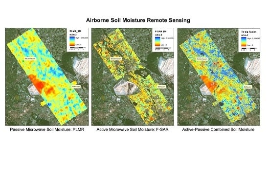
- Pause, M.; Schulz, K.; Zacharias, S.; Lausch, A. Near-surface soil moisture estimation by combining airborne L-band brightness temperature observations and imaging hyperspectral data at the field scale. J. Appl. Remote Sens. 2012, 6, 063516. [Google Scholar]
- Montzka, C.; Grant, J.P.; Moradkhani, H.; Franssen, H.-J.H.; Weihermüller, L.; Drusch, M.; Vereecken, H. Estimation of Radiative Transfer Parameters from L-Band Passive Microwave Brightness Temperatures Using Advanced Data Assimilation. Vadose Zone J. 2013, 12. [Google Scholar] [CrossRef]
- Reigber, A.; Scheiber, R.; Jager, M.; Prats-Iraola, P.; Hajnsek, I.; Jagdhuber, T.; Papathanassiou, K.P.; Nannini, M.; Aguilera, E.; Baumgartner, S.; et al. Very-high-resolution airborne synthetic aperture radar imaging: Signal processing and applications. Proc. IEEE 2013, 101, 759–783. [Google Scholar] [CrossRef]
- Horn, R.; Jaeger, M.; Keller, M.; Limbach, M.; Nottensteiner, A.; Reigber, A.; Scheiber, R. F-SAR—Recent Upgrades and Campaign Activities. In Proceedings of the 18th International Radar Symposium IRS 2017, Prague, Czech Republic, 28–30 June 2017; pp. 2–11. [Google Scholar]
- Montzka, C.; Jagdhuber, T.; Horn, R.; Bogena, H.R.; Hajnsek, I.; Reigber, A.; Vereecken, H. Investigation of SMAP fusion algorithms with airborne active and passive L-Band microwave remote sensing. IEEE Trans. Geosci. Remote Sens. 2016, 54, 3878–3889. [Google Scholar] [CrossRef]
- Panciera, R.; Walker, J.P.; Jackson, T.J.; Gray, D.A.; Tanase, M.A.; Ryu, D.; Monerris, A.; Yardley, H.; Rüdiger, C.; Wu, X.; et al. (SMAPEx): Toward Soil Moisture Retrieval from the SMAP Mission. IEEE Trans. Geosci. Remote Sens. 2014, 52, 490–507. [Google Scholar] [CrossRef]
- Bindlish, R.; Jackson, T.; Sun, R.; Cosh, M.; Yueh, S.; Dinardo, S. Combined passive and active microwave observations of soil moisture during CLASIC. IEEE Geosci. Remote Sens. Lett. 2009, 6, 644–648. [Google Scholar] [CrossRef]
- Konings, A.G.; Entekhabi, D.; Moghaddam, M.; Saatchi, S.S. The Effect of a Variable Soil Moisture Profile on P-band Backscatter Estimation. IEEE Trans. Geosci. Remote Sens. 2014, 52, 6315–6325. [Google Scholar] [CrossRef]
- Kumar, S.V.; Peters-Lidard, C.D.; Mocko, D.; Reichle, R.; Liu, Y.; Arsenault, K.R.; Xia, Y.; Ek, M.; Riggs, G.; Livneh, B.; et al. Assimilation of Remotely Sensed Soil Moisture and Snow Depth Retrievals for Drought Estimation. J. Hydrometeorol. 2014, 15, 2446–2469. [Google Scholar] [CrossRef]
- Montzka, C.; Moradkhani, H.; Weihermüller, L.; Franssen, H.J.H.; Canty, M.; Vereecken, H. Hydraulic parameter estimation by remotely-sensed top soil moisture observations with the particle filter. J. Hydrol. 2011, 399, 410–421. [Google Scholar] [CrossRef]
- Dumedah, G.; Walker, J.P. Intercomparison of the JULES and CABLE land surface models through assimilation of remotely sensed soil moisture in southeast Australia. Adv. Water Resour. 2014, 74, 231–244. [Google Scholar] [CrossRef]
- Ridler, M.-E.; Madsen, H.; Stisen, S.; Bircher, S.; Fensholt, R. Assimilation of SMOS-derived soil moisture in a fully integrated hydrological and soil-vegetation-atmosphere transfermodel in Western Denmark. Water Resour. Res. 2014, 50, 8962–8981. [Google Scholar] [CrossRef]
- Han, X.; Franssen, H.-J.H.; Montzka, C.; Vereecken, H. Soilmoisture and soil properties estimation in the Community Land Model with synthetic brightness temperature observations. Water Resour. Res. 2015, 51, 8757–8772. [Google Scholar]
- Rains, D.; Han, X.; Lievens, H.; Montzka, C.; Verhoest, N.E.C. SMOS brightness temperature assimilation into the Community Land Model. Hydrol. Earth Syst. Sci. Discuss. 2017, 21, 5929–5951. [Google Scholar] [CrossRef]
- Kornelsen, K.C.; Coulibaly, P. Advances in soil moisture retrieval from synthetic aperture radar and hydrological applications. J. Hydrol. 2013, 476, 460–489. [Google Scholar] [CrossRef]
- Wilson, S.M. Use of vegetation-based methods for soil quality assessment in Scottish forestry: A review. Scott. For. 2009, 63, 20–29. [Google Scholar]
- Rudolph, S.; van der Kruk, J.; von Hebel, C.; Ali, M.; Herbst, M.; Montzka, C.; Pätzold, S.; Robinson, D.A.; Vereecken, H.; Weihermüller, L. Linking satellite derived LAI patterns with subsoil heterogeneity using large-scale ground-based electromagnetic induction measurements. Geoderma 2015, 241–242, 262–271. [Google Scholar] [CrossRef]
- Piles, M.; Ballabrera-Poy, J.; Muñoz-Sabater, J. Dominant Features of Global Surface Soil Moisture Variability Observed by the SMOS Satellite. Remote Sens. 2019, 11, 95. [Google Scholar] [CrossRef]
- Huo, A.; Zhang, J.; Cheng, Y.; Yi, X.; Qiao, L.; Su, F.; Du, Y.; Mao, H. Assessing the effect of scaling methods on retrieval of soil moisture based on MODIS images in arid regions. Toxicol. Environ. Chem. 2016, 98, 410–418. [Google Scholar] [CrossRef]
- Li, B.; Ti, C.; Zhao, Y.; Yan, X. Estimating soil moisture with Landsat data and its application in extracting the spatial distribution of winter flooded paddies. Remote Sens. 2016, 8, 38. [Google Scholar] [CrossRef]
- Haubrock, S.-N.; Chabrillat, S.; Kuhnert, M.; Hostert, P.; Kaufmann, H. Surface soil moisture quantification and validation based on hyperspectral data and field measurements. J. Appl. Remote Sens. 2008, 2, 023552. [Google Scholar] [CrossRef]
- Rozenstein, O.; Agam, N.; Serio, C.; Masiello, G.; Venafra, S.; Achal, S.; Puckrin, E.; Karnieli, A. Diurnal emissivity dynamics in bare versus biocrusted sand dunes. Sci. Total Environ. 2015, 506–507, 422–429. [Google Scholar] [CrossRef]
- Martini, E.; Wollschläger, U.; Kögler, S.; Behrens, T.; Dietrich, P.; Reinstorf, F.; Schmidt, K.; Weiler, M.; Werban, U. Spatial and Temporal Dynamics of Hillslope-Scale Soil Moisture Patterns: Characteristic States and Transition Mechanisms. Vadose Zone J. 2013, 14. [Google Scholar] [CrossRef]
- Mitrofanov, I. Maps of Subsurface Hydrogen from the High Energy Neutron Detector, Mars Odyssey. Science 2002, 297, 78–81. [Google Scholar] [CrossRef] [PubMed]
- Baldoncini, M.; Albéri, M.; Bottardi, C.; Chiarelli, E.; Raptis, K.G.C.; Strati, V.; Mantovani, F. Investigating the potentialities of Monte Carlo simulation for assessing soil water content via proximal gamma-ray spectroscopy. J. Environ. Radioact. 2018, 192, 105–116. [Google Scholar] [CrossRef] [PubMed]
- Dierke, C.; Werban, U. Relationships between gamma-ray data and soil properties at an agricultural test site. Geoderma 2013, 199, 90–98. [Google Scholar] [CrossRef]
- Siemon, B.; Costabel, S.; Voß, W.; Meyer, U.; Deus, N.; Elbracht, J.; Günther, T.; Wiederhold, H. Airborne and ground geophysical mapping of coastal clays in Eastern Friesland, Germany. Geophysics 2015, 80, WB21–WB34. [Google Scholar] [CrossRef]
- Priori, S.; Bianconi, N.; Fantappiè, M.; Pellegrini, S.; Ferrigno, G.; Guaitoli, F.; Costantini, E.A. EQA—Environmental quality/Qualité de l’Environnement/Qualità ambientale, 11 (2013) 29–38. EQA Int. J. Environ. Qual. 2013, 11, 29–38. [Google Scholar]
- Guastaldi, E.; Baldoncini, M.; Bezzon, G.; Broggini, C.; Buso, G.; Caciolli, A.; Carmignani, L.; Callegari, I.; Colonna, T.; Dule, K.; et al. A multivariate spatial interpolation of airborne γ-ray data using the geological constraints. Remote Sens. Environ. 2013, 137, 1–11. [Google Scholar] [CrossRef]
- Carroll, T.R. Airborne soil moisture measurement using natural terrestrial gamma radiation. Soil Sci. 1981, 132, 358–366. [Google Scholar] [CrossRef]
- Warren, K.J.; Carroll, T.R. Error analysis of airborne gamma radiation soil moisture measurements. Agric. Meteorol. 1983, 28, 19–30. [Google Scholar]
- Köhli, M.; Schrön, M.; Zreda, M.; Schmidt, U.; Dietrich, P.; Zacharias, S. Footprint characteristics revised for field-scale soil moisture monitoring with cosmic-ray neutrons. Water Resour. Res. 2015, 51, 5772–5790. [Google Scholar] [CrossRef]
- Desilets, D.; Zreda, M.; Ferré, T.P.A. Nature’s neutron probe: Land surface hydrology at an elusive scale with cosmic rays. Water Resour. Res. 2010, 46, W11505. [Google Scholar] [CrossRef]
- Baatz, R.; Bogena, H.R.; Hendricks Franssen, H.-J.; Huisman, J.A.; Montzka, C.; Vereecken, H. An empirical vegetation correction for soil water content quantification using cosmic ray probes. Water Resour. Res. 2015, 51, 2030–2046. [Google Scholar] [CrossRef]
- Schattan, P.; Baroni, G.; Oswald, S.E.; Schöber, J.; Fey, C.; Kormann, C.; Huttenlau, M.; Achleitner, S. Continuous monitoring of snowpack dynamics in alpine terrain by aboveground neutron sensing. Water Resour. Res. 2017, 53, 3615–3634. [Google Scholar] [CrossRef]
- Schrön, M.; Zacharias, S.; Womack, G.; Köhli, M.; Desilets, D.; Oswald, S.E.; Bumberger, J.; Mollenhauer, H.; Kögler, S.; Remmler, P.; et al. Intercomparison of cosmic-ray neutron sensors and water balance monitoring in an urban environment. Geosci. Instrum. Methods Data Syst. 2018, 7, 83–99. [Google Scholar] [CrossRef]
- Franz, T.E.; Wang, T.; Avery, W.; Finkenbiner, C.; Brocca, L. Combined analysis of soil moisture measurements from roving and fixed cosmic ray neutron probes for multiscale real-time monitoring. Geophys. Res. Lett. 2015, 42, 3389–3396. [Google Scholar] [CrossRef]
- Schrön, M.; Rosolem, R.; Köhli, M.; Piussi, L.; Schröter, I.; Iwema, J.; Kögler, S.; Oswald, S.E.; Wollschläger, U.; Samaniego, L.; et al. Cosmic-ray Neutron Rover Surveys of Field Soil Moisture and the Influence of Roads. Water Resour. Res. 2018, 54, 6441–6459. [Google Scholar] [CrossRef]
- Schrön, M. Cosmic-Ray Neutron Sensing and Its Applications to Soil and Land Surface Hydrology. Ph.D. Thesis, University of Potsdam, Potsdam, Germany, 2017. Available online: https://nbn-resolving.org/urn:nbn:de:kobv:517-opus4-395433 (accessed on 02 October 2019).
- Chrisman, B.; Zreda, M. Quantifying mesoscale soil moisture with the cosmic-ray rover. Hydrol. Earth Syst. Sci. 2013, 17, 5097–5108. [Google Scholar] [CrossRef]
- Montzka, C.; Bogena, H.R.; Zreda, M.; Monerris, A.; Morrison, R.; Muddu, S.; Vereecken, H. Validation of Spaceborne and Modelled Surface Soil Moisture Products with Cosmic-Ray Neutron Probes. Remote Sens. 2017, 9, 103. [Google Scholar] [CrossRef]
- Chakrabarti, S.; Bongiovanni, T.; Judge, J.; Zotarelli, L.; Bayer, C. Assimilation of SMOS soil moisture for quantifying drought impacts on crop yield in agricultural regions. IEEE J. Sel. Top. Appl. Earth Obs. Remote Sens. 2014, 7, 3867–3879. [Google Scholar] [CrossRef]
- Merlin, O.; Walker, J.P.; Kalma, J.D.; Kim, E.J.; Hacker, J.; Panciera, R.; Young, R.; Summerell, G.; Hornbuckle, J.; Hafeez, M.; et al. The NAFE’06 data set: Towards soil moisture retrieval at intermediate resolution. Adv. Water Resour. 2008, 31, 1444–1455. [Google Scholar] [CrossRef]
- Kankaku, Y.; Osawa, Y.; Suzuki, S.; Watanabe, T. The Overview of the L-band SAR Onboard ALOS-2. PIERS Proc. Moscow Russ. 2009, 2, 18–21. [Google Scholar]
- Imaoka, K.; Maeda, T.; Kachi, M.; Kasahara, M.; Ito, N.; Nakagawa, K. “Status of AMSR2 Instrument on GCOM-W1”. Proc. SPIE 2012, 8528. [Google Scholar] [CrossRef]
- Gaiser, P.W.; St Germain, K.M.; Twarog, E.M.; Poe, G.A.; Purdy, W.; Richardson, D.; Grossman, W.; Jones, W.L.; Spencer, D.; Golba, G.; et al. The windSat spaceborne polarimetric microwave radiometer: Sensor description and early orbit performance. IEEE Trans. Geosci. Remote Sens. 2004, 42, 2347–2361. [Google Scholar] [CrossRef]
- Bartalis, Z.; Wagner, W.; Naeimi, V.; Hasenauer, S.; Scipal, K.; Bonekamp, H.; Figa, J.; Anderson, C. Initial soil moisture retrievals from the METOP-A Advanced Scatterometer (ASCAT). Geophys. Res. Lett. 2007, 34, 5–9. [Google Scholar] [CrossRef]
- Morena, L.C.; James, K.V.; Beck, J. Technical Note/Note technique An introduction to the RADARSAT-2 mission. Can. J. Remote Sens. 2004, 30, 221–234. [Google Scholar] [CrossRef]
- Misra, T.; Rana, S.S.; Desai, N.M.; Dave, Rajeevjyoti, D.B.; Arora, R.K.; Rao, C.V.N.; Bakori, B.V.; Neelakantan, R.; Vachchani, J.G. Synthetic Aperture Radar payload on-board RISAT-1: Configuration, technology and performance. Curr. Sci. 2013, 104, 446–461. [Google Scholar]
- Torres, R.; Snoeij, P.; Geudtner, D.; Bibby, D.; Davidson, M.; Attema, E.; Potin, P.; Rommen, B.; Floury, N.; Brown, M.; et al. GMES Sentinel-1 mission. Remote Sens. Environ. 2012, 120, 9–24. [Google Scholar] [CrossRef]
- Krieger, G.; Moreira, A.; Fiedler, H.; Hajnsek, I.; Werner, M.; Younis, M.; Zink, M. TanDEM-X: A satellite formation for high-resolution SAR interferometry. IEEE Trans. Geosci. Remote Sens. 2007, 45, 3317–3340. [Google Scholar] [CrossRef]
- Werninghaus, R.; Buckreuss, S. The TerraSAR-X mission and system design. IEEE Trans. Geosci. Remote Sens. 2010, 48, 606–614. [Google Scholar] [CrossRef]
- Pasolli, L.; Notarnicola, C.; Bertoldi, G.; Della Chiesa, S.; Niedrist, G.; Bruzzone, L.; Tappeiner, U.; Zebisch, M. Soil moisture monitoring in mountain areas by using high-resolution SAR images: Results from a feasibility study. Eur. J. Soil Sci. 2014, 65, 852–864. [Google Scholar] [CrossRef]
- Panciera, R.; Walker, J.P.; Kalma, J.D.; Kim, E.J.; Member, S.; Hacker, J.M.; Merlin, O.; Berger, M.; Skou, N.; The, A.; et al. The NAFE’ 05/CoSMOS Data Set: Toward SMOS Soil Moisture Retrieval, Downscaling, and Assimilation. Cosmos 2008, 46, 1–10. [Google Scholar] [CrossRef]
- Jiang, T.; Zhao, K.; Zheng, X.; Chen, S.; Wan, X. Dynamic bp in the L Band and Its Role in Improving the Accuracy of Soil Moisture Retrieval. Chin. Geogr. Sci. 2019, 29, 283–292. [Google Scholar] [CrossRef]
- Panciera, R.; Walker, J.P.; Kim, E.; Kalma, J.; Merlin, O.; Oxley, L.; Kulasiri, D. Effect of Spatial Scale on Soil Moisture Retrieval from Passive Microwave Sensors. In Proceedings of the Modsim 2007 International Congress on Modelling and Simulation, Christchurch, New Zealand, 10–13 December 2007; pp. 2576–2582. [Google Scholar]
- Narayan, U.; Lakshmi, V.; Njoku, E.G. Retrieval of soil moisture from passive and active L/S band sensor (PALS) observations during the Soil Moisture Experiment in 2002 (SMEX02). Remote Sens. Environ. 2004, 92, 483–496. [Google Scholar] [CrossRef]
- Kim, J.; Hogue, T.S. Improving spatial soil moisture representation through integration of AMSR-E and MODIS products. IEEE Trans. Geosci. Remote Sens. 2012, 50, 446–460. [Google Scholar] [CrossRef]
- Jarmer, T.; Lavée, H.; Sarah, P.; Hill, J. Using reflectance spectroscopy and landsat data to assess soil inorganic carbon in the Judean Desert (Israel). In Recent Advances in Remote Sensing and Geoinformation Processing for Land Degradation Assessment; Röder, A., Hill, J., Eds.; CRC Press: London, UK, 2009; pp. 227–243. ISBN 9780203875445. [Google Scholar]
- Zhang, Z.; He, G.; Wang, M.; Long, T.; Wang, G.; Zhang, X.; Jiao, W. Towards an operational method for land surface temperature retrieval from Landsat 8 data. Remote Sens. Lett. 2016, 7, 279–288. [Google Scholar] [CrossRef]
- Sobrino, J.A.; Franch, B.; Mattar, C.; Jiménez-muñoz, J.C.; Corbari, C. A method to estimate soil moisture from Airborne Hyperspectral Scanner (AHS) and ASTER data: Application to SEN2FLEX and SEN3EXP campaigns. Remote Sens. Environ. 2012, 117, 415–428. [Google Scholar] [CrossRef]
- Gao, Q.; Zribi, M.; Escorihuela, M.J. Synergetic Use of Sentinel-1 and Sentinel-2 Data for Soil Moisture Mapping at 100 m Resolution. Sensors 2017, 17, 1966. [Google Scholar] [CrossRef] [PubMed]
- Fabre, S.; Briottet, X.; Lesaignoux, A.; Avenue, B.P.; Belin, E.; Cedex, F.-T. Estimation of Soil Moisture Content from the Spectral Reflectance of Bare Soils in the 0.4–2.5 μm Domain. Sensors 2015, 15, 3262–3281. [Google Scholar] [CrossRef] [PubMed]
- Klinke, R.; Kuechly, H.; Frick, A.; Förster, M.; Schmidt, T.; Holtgrave, A.K.; Kleinschmit, B.; Spengler, D.; Neumann, C. Indicator-Based Soil Moisture Monitoring of Wetlands by Utilizing Sentinel and Landsat Remote Sensing Data. PFG J. Photogramm. Remote Sens. Geoinf. Sci. 2018, 86, 71–84. [Google Scholar] [CrossRef]
- Dorigo, W.A.; Wagner, W.; Hohensinn, R.; Hahn, S.; Paulik, C.; Xaver, A.; Gruber, A.; Drusch, M.; Mecklenburg, S.; Van Oevelen, P.; et al. The International Soil Moisture Network: A data hosting facility for global in situ soil moisture measurements. Hydrol. Earth Syst. Sci. 2011, 15, 1675–1698. [Google Scholar] [CrossRef]
- Das, N.N.; Entekhabi, D.; Dunbar, R.S.; Chaubell, M.J.; Colliander, A.; Yueh, S.; Jagdhuber, T.; Chen, F.; Crow, W.; O’Neill, P.E.; et al. The SMAP and Copernicus Sentinel 1A/B microwave active-passive high resolution surface soil moisture product. Remote Sens. Environ. 2019, 233, 111380. [Google Scholar] [CrossRef]
- Colliander, A.; Jackson, T.J.; Chan, S.K.; Neill, P.O.; Bindlish, R.; Cosh, M.H.; Caldwell, T.; Walker, J.P.; Berg, A.; Mcnairn, H.; et al. An assessment of the di ff erences between spatial resolution and grid size for the SMAP enhanced soil moisture product over homogeneous sites. Remote Sens. Environ. 2018, 207, 65–70. [Google Scholar] [CrossRef]
- Bitar, A.A.; Mialon, A.; Kerr, Y.H.; Cabot, F.; Richaume, P.; Jacquette, E.; Quesney, A.; Mahmoodi, A.; Tarot, S.; Parrens, M.; et al. The global SMOS Level 3 daily soil moisture and brightness temperature maps. Earth Syst. Sci. Data 2017, 9, 293–315. [Google Scholar] [CrossRef]
- Rodell, M.; Houser, P.R.; Jambor, U.; Gottschalck, J.; Mitchell, K.; Meng, C.-J.; Arsenault, K.; Cosgrove, B.; Radakovich, J.; Bosilovich, M.; et al. The Global Land Data Assimilation System. Bull. Am. Meteorol. Soc. 2004, 85, 381–394. [Google Scholar] [CrossRef]
- Houborg, R.; Rodell, M.; Li, B.; Reichle, R.; Zaitchik, B.F. Drought indicators based on model-assimilated Gravity Recovery and Climate Experiment (GRACE) terrestrial water storage observations. Water Resour. Res. 2012, 48. [Google Scholar] [CrossRef]
- Kustas, W.P.; French, A.N.; Hatfield, J.L.; Jackson, T.J.; Susan Moran, M.; Rango, A.; Ritchie, J.C.; Schmugge, T.J.; Moran, M.S.; Rango, A.; et al. Remote Sensing Research in Hydrometeorology. Photogramm. Eng. Remote Sens. 2003, 69, 631–646. [Google Scholar] [CrossRef]
- Karnieli, A.; Agam, N.; Pinker, R.T.; Anderson, M.; Imhoff, M.L.; Gutman, G.G.; Panov, N.; Goldberg, A. Use of NDVI and land surface temperature for drought assessment: Merits and limitations. J. Clim. 2010, 23, 618–633. [Google Scholar] [CrossRef]
- Zink, M. Conditioning a Hydrologic Model Using Patterns of Remotely Sensed Land Surface Temperature. Water Resour. Res. 2018, 54, 2976–2998. [Google Scholar] [CrossRef]
- Li, Z.-L.; Tang, B.-H.; Wu, H.; Ren, H.; Yan, G.; Wan, Z.; Trigo, I.F.; Sobrino, J.A. Satellite-derived land surface temperature: Current status and perspectives. Remote Sens. Environ. 2013, 131, 14–37. [Google Scholar] [CrossRef]
- Costa, J.M.; Grant, O.M.; Chaves, M.M. Thermography to explore plant—Environment interactions. J. Exp. Bot. 2013, 64, 3937–3949. [Google Scholar] [CrossRef]
- Townshend, J.R.; Justice, C.O.; Skole, D.; Malingreau, J.P.; Cihlar, J.; Teillet, P.; Sadowski, F.; Ruttenberg, S. The 1 km resolution global data set: Needs of the international geosphere biosphere programme! Int. J. Remote Sens. 1994, 15, 3417–3441. [Google Scholar] [CrossRef]
- Weber, N.; Haase, D.; Franck, U. Science of the Total Environment Zooming into temperature conditions in the city of Leipzig: How do urban built and green structures in fl uence earth surface temperatures in the city? Sci. Total Environ. 2014, 496, 289–298. [Google Scholar] [CrossRef] [PubMed]
- Kalma, J.D.; McVicar, T.R.; McCabe, M.F. Estimating land surface evaporation: A review of methods using remotely sensed surface temperature data. Surv. Geophys. 2008, 29, 421–469. [Google Scholar] [CrossRef]
- Hansen, J.; Ruedy, R.; Sato, M.; Lo, K. Global surface temperature change. Rev. Geophys. 2010, 48. [Google Scholar] [CrossRef]
- Krajewski, W.F.; Anderson, M.C.; Eichinger, W.E.; Entekhabi, D.; Hornbuckle, B.K.; Houser, P.R.; Katul, G.G.; Kustas, W.P.; Norman, J.M.; Peters-Lidard, C.; et al. A remote sensing observatory for hydrologic sciences: A genesis for scaling to continental hydrology. Water Resour. Res. 2006, 42, 1–13. [Google Scholar] [CrossRef]
- Brenner, C.; Zeeman, M.; Bernhardt, M.; Schulz, K. Estimation of evapotranspiration of temperate grassland based on high-resolution thermal and visible range imagery from unmanned aerial systems. Int. J. Remote Sens. 2018, 39, 5141–5174. [Google Scholar] [CrossRef]
- Brenner, C.; Thiem, C.E.; Wizemann, H.D.; Bernhardt, M.; Schulz, K. Estimating spatially distributed turbulent heat fluxes from high-resolution thermal imagery acquired with a UAV system. Int. J. Remote Sens. 2017, 38, 3003–3026. [Google Scholar] [CrossRef]
- Bonan, G.B. Ecological Climatology: Concepts and Applications, 2nd Edition. Geogr. Res. 2008, 48, 221–222. [Google Scholar]
- Müller, B.; Bernhardt, M.; Schulz, K. Identification of catchment functional units by time series of thermal remote sensing images. Hydrol. Earth Syst. Sci. 2014, 18, 5345–5359. [Google Scholar] [CrossRef]
- Neteler, M. Estimating daily land surface temperatures in mountainous environments by reconstructed MODIS LST data. Remote Sens. 2010, 2, 333–351. [Google Scholar] [CrossRef]
- Li, Z.-L.; Becker, F. Feasibility of land surface temerature and emissivity determination from AVHRR data. Remote Sens. Environ. 1993, 43, 67–85. [Google Scholar] [CrossRef]
- Hoffmann, H.; Nieto, H.; Jensen, R.; Guzinski, R.; Zarco-Tejada, P.; Friborg, T. Estimating evaporation with thermal UAV data and two-source energy balance models. Hydrol. Earth Syst. Sci. 2016, 20, 697–713. [Google Scholar] [CrossRef]
- Malbéteau, Y.; Parkes, S.; Aragon, B.; Rosas, J.; McCabe, M.F. Capturing the diurnal cycle of land surface temperature using an unmanned aerial vehicle. Remote Sens. 2018, 10, 1407. [Google Scholar] [CrossRef]
- Ghent, D.; Veal, K.; Trent, T.; Remedios, J. A New Approach to Defining Uncertainties for MODIS Land Surface Temperature. Remote Sens. 2019, 11, 1021. [Google Scholar] [CrossRef]
- Raoufi, R.; Beighley, E. Estimating daily global evapotranspiration using penman-monteith equation and remotely sensed land surface temperature. Remote Sens. 2017, 9, 1138. [Google Scholar] [CrossRef]
- Coll, C.; Caselles, V.; Galve, J.M.; Valor, E.; Niclòs, R.; Sánchez, J.M.; Rivas, R. Ground measurements for the validation of land surface temperatures derived from AATSR and MODIS data. Remote Sens. Environ. 2005, 97, 288–300. [Google Scholar] [CrossRef]
- Hook, S.J.; Vaughan, R.G.; Tonooka, H.; Schladow, S.G. Absolute Radiometric in-Flight Validation of Mid Infrared and Thermal Infrared Data from ASTER and MODIS on the Terra Spacecraft Automated Validation Site. IEEE Trans. Geosci. Remote Sens. 2007, 45, 1798–1807. [Google Scholar] [CrossRef]
- Cristóbal, J.; Jiménez-Muñoz, J.C.; Sobrino, J.A.; Ninyerola, M.; Pons, X. Improvements in land surface temperature retrieval from the Landsat series thermal band using water vapor and air temperature. J. Geophys. Res. Atmos. 2009, 114, 1–16. [Google Scholar] [CrossRef]
- Jiménez-Muñoz, J.C.; Cristóbal, J.; Sobrino, J.A.; Sòria, G.; Ninyerola, M.; Pons, X. Revision of the single-channel algorithm for land surface temperature retrieval from landsat thermal-infrared data. IEEE Trans. Geosci. Remote Sens. 2009, 47, 339–349. [Google Scholar] [CrossRef]
- Rozenstein, O.; Qin, Z.; Derimian, Y.; Karnieli, A. Derivation of Land Surface Temperature for Landsat-8 TIRS Using a Split Window Algorithm. Sensors 2014, 14, 5768–5780. [Google Scholar] [CrossRef] [PubMed]
- Petitcolin, F.; Nerry, F.; Stoll, M.P. Mapping temperature independent spectral indice of emissivity and directional emissivity in AVHRR channels 4 and 5. Int. J. Remote Sens. 2002, 23, 3473–3491. [Google Scholar] [CrossRef]
- Pinheiro, A.C.T.; Privette, J.L.; Mahoney, R.; Tucker, C.J. Directional effects in a daily AVHRR land surface temperature dataset over Africa. IEEE Trans. Geosci. Remote Sens. 2004, 42, 1941–1954. [Google Scholar] [CrossRef]
- Coll, C.; Caselles, V.; Valor, E.; Niclòs, R.; Sánchez, J.M.; Galve, J.M.; Mira, M. Temperature and emissivity separation from ASTER data for low spectral contrast surfaces. Remote Sens. Environ. 2007, 110, 162–175. [Google Scholar] [CrossRef]
- Guzinski, R.; Nieto, H. Evaluating the feasibility of using Sentinel-2 and Sentinel-3 satellites for high-resolution evapotranspiration estimations. Remote Sens. Environ. 2019, 221, 157–172. [Google Scholar] [CrossRef]
- Qing, S.; Zhang, J.; Cui, T.; Bao, Y. Retrieval of sea surface salinity with MERIS and MODIS data in the Bohai Sea. Remote Sens. Environ. 2013, 136, 117–125. [Google Scholar] [CrossRef]
- Jiang, G.-M.; Li, Z.-L. Split-window algorithm for land surface temperature estimation from MSG1-SEVIRI data. Int. J. Remote Sens. 2008, 29, 6067–6074. [Google Scholar] [CrossRef]
- Huang, M.; Lee, P.; Mcnider, R.; Crawford, J.; Buzay, E.; Barrick, J.; Liu, Y.; Krishnan, P. Temporal and spatial variability of daytime land surface temperature in Houston: Comparing DISCOVER-AQ aircraft observations with the WRF model and satellites. J. Geophys. Res. Atmos. 2016, 121, 185–195. [Google Scholar] [CrossRef]
- Sobrino, J.A.; Jiménez-muñoz, J.C.; Zarco-tejada, P.J.; Sepulcre-cantó, G.; De Miguel, E. Land surface temperature derived from airborne hyperspectral scanner thermal infrared data. Remote Sens. Environ. 2006, 102, 99–115. [Google Scholar] [CrossRef]
- Adler-Golden, S.; Conforti, P.; Gagnon, M.A.; Tremblay, P.; Chamberland, M. Remote sensing of surface emissivity with the telops Hyper-Cam. In Proceedings of the 2014 6th Workshop on Hyperspectral Image and Signal Processing: Evolution in Remote Sensing (WHISPERS), Lausanne, Switzerland, 24–27 June 2014; pp. 9–12. [Google Scholar]
- Gagnon, M.-A.; Tremblay, P.; Savary, S.; Farley, V.; Lagueux, P.; Chamberland, M. Airborne thermal hyperspectral imaging of urban and rural areas. In Proceedings of the 2014 IEEE Geoscience and Remote Sensing Symposium, Quebec, QC, Canada, 13–18 July 2014; IEEE: Piscataway, NJ, USA, 2014; pp. 1369–1372. [Google Scholar]
- Galleguillos, M.; Jacob, F.; Prévot, L.; French, A.; Lagacherie, P. Comparison of two temperature differencing methods to estimate daily evapotranspiration over a Mediterranean vineyard watershed from ASTER data. Remote Sens. Environ. 2011, 115, 1326–1340. [Google Scholar] [CrossRef]
- Anderson, M.C.; Allen, R.G.; Morse, A.; Kustas, W.P. Use of Landsat thermal imagery in monitoring evapotranspiration and managing water resources. Remote Sens. Environ. 2012, 122, 50–65. [Google Scholar] [CrossRef]
- Dold, C.; Heitman, J.; Giese, G.; Howard, A.; Havlin, J.; Sauer, T. Upscaling Evapotranspiration with Parsimonious Models in a North Carolina Vineyard. Agronomy 2019, 9, 152. [Google Scholar] [CrossRef]
- Parastatidis, D.; Mitraka, Z.; Chrysoulakis, N.; Abrams, M. Online Global Land Surface Temperature Estimation from Landsat. Remote Sens. 2017, 9, 1208. [Google Scholar] [CrossRef]
- GLCF; GSFC. Landsat Surface Reflectance, Landsat TM & ETM+; Global Land Cover Facility, University of Maryland: College Park, MD, USA, 2011. [Google Scholar]
- Liang, S.; Zhang, X. Global Land Surface Products: Shortwave Radiation Product Data Collection (2008–2010); Beijing Normal University: Beijing, China, 2012. [Google Scholar] [CrossRef]
- Kissling, W.D.; Walls, R.; Bowser, A.; Jones, M.O.; Kattge, J.; Agosti, D.; Amengual, J.; Basset, A.; van Bodegom, P.M.; Cornelissen, J.H.C.; et al. Towards global data products of Essential Biodiversity Variables (EBVs) on species traits. Nat. Ecol. Evol. 2018, 2, 1531–1540. [Google Scholar] [CrossRef] [PubMed]
- Lausch, A.; Schmidt, A.; Tischendorf, L. Data mining and linked open data—New perspectives for data analysis in environmental research. Ecol. Model. 2015, 295, 5–17. [Google Scholar] [CrossRef]
- Bereta, K.; Koubarakis, M.; Pantazi, D.A.; Stamoulis, G.; Caumont, H.; Daniels, U.; Dirk, D.; Ubels, S.; Venus, V.; Wahyudi, F. Providing Satellite Data to Mobile Developers Using Semantic Technologies and Linked Data. In Proceedings of the ICSC 2019: IEEE International Conference on Semantic Computing, Newport Beach, CA, USA, 30 January–1 February 2019; pp. 348–351. [Google Scholar]
- Haase, P.; Tonkin, J.D.; Stoll, S.; Burkhard, B.; Frenzel, M.; Geijzendorffer, I.R.; Häuser, C.; Klotz, S.; Kühn, I.; McDowell, W.H.; et al. The next generation of site-based long-term ecological monitoring: Linking essential biodiversity variables and ecosystem integrity. Sci. Total Environ. 2018, 613–614, 1376–1384. [Google Scholar] [CrossRef]


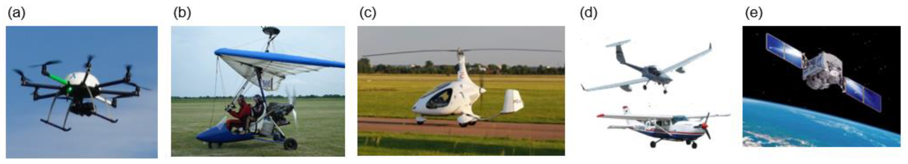
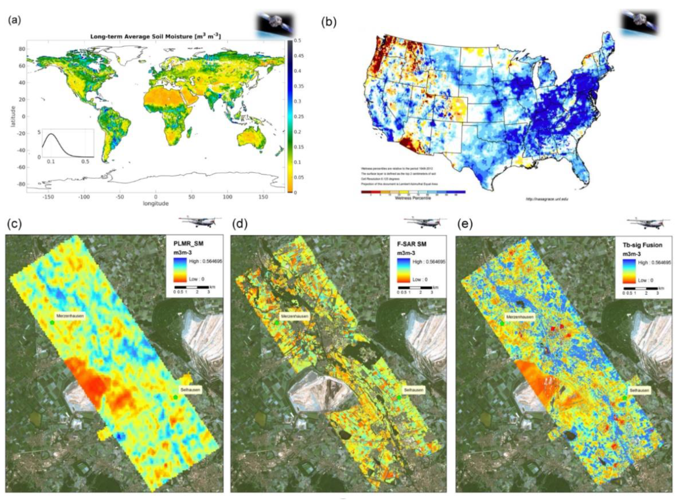
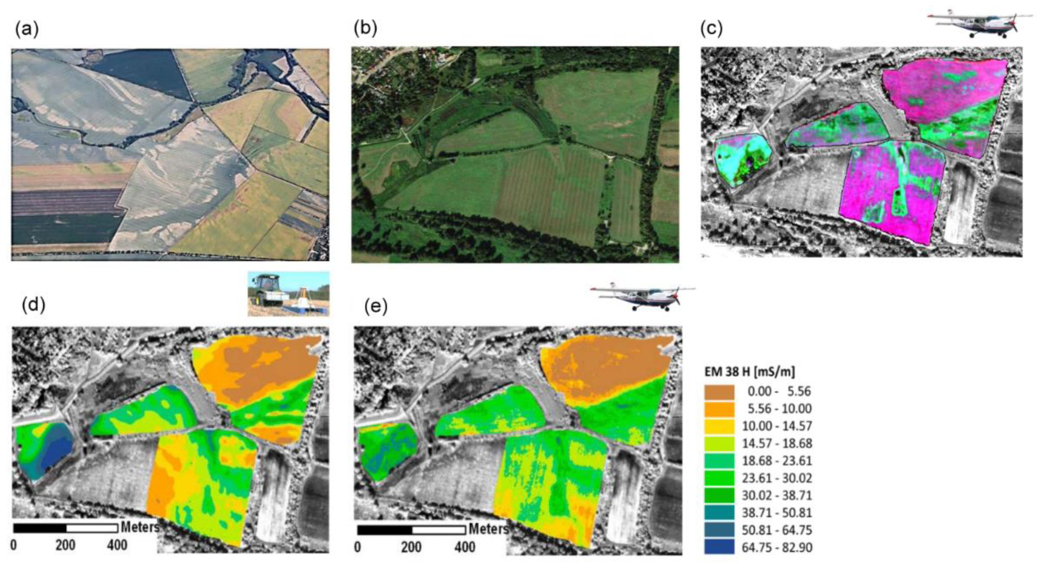
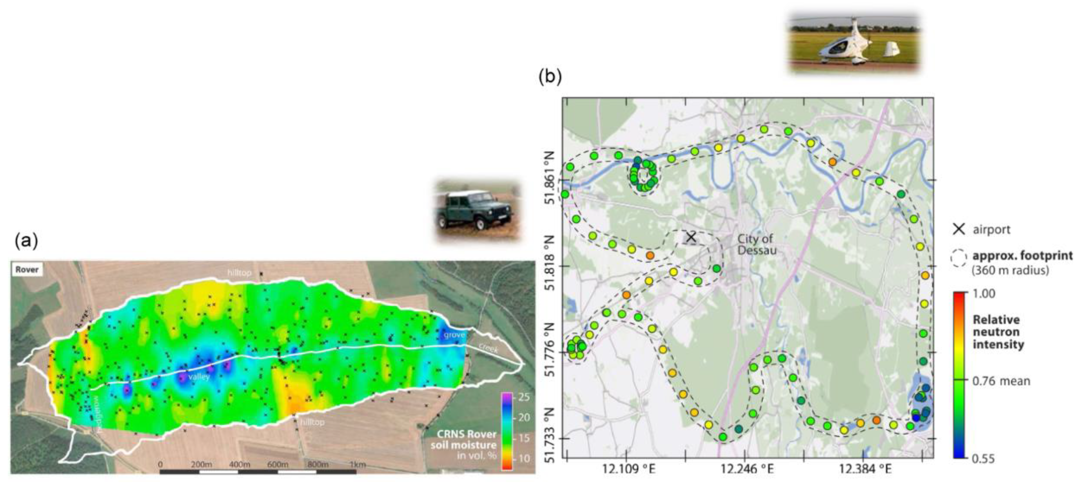
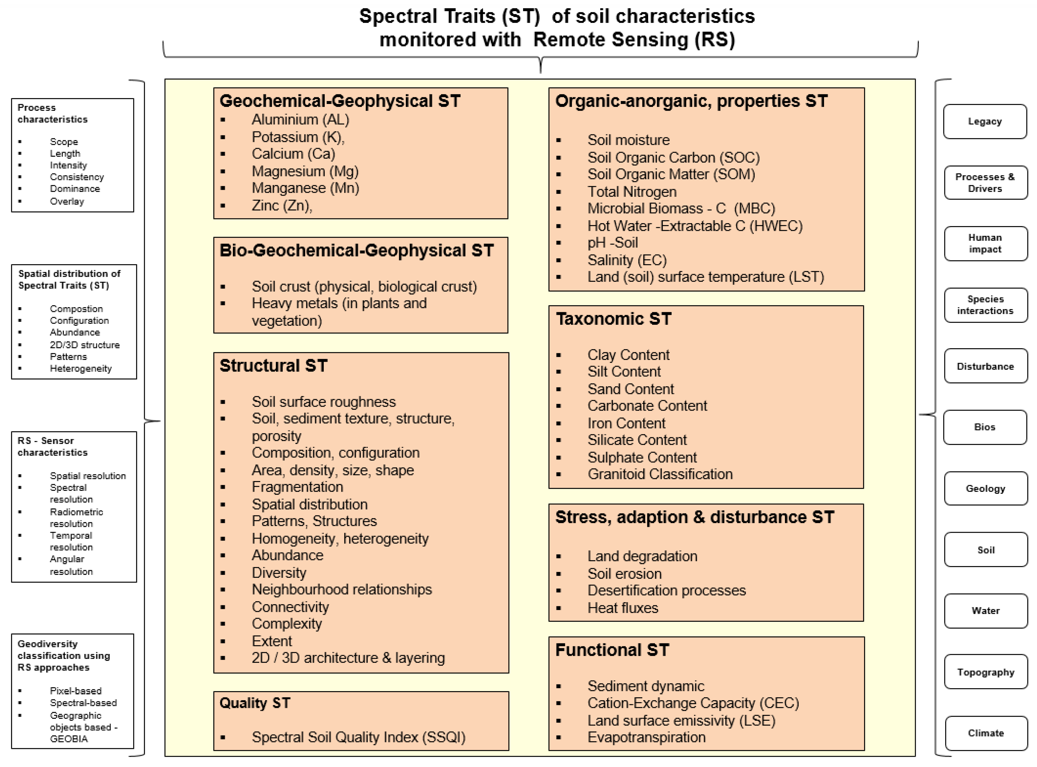
| Mission/Sensor/ Platform UAV 1 Airborne 2 Spaceborne 3 | Sensor Type | Spectral Resolution Spectral Bands/Frequency | Spatial Resolution [m] | References |
|---|---|---|---|---|
| Clay Content | ||||
| Landsat 5 TM 3 Landsat 7 ETM+ 3 | Multispectral/TIR | 0.45–12.5 μm/8 | L5:30/120 L7:30/60 | [68] |
| Landsat 8 OLI/TIRS 3 | Multispectral/TIR | 0.43–2.3 μm/8 10.6–12.51 μm/2 | 30/100 | [68] |
| Terra ASTER 3 | Multispectral/TIR | 0.52–9.2 μm/9 8.12–11.65 μm/5 | 30/90 | [68,80,85] |
| Sentinel–2 MSI 3 | Multispectral | 0.40 3.0 μm/13 | 10/20/60 | [68] |
| IKONOS OSA3 | Multispectral | 0.45–0.85 μm/4 | 4 | [152] |
| AHS 2 | Hyperspectral | 0.43–12.7 μm/~80 | ~2 | [88] |
| AisaDUAL 2 | Hyperspectral | 0.40–2.45 μm/~200–400 | ~1–5 | [68,151] |
| AisaOWL 2 | Hyperspectral Longwave Infrared (LWIR) | 7.7–12.0 μm/~100 | ~2 | [89,90] |
| AVNIR 2 | Hyperspectral | 0.43–1.01 μm/~60 | ~1.20 | [153] |
| AVIRIS 2 | Hyperspectral | 0.37–2.45 μm/~200 | ~18 | [67,154] |
| DAIS-7915 2 | Hyperspectral | 0.40–2.50 μm/~72 | ~8 | [130] |
| EnMAP 2 (simulated) | Hyperspectral | 0.42–2.45 μm/~250 | 30 | [155] |
| HyMAP 2 | Hyperspectral | 0.45–2.48 μm/~125 | ~5 | [84,115,116,117,123,131,156] |
| HySpex 2 | Hyperspectral | 0.40–2.45 μm /~200–400 | ~1–5 | [157] |
| HyperSpecTIR 2 | Hyperspectral | 0.40–2.45 μm/~178 | ~2.5 | [158] |
| TASI-600 2 | Thermal Airborne Spectrographic Imager | 8.0–11.4 μm/~32 | ~1–5 | [84,85] |
| SEBASS 2 | Hyperspectral Thermal Infrared (TIR) Sensor | 2.5–13.5 μm/~260 | ~2 | [87,95] |
| Cubert UHD 185 1 | Hyperspectral | 0.45–0.95 μm/~125 | ~ 0.2–0.5 | [95] |
| Silt Content | ||||
| AisaDUAL 2 | Hyperspectral | 0.40–2.45 μm /~200–400 | ~1–5 | [133] |
| HyperSpecTIR 2 | Hyperspectral | 0.40–2.45 μm/~178 | ~2.5 | [158] |
| Sand Content | ||||
| EO-1 Hyperion 3 | Hyperspectral | 0.40–2.50/242 μm/220 | 30 | [159] |
| AisaDUAL 2 | Hyperspectral | 0.40–2.45 μm /~200–400 | ~1–5 | [133] |
| HyMAP 2 | Hyperspectral | 0.45–2.48 μm/~125 | ~5 | [84] |
| HyperSpecTIR 2 | Hyperspectral | 0.40–2.45 μm/~178 | ~2.5 | [158] |
| TASI-600 2 | Thermal Airborne Spectrographic Imager | 8.0–11.4 μm/~32 | ~1–5 | [84] |
| Carbonate Content | ||||
| Terra ASTER 3 | Multispectral/TIR | 0.52–9.2 μm/9 8.12–11.65 μm/5 | 30/90 | [76,79,80,85] |
| AVIRIS 2 | Hyperspectral | 0.37–2.45 μm/~200 | ~18 | [67] |
| HySpex 2 | Hyperspectral | 0.40–2.45 μm/~200–400 | ~1–5 | [115,116] |
| HyMAP 2 | Hyperspectral | 0.45–2.48 μm/~125 | ~5 | [117,156,160] |
| HyperSpecTIR 2 | Hyperspectral | 0.40–2.45 μm/~178 | ~2.5 | [158] |
| AisaOWL 2 | Hyperspectral Longwave Infrared (LWIR) | 7.7–12.0 μm/~100 | ~2 | [89] |
| SEBASS 2 | Hyperspectral Thermal Infrared (TIR) Sensor | 2.5–13.5 μm/~260 | ~2 | [86,87,95] |
| Iron Content | ||||
| Terra ASTER 3 | Multispectral/TIR | 0.52–9.2 μm/9 8.12–11.65 μm/5 | 30/90 | [76] |
| Sentinel-2 MSI 3 | Multispectral | 0.40 3.0 μm/13 | 10/20/60 | [76] |
| EnMAP 2 (simulated) | Hyperspectral | 0.42–2.45 μm/~250 | 30 | [155] |
| CASI 2 | Hyperspectral | 0.40–1.0/ 48 | ~3 | [137] |
| HyMAP 2 | Hyperspectral | 0.45–2.48 μm/~125 | ~5 | [98,117,155] |
| HySpex 2 | Hyperspectral | 0.40–2.45 μm /~200–400 | ~1–5 | [98,155] |
| HyperSpecTIR 2 | Hyperspectral | 0.40–2.45 μm/~178 | ~2.5 | [158] |
| ROSIS 2 | Hyperspectral | 0.42–0.87/ 115 | ~2 | [161] |
| TASI-600 2 | Thermal Airborne Spectrographic Imager | 8.0–11.4 μm/~32 | ~1–5 | [84] |
| Heavy metals (in plants and vegetation) | ||||
| HyMAP 2 | Hyperspectral | 0.45–2.48 μm/~125 | ~5 | [162] |
| Silicate Content | ||||
| Terra ASTER 3 | Multispectral/TIR | 0.52–9.2 μm/9 8.12–11.65 μm/5 | 30/90 | [76,80] |
| AHS 2 | Hyperspectral | 0.43–12.7 μm/~80 | ~2 | [88] |
| AisaOWL 2 | Hyperspectral Longwave Infrared (LWIR) | 7.7–12.0 μm/~100 | ~2 | [89,91] |
| HyMAP 2 | Hyperspectral | 0.45–2.48 μm/~125 | ~5 | [84] |
| SEBASS 2 | Hyperspectral Thermal Infrared (TIR) Sensor | 2.5–13.5 μm/~260 | ~2 | [86,87,95] |
| TASI-600 2 | Thermal Airborne Spectrographic Imager | 8.0–11.4 μm/~32 | ~1–5 | [85] |
| Sulphate Content | ||||
| Terra ASTER 3 | Multispectral/TIR | 0.52–9.2 μm/9 8.12–11.65 μm/5 | 30/90 | [80] |
| AisaOWL 2 | Hyperspectral Longwave Infrared (LWIR) | 7.7–12.0 μm/~100 | ~2 | [89] |
| AisaFENIX 2 | Hyperspectral | 0.40–2.45 μm/~200–400 | ~1–5 | [90] |
| AVIRIS 2 | Hyperspectral | 0.37–2.45 μm/~200 | ~18 | [67] |
| SEBASS 2 | Hyperspectral Thermal Infrared (TIR) Sensor | 2.5–13.5 μm/~260 | ~2 | [87,95] |
| Granitoid Classification | ||||
| TASI-600 2 | Thermal Airborne Spectrographic Imager | 8.0–11.4 μm/~32 | ~1–5 | [92] |
| Further Elements: (Chemometric diversity of soil) Aluminium (AL), Potassium (K), Calcium (Ca), Magnesium (Mg), Manganese (Mn), Zinc (Zn), (Nt) | ||||
| HyperSpecTIR 2 | Hyperspectral | 0.40–2.450 μm/~178 | 2.5 | [158] |
| HyMAP 2 | Hyperspectral | 0.45–2.48 μm/~125 | ~5 | [131,132] |
| Soil Organic Carbon (SOC) | ||||
| Terra ASTER 3 | Multispectral/TIR | 0.52–9.2 μm/9 8.12–11.65 μm/5 | 30/90 | [163] |
| Sentinel-2 MSI 3 | Multispectral | 0.40 –3.0 μm/13 | 10/20/60 | [164] |
| EO-1 Hyperion 3 | Hyperspectral | 0.40–2.50/242 μm/196 | 30 | [115] |
| AHS 2 | Hyperspectral | 0.43–12.7 μm/~80 | ~2 | [118] |
| AisaDUAL 2 | Hyperspectral | 0.40–2.45 μm/~200–400 | ~1–5 | [133] |
| APEX 2 | Hyperspectral | 0.40–2.50 μm/~320 | ~1–3 | [113] |
| AVNIR 2 | Hyperspectral | 0.43–1.01 μm/~60 | ~1.20 | [153] |
| DAIS-7915 2 | Hyperspectral | 0.40–2.50 μm/72 | 8 | [130] |
| EnMAP 2 (simulated) | Hyperspectral | 0.42–2.45 μm/~250 | 30 | [155] |
| HyMAP 2 | Hyperspectral | 0.45–2.48 μm/~125 | ~5 | [84,123,127,131,132,165] |
| TASI-600 2 | Thermal Airborne Spectrographic Imager | 8.0–11.4 μm/~32 | ~1–5 | [84] |
| Soil Organic Matter (SOM) | ||||
| HyMAP 2 | Hyperspectral | 0.45–2.48 μm/~125 | ~5 | [84] |
| TASI–600 2 | Thermal Airborne Spectrographic Imager | 8.0–11.4 μm/~32 | ~1–5 | [84]. |
| HyperSpecTIR 2 | Hyperspectral | 0.40–2.45 μm/~178 | ~2.5 | [158] |
| Total Nitrogen | ||||
| HyMAP 2 | Hyperspectral | 0.45–2.48 μm/~125 | ~5 | [131,132] |
| Microbial Biomass C (MBC) | ||||
| HyMAP 2 | Hyperspectral | 0.45–2.48 μm/~125 | ~5 | [132] |
| Hot Water Extractable C (HWEC) | ||||
| HyMAP 2 | Hyperspectral | 0.45–2.48 μm/~125 | ~5 | [132] |
| pH -Soil | ||||
| HyperSpecTIR 2 | Hyperspectral | 0.40–2.45 μm/~178 | ~2.5 | [158] |
| Salinity (EC) | ||||
| Landsat 5 TM 3 Landsat 7 ETM+ 3 | Multispectral/TIR | 0.45–2.3 μm/6 10.4–12.5 μm/1 | L5:30/120 L7:30/60 | [166,167] |
| Landsat 8 OLI/TIRS 3 | Multispectral/TIR | 0.43–2.3 μm/8 10.6–12.51 μm/2 | 30/100 | [168] |
| Sentinel-2 MSI 3 | Multispectral | 0.40 –3.0 μm/13 | 10/20/60 | [169] |
| HyMAP 2 | Hyperspectral | 0.45–2.48 μm/~125 | ~5 | [130,170] |
| AIRSAR TOPSAR 2 | Microwave | P–, L-bands (full polarimetric), C-band (VV polarization) | [171] | |
| JERS-1 3 | Microwave | L-band (23 cm)-HH pol | [171] | |
| Cation-Exchange Capacity (CEC) | ||||
| HyMAP 2 | Hyperspectral | 0.45–2.48 μm/~125 | ~5 | [117,139] |
| Soil crust (physical, biological crust) | ||||
| Landsat 5 TM 3 Landsat 7 ETM+ 3 | Multispectral/TIR | 0.45–2.3 μm/6 10.4–12.5 μm/1 | L5:30/120 L7:30/60 | [172] |
| AISA-EAGLE 2 | Hyperspectral | 0.42–0.89 μm/~30 | ~3 | [173] |
| DAIS-791 2 | Hyperspectral | 0.50–2.50 μm/~72 | ~1–3 | [174] |
| CASI 2 | Hyperspectral | 0.42–0.95 μm/~36 | ~1 | [175] |
| Soil surface roughness | ||||
| TerraSAR-X/TanDEM-X 3 | X-band | 9.63 GHz | [176] | |
| Sentinel-1 3 | C-band | 5.3 GHz | [177] | |
| PLMR 2 InfraTec thermal imager 2 AISA-EAGLE 2 | L-band microwave radiometer / TIR/ Hyperspectral | 1.26 GHz 7.5–14 μm 0.42–0.89 μm/~30 | ~3–5 | [178] |
| Riegl-LMS-Q560 full-waveform 2D laser scanner-LiDAR 2 | LiDAR | 240 KHz | [179] | |
| RGB-Camera-UAV 1 | Photogrammetry | ~1–4mm | [180] | |
| Soil texture, sediment texture | ||||
| Landsat 5 TM 3 Landsat 7 ETM+ 3 | Multispectral/TIR | 0.45–2.3 μm/6 10.4–12.5 μm/1 | L5:30/120 L7:30/60 | [166] |
| Landsat 8 OLI/TIRS 3 | Multispectral/TIR | 0.43–2.3 μm/8 10.6–12.51 μm/2 | 30/100 | [159] |
| Terra ASTER 3 | Multispectral/TIR | 0.52–9.2 μm/9 8.12–11.65 μm/5 | 30/90 | [181] |
| Sentinel-2 MSI 3 | Multispectral | 0.40–3.0 μm/13 | 10/20/60 | [159] |
| EO-1 Hyperion 3 | Hyperspectral | 0.40–2.50/242 μm/220 | 30 | [159] |
| HyMAP 2 | Hyperspectral | 0.45–2.48 μm/~125 | ~5 | [117,123] |
| EnMAP 2 (simulated) | Hyperspectral | 0.42–2.45 μm/~250 | 30 | [155,159] |
| AisaDUAL 2 | Hyperspectral | 0.40–2.45 μm/~200–400 | ~1–5 | [182] |
| Sediment dynamic | ||||
| EO-1 Hyperion 3 | Hyperspectral | 0.40–2.50/242 μm/220 | 30 | [75] |
| Terra/Aqua MODIS 3 | Multispectral/TIR | 0.41–14.34 μm/36 | 250/500/1km | [183] |
| Land degradation | ||||
| Terra/Aqua MODIS 3 | Multispectral/TIR | 0.41–14.34 μm/36 | 250/500/1km | [184] |
| Soil erosion | ||||
| Landsat 5 TM 3 Landsat 7 ETM+ 3 | Multispectral/TIR | 0.45–2.3 μm/6 10.4–12.5 μm/1 | L5:30/120 L7:30/60 | [185] |
| Landsat 8 OLI/TIRS 3 | Multispectral/TIR | 0.43–2.3 μm/8 10.6–12.51 μm/2 | 30/100 | [186] |
| Sentinel-1 3 | C-band | 5.3 GHz | [177] | |
| UAV 1 Lumix DMC-LX3 (Panasonic); Sony NEX 5N (Sony) | Photogrammetry | 2 & 4 μm | 2–4 mm | [187] |
| Desertification processes | ||||
| Landsat 8 OLI/TIRS 3 | Multispectral/TIR | 0.43–2.3 μm/8 10.6–12.51 μm/2 | 30/100 | [188] |
| Spectral Soil Quality Index (SSQI) | ||||
| AisaDUAL 2 | Hyperspectral | 0.40–2.45 μm/~200–400 | ~1–5 | [135] |
| Mission/ Sensor | Organisation (Country) | Spatial Resolution [m] | Swath at Nadir [km] | Spectral Resolution [μm] | Number of Bands | Spectral Resolution [nm @FWHM] | Launch Year | Reference |
|---|---|---|---|---|---|---|---|---|
| Missions Currently in Orbit | ||||||||
| Hyperion | NASA (USA) | 30 | 7.65 | 0.37–2.57 | 242 | 10 | 2000 | [69] |
| CHRIS | ESA (UK) | 17/34 | 13 (nominal) | 0.40–1.05 | 18/63 | 5.6–32.9 | 2001 | [190] |
| HJ-1A | CAST (China) | 100 | ≥50 | 0.45–0.95 | 110–128 | 5 | 2008 | [191] |
| HySI | ISRO (India) | 506 | 129.5 | 0.45–0.95 | 64 | ~10 | 2008 | [192] |
| HICO | NASA/ONR (USA) | 90 | 42 | 0.35–1.08 | 128 | 5.7 | 2009 | [193] |
| Missions under construction | ||||||||
| GISAT | ISRO (India) | 500 | NA | NA | 210 | NA | 2019 | [194] |
| PRISMA | ASI (Italy) | 30 | 30 | 0.40–2.50 | 237 | ~12 | 2019 | [195] |
| HISUI | METI (Japan) | 30 | 15 | 0.40–2.50 | 185 | 10 (VNIR) 12.5 (SWIR) | 2019 | [196] |
| EnMAP | DLR/GFZ (Germany) | 30 | 30 | 0.42–2.45 | 218 | 5/10 (VNIR) 10 (SWIR) | 2020 | [197] |
| Missions in the planning stage | ||||||||
| FLORIS/FLEX | ESA | 300 | 100–150 | 0.50–0.78 | NA | 0.3–3.0 | 2022 | [198,199] |
| HYPXIM-P | CNES (France) | 8 | 16 | 0.40–2.50 | >200 | ≤10 | In study | [200] |
| HyspIRI | NASA (USA) | 60 | 145 | 0.38–2.50 | >200 | 10 | 2025 | [129] |
| CHIME | ESA | 20–30 | NA | 0.40–2.50 | >200 | 10 | 2025 | [201,202] |
| SHALOM | ISA/ASI (Israel/Italy) | 10/5 | 10 | 0.40–2.50 | 200 | 10 | 2022 | [203] |
| Sentinel Satellite | Sensor Type | Link | Spatial Resolution | Launch Time | |
|---|---|---|---|---|---|
| S-1 | RADAR | land and ocean monitoring, ice mapping, ground movements | https://www.esa.int/Our_Activities/Observing_the_Earth/Copernicus/Sentinel-1 | 5–20 m | S-1A–2014 S-1B–2016 S-1C–2022 S-1D–2028 |
| S-2 | Multi-spectral | land monitoring, land cover/land use, vegetation, soil and water cover, inland waterways, and coastal areas | https://www.esa.int/Our_Activities/Observing_the_Earth/Copernicus/Sentinel-2 | 10–60 m | S-2A–2015 S-2B–2017 S-2C–2022 S-2D–2029 |
| S-3 | RADAR and multispectral | land- and ocean monitoring, sea-surface topography, sea- and land-surface temperature, ocean color, land color | https://www.esa.int/Our_Activities/Observing_the_Earth/Copernicus/Sentinel-3 | 300–1000 m | S-3A–2016 S-3B–2018 S-3C–2023 S-3D–2029 |
| S-4 | Atmospheric sensors optical, geo-stationary | atmospheric monitoring Air quality (O3, NO2, SO2) | S-4A–2022 S-4B–2032 | ||
| S-5 | Atmospheric sensors optical | air quality (O3, NO2, SO2, HCHO, CO, CH4) | S-5A–2013 S-5B–2030 S-5B–2037 | ||
| S-5P Sentinel-5 Precursor | Atmospheric sensors optical | air quality (O3, UV) | https://www.esa.int/Our_Activities/Observing_the_Earth/Copernicus/Sentinel-5P | 7 × 3.5 km | S-5-2017 |
| S-6 | RADAR-Altimeter | global sea-surface height, primarily for operational oceanography and for climate studies | S-6A–2020 S-6B–2025 |
| Mission/Sensor/Platform UAV 1 Airborne 2 Spaceborne 3 | Name | Spectral Resolution Spectral Bands/Frequency | Reference |
|---|---|---|---|
| Soil moisture estimation for bare soil to sparse vegetation conditions | |||
| Active and passive microwave sensors | |||
| SMAP 3 | Radiometer | 1.41 GHz | [233] |
| RADAR | 1.26 GHz | [233] | |
| SMOS 3 | MIRAS | 1.4 GHz | [276,314,338,339] |
| ALOS-2 3 | PALSAR-2 | 1.3 GHz | [340] |
| GCOM 3 | AMSR2 | 6.9 GHz | [341] |
| Coriolis 3 | Windsat | 6.8 GHz | [342] |
| MetOp 3 | ASCAT | 5.3 GHz | [343] |
| RADARSAT2 3 | SAR | 5.3 GHz | [344] |
| RISAT 3 | Compact-SAR | 5.35 GHz | [345] |
| Sentinel-1 3 | SAR | 5.3 GHz | [346] |
| TerraSAR-X/TanDEM-X 3 | SAR | 9.63 GHz | [347,348,349] |
| PLMR 2 | L-band microwave radiometer | 2.4 GHz | [178,275,297,298,350,351,352] |
| PALS 2 | Radiometer | 1.41 and 2.69 GHz | [353] |
| RADAR | 1.26 and 3.15 GHz | ||
| PLIS 2 | RADAR | 1.26 GHz | [302] |
| FSAR 2 | RADAR | 9.60 GHz, 5.30 GHz, 3.25 GHz, 1.325 GHz, and 0.435 GHz | [299] Horn et al., 2018 |
| Other geophysical methods-passive radiation techniques | |||
| Cosmic-ray neutron sensing 2 | Natural neutron radiation | 1–1000 eV | [335] |
| Gamma-ray surveys 2 | Natural gamma radiation | 40K, 208Tl (0.4–3.0 MeV) | [326] |
| Optical remote sensing sensors | |||
| Terra/Aqua MODIS 3 | Multispectral/TIR | 0.41–14.40 μm/ 36 | [315,354] |
| Landsat 5 TM 3 Landsat 7 ETM+ 3 | Multispectral/TIR | 0.45–2.3 μm/6 10.4–12.5 μm/1 | [316,355] |
| Landsat 8 OLI/TIRS 3 | Multispectral/TIR | 0.43–2.3 μm/8 10.6–12.51 μm/2 | [356] |
| Terra ASTER 3 | Multispectral/TIR | 0.52–9.2 μm/9 8.12–11.65 μm/5 | [357] |
| Meteosat II SEVIRI 3 | Multispectral/TIR | 0.48–7.6μm/8 8.5–13.9 μm/5 | [318] |
| Sentinel-2 MSI 3 | Multispectral | 0.40–3.0 μm/13 | [358] |
| APEX 2 | Hyperspectral | 0.38–2.50 μm /~125 | [126] |
| HyMAP 2 | Hyperspectral | 0.45–2.48 μm/~125 | [123,317,359] |
| DAIS-7915 2 | Hyperspectral | 0.40–2.50 μm/72 | [130] |
| AHS 2 | Hyperspectral | 0.43–12.7 μm/~ 80 | [357] |
| Cubert UHD 185 1 | Hyperspectral | 0.45–0.95 μm/~125 | [136] |
| Soil moisture and soil characteristics estimation using plant proxy information | |||
| Landsat 4 MSS 3, Landsat 5 TM 3; Landsat 7 ETM+ 3, Landsat 8 OLI/TIRS 3, Sentinel-1 3, Sentinel-2 MSI 3 | Multispectral/TIR/SAR | [360] | |
| RapidEye REIS 3 | Multispectral | 0.40–1.3 μm/5 | [144] |
| AisaDUAL 2 | Hyperspectral | 0.40–2.45 μm /~200–400 | [100] |
| Mission/Sensor/ Platform UAV 1 Airborne 2 Spaceborne 3 | Sensor Type | Spectral Resolution Spectral Bands/Frequency | Spatial Resolution [m] | References |
|---|---|---|---|---|
| Land surface temperature (LST) | ||||
| Terra/Aqua MODIS 3 | Multispectral/TIR | 0.41–14.40 μm/36 | 250/500/1000 | [21,387,388] |
| Landsat 5 TM 3 Landsat 7 ETM+ 3 | Multispectral/TIR | 0.45–2.3 μm/6 10.4–12.5 μm/1 | L5:30/120 L7:30/60 | [389,390] |
| Landsat 8 OLI/TIRS 3 | Multispectral/TIR | 0.43–2.3 μm/8 10.6–12.51 μm/2 | 30/100 | [356,391] |
| NOAA/MetOp AVHRR 3 | Multispectral/TIR | 0.58–3.93 μm/4 10.3–12.5 μm/2 | 1100 | [392,393] |
| Terra ASTER 3 | Multispectral/TIR | 0.52–9.2 μm/9 8.12–11.65 μm/5 | 30/90 | [388,394] |
| Sentinel-3 OLCI/SLSTR 3 | Multispectral/TIR | 0.4–1.02 μm/21 0.55–12.0 μm/9 | 300/1000 | [395] |
| MSG (Meteosat Second Generation) SEVERI/GERB 3 | Multispectral/TIR | 3.4–12.0 μm/8 | 3000 | [396,397] |
| GEOS 17 (Geostationary Operational Environmental Satellites) ABI 3 | Multispectral/TIR | 0.45–2.27μm/6 3.8–13.56 μm /10 | 4000 | [21,398] |
| AHS 2 | Hyperspectral | 0.43–12.7 μm/~80 | ~ 2 | [399] |
| Heitronics IR Pyrometer 2 | Pyrometer | 9.6 and 11.5 μm | 16 m (Radius) | [21] |
| Q300, QuestUAV, UK 1 | TIR | 7.5–13 μm | ~ 0.13 m | [383] |
| ThermalCapture 2.0 640 thermal camera (TeAx, Wilnsdorf, Germany) 1 | TIR | 7.5–13.5 μm | NA | [384] |
| RGB-compact digital camera (Samsung ES80)/Optris Pi 400 1 | RGB/TIR | 7.5–13 μm | 1-5 cm | [377] |
| Land surface emissivity (LSE) | ||||
| Meteosat II/SEVIRI 3 | Multispectral/TIR | 0.48–7.6 μm/8 8.5–13.9 μm/5 | NA | [318] |
| Telops HYPER-CAM 2 | Hyperspectral TIR | 1.5–5.5 μm 8–11.5 μm | NA | [400,401] |
| RGB-compact digital camera (Samsung ES80)/Optris Pi 400 1 | RGB/TIR | 7.13 μm | 1-5 cm | [377] |
| Evapotranspiration | ||||
| MODIS Aqua SST 3 | Multispectral/TIR | 3.66–4.08 μm/4 10.78–12.27 μm/2 | 1000 | [385] |
| Terra ASTER 3 | Multispectral/TIR | 0.52–9.2 μm/9 8.12–11.65 μm/5 | 30/90 | [402] |
| Landsat 5 TM 3 | Multispectral/TIR | 0.45–12.5 μm/8 | L5:30/120 | [403] |
| Landsat 7 ETM+ 3 | Multispectral/TIR | 0.45–12.5 μm/8 | 30/60 | [404] |
| Q300, QuestUAV, UK 1 | TIR | 7.5–13 μm | ~0.13 | [383] |
| Optris Pi Lightweight kit, Optris GmbH, Germany 1 | RGB/TIR | 7.5–13 μm | 1–5 cm | [377] |
| RGB-Samsung ES80)/Optris Pi 400 1 | RGB/TIR | 7.5–13 μm | 1–5 cm | [377] |
| Heat fluxes | ||||
| RGB-Samsung ES80)/Optris Pi 400 1 | RGB/TIR | 7.5–13 μm | 1–5 cm | [377] |
| Data Products | Scale | Link | References |
|---|---|---|---|
| NASA-Land Surface Temperature & Emissivity Products | Global/Regional | https://lpvs.gsfc.nasa.gov/LSTE/LSTE_home.html | NA |
| Landsat and Surface Temperature Land Surface Temperature True Land Suface Albedo | Global | http://rslab.gr/downloads.html http://rslab.gr/downloads_LandsatLST.html | [405] |
| GLS Surface Reflectance | Global | http://www.landcover.org/data/gls_SR/ | [406] |
| Downward Shortwave Surface Radiation (DSSR) | Global | http://www.landcover.org/data/dssr/ | [407] |
| Tropospheric Emission Monitoring Internet Service | Global | http://www.temis.nl/index.php | NA |
| Land-Surface Temperature | Global | https://land.copernicus.eu/product-portfolio/overview | NA |
| Surface Albedo | Global | NA | |
| Lake Surface Water Temperature | Global | NA | |
| Global Land Data Assimilation System (GLDAS) | Global | https://grace.jpl.nasa.gov/data/get-data/land-water-content/ https://ldas.gsfc.nasa.gov/ | [365] |
© 2019 by the authors. Licensee MDPI, Basel, Switzerland. This article is an open access article distributed under the terms and conditions of the Creative Commons Attribution (CC BY) license (http://creativecommons.org/licenses/by/4.0/).
Share and Cite
Lausch, A.; Baade, J.; Bannehr, L.; Borg, E.; Bumberger, J.; Chabrilliat, S.; Dietrich, P.; Gerighausen, H.; Glässer, C.; Hacker, J.M.; et al. Linking Remote Sensing and Geodiversity and Their Traits Relevant to Biodiversity—Part I: Soil Characteristics. Remote Sens. 2019, 11, 2356. https://doi.org/10.3390/rs11202356
Lausch A, Baade J, Bannehr L, Borg E, Bumberger J, Chabrilliat S, Dietrich P, Gerighausen H, Glässer C, Hacker JM, et al. Linking Remote Sensing and Geodiversity and Their Traits Relevant to Biodiversity—Part I: Soil Characteristics. Remote Sensing. 2019; 11(20):2356. https://doi.org/10.3390/rs11202356
Chicago/Turabian StyleLausch, Angela, Jussi Baade, Lutz Bannehr, Erik Borg, Jan Bumberger, Sabine Chabrilliat, Peter Dietrich, Heike Gerighausen, Cornelia Glässer, Jorg M. Hacker, and et al. 2019. "Linking Remote Sensing and Geodiversity and Their Traits Relevant to Biodiversity—Part I: Soil Characteristics" Remote Sensing 11, no. 20: 2356. https://doi.org/10.3390/rs11202356
APA StyleLausch, A., Baade, J., Bannehr, L., Borg, E., Bumberger, J., Chabrilliat, S., Dietrich, P., Gerighausen, H., Glässer, C., Hacker, J. M., Haase, D., Jagdhuber, T., Jany, S., Jung, A., Karnieli, A., Kraemer, R., Makki, M., Mielke, C., Möller, M., ... Schaepman, M. E. (2019). Linking Remote Sensing and Geodiversity and Their Traits Relevant to Biodiversity—Part I: Soil Characteristics. Remote Sensing, 11(20), 2356. https://doi.org/10.3390/rs11202356