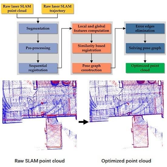
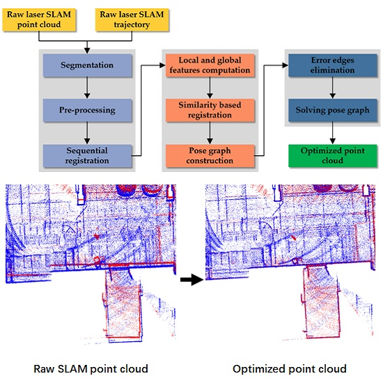
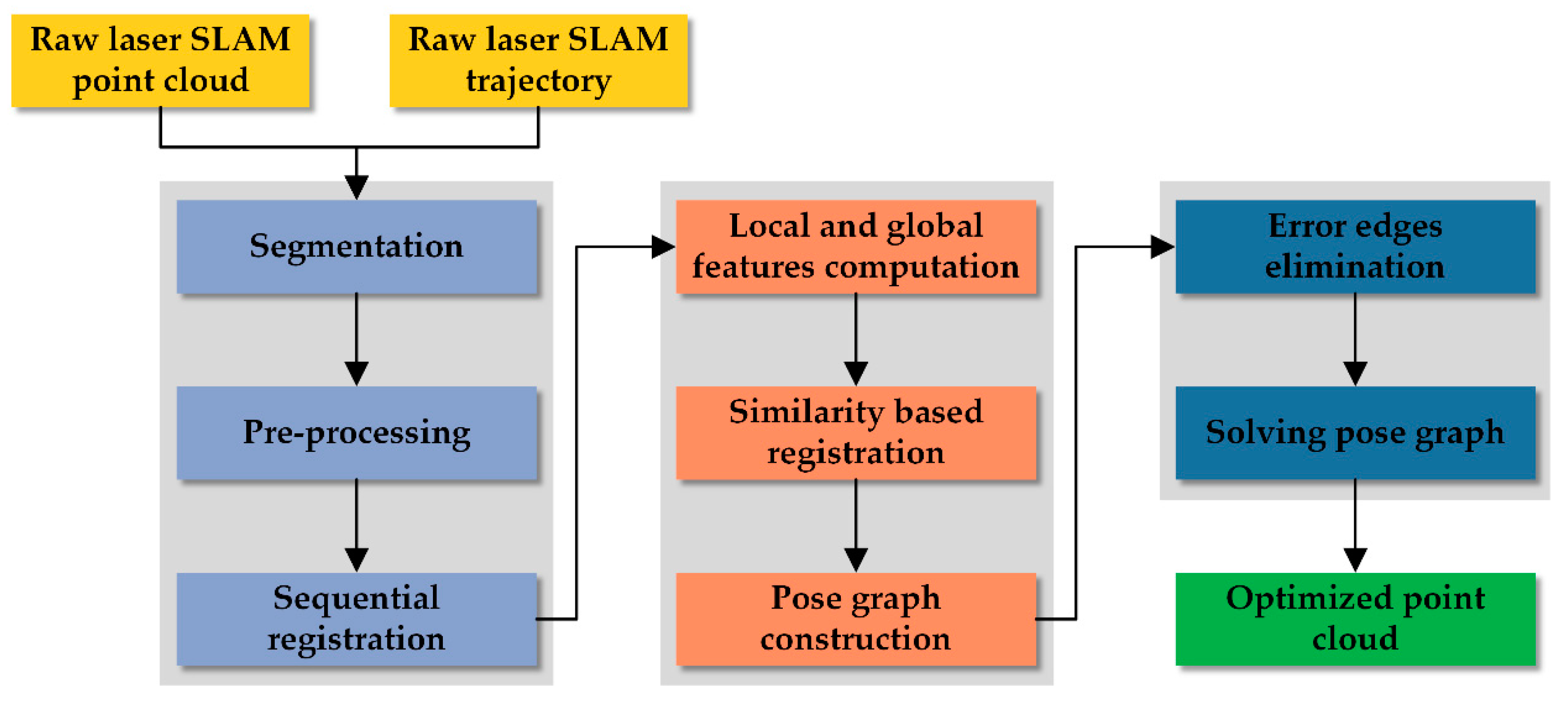
Figure 1.
Overview of the proposed laser simultaneous localization and mapping (SLAM) point cloud optimization algorithm.
Figure 1.
Overview of the proposed laser simultaneous localization and mapping (SLAM) point cloud optimization algorithm.
Figure 2.
An example of point-to-plane iterative closest point (ICP) sequential registration result. (a) The raw point cloud generated by the Cartographer algorithm. (b) The local optimized point cloud after sequential registration. This scene is one of five scenes selected from datasets in the test that decides the algorithm and the values of parameters used for sequential registration.
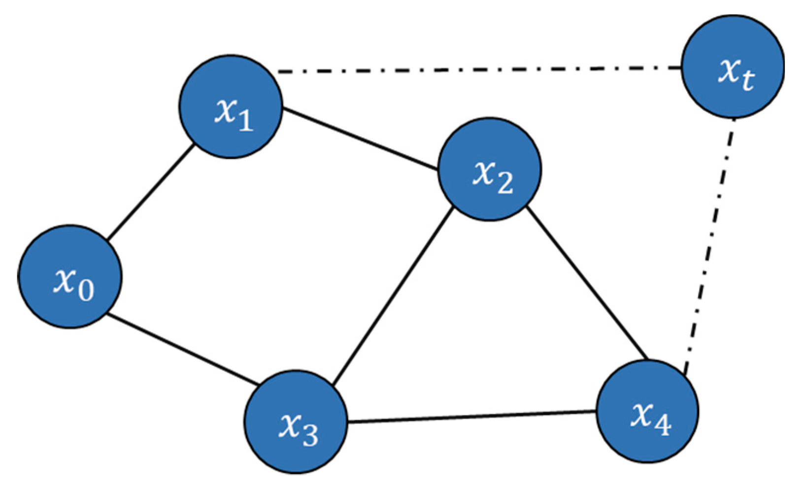
Figure 3.
An example of a pose graph.
Figure 3.
An example of a pose graph.
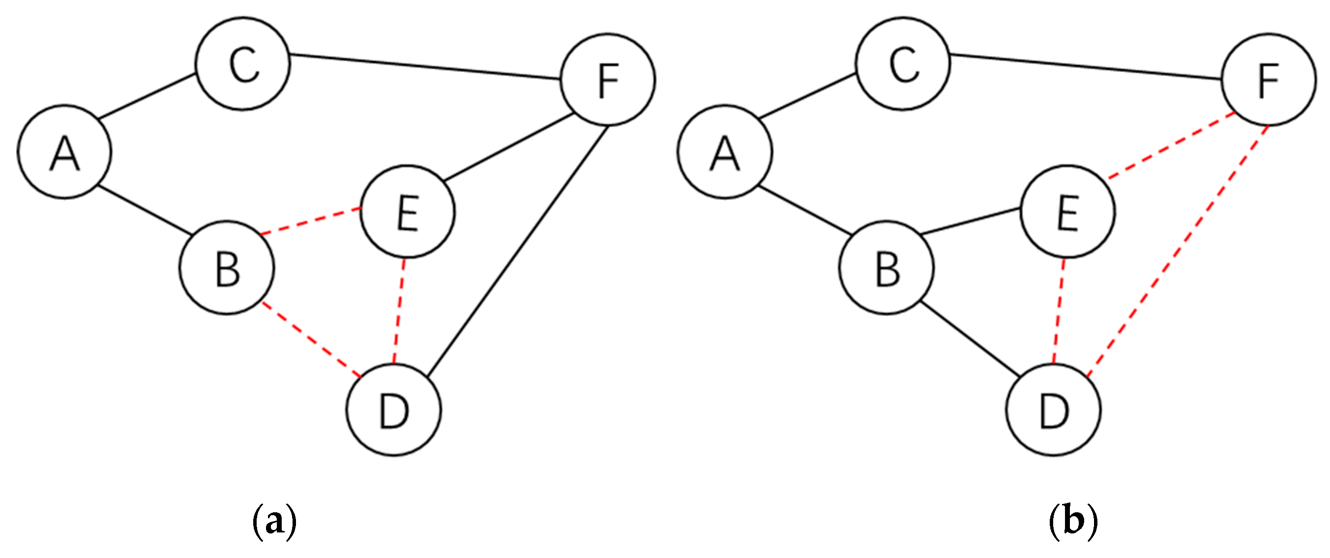
Figure 4.
Fundamental cycle set of an undirected graph. (a) Fundamental cycle set constructed using depth-first search minimal spanning tree; (b) fundamental cycle set constructed using breadth-first search minimal spanning tree. In this figure, black solid lines denote the minimal spanning tree, and the red dotted lines denote missing edges.
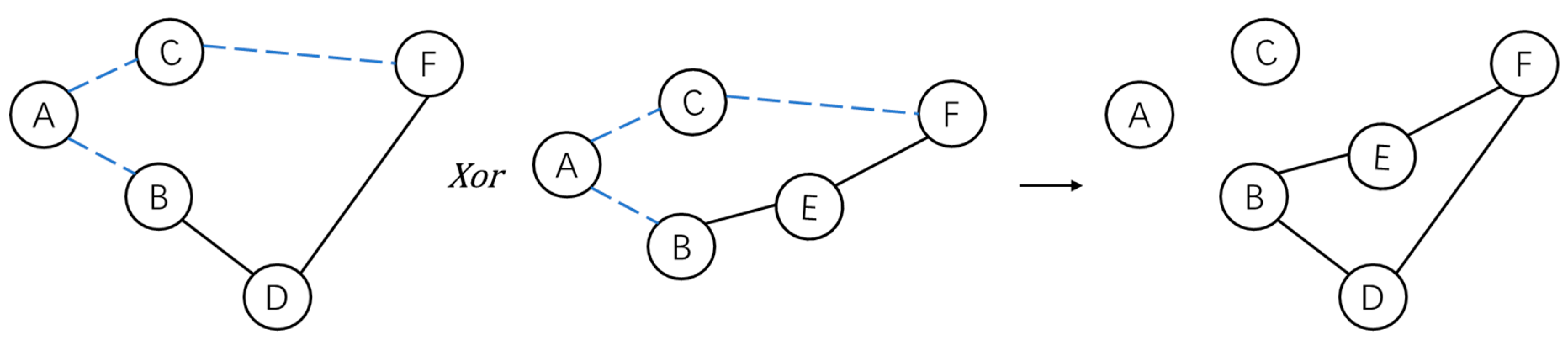
Figure 5.
The illustration of operator . The blue dotted lines denote the edges which are present in both inputs that are removed first, and then the remaining edges and nodes are merged into one.
Figure 5.
The illustration of operator . The blue dotted lines denote the edges which are present in both inputs that are removed first, and then the remaining edges and nodes are merged into one.
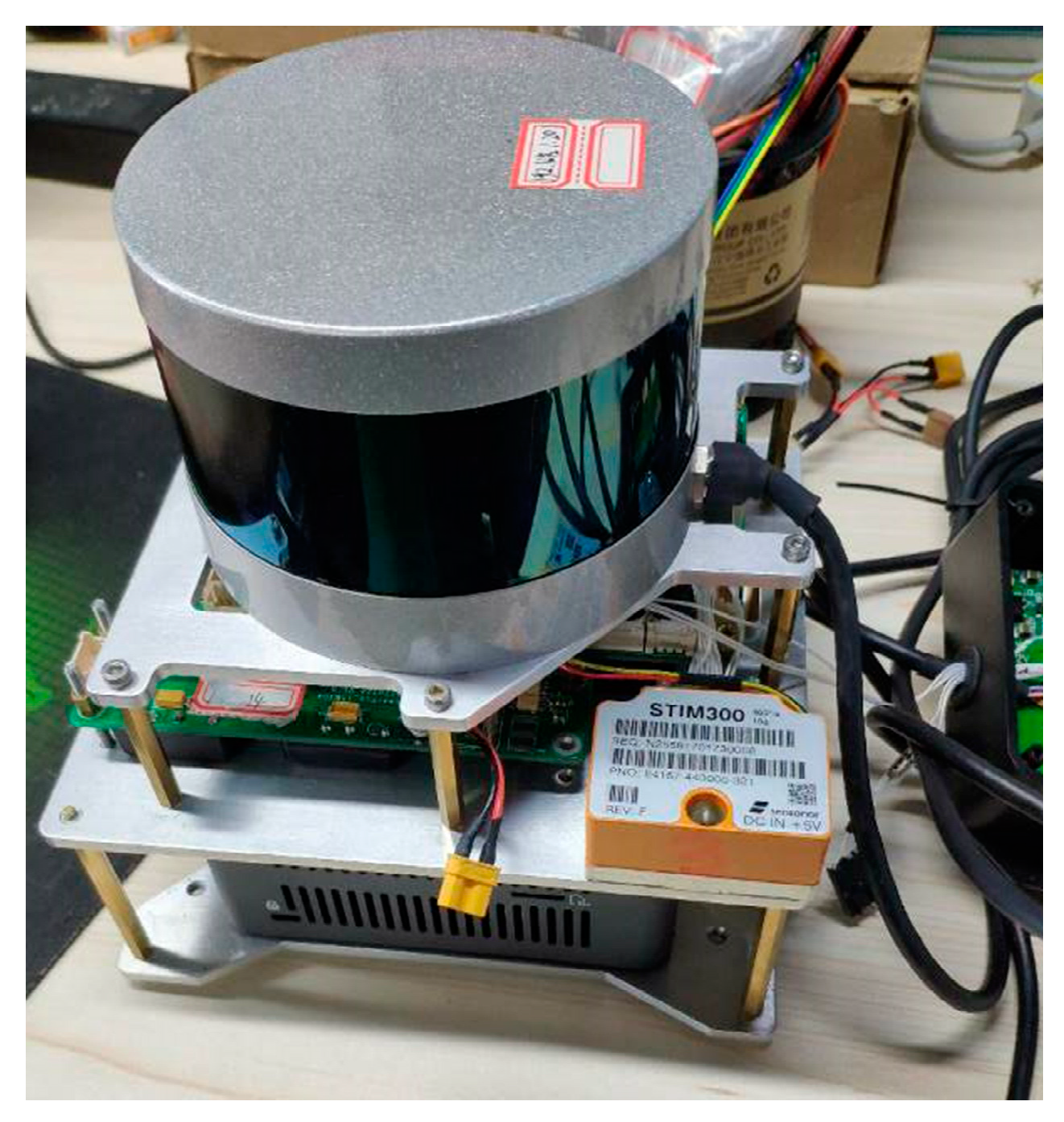
Figure 6.
The hand-held SLAM device description: The laser scanner is Velodyne VLP-16 and the IMU is STIM300. The sensors data are processed by an Intel NUC with Intel Core i7-8559U CPU and 16 GB memory.
Figure 6.
The hand-held SLAM device description: The laser scanner is Velodyne VLP-16 and the IMU is STIM300. The sensors data are processed by an Intel NUC with Intel Core i7-8559U CPU and 16 GB memory.
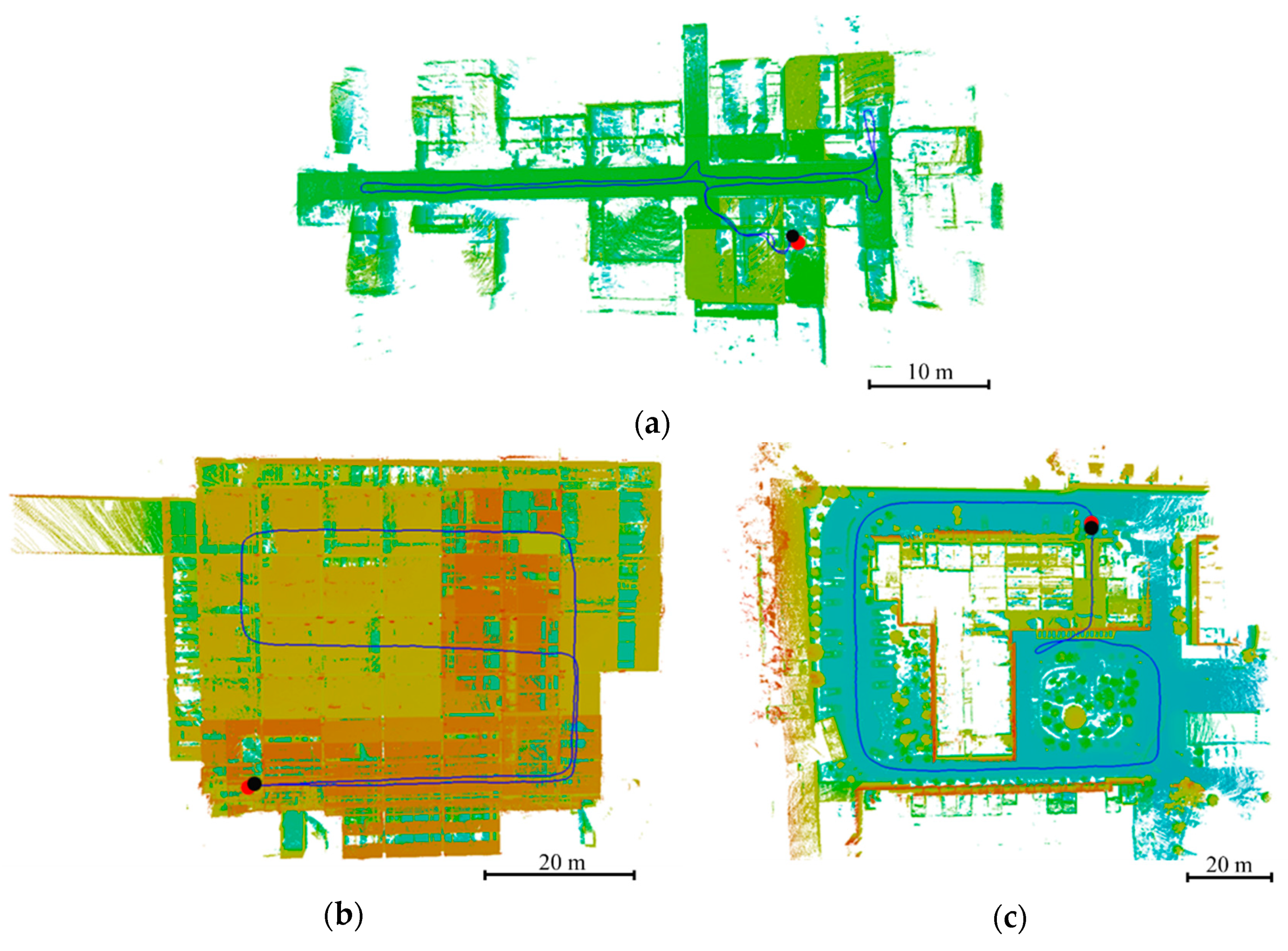
Figure 7.
Experimental environments. (a) Dataset 1; (b) dataset 2; (c) dataset 3.
Figure 7.
Experimental environments. (a) Dataset 1; (b) dataset 2; (c) dataset 3.
Figure 8.
The SLAM device trajectory. The blue line in (a–c) are the trajectories in datasets 1–3 respectively. The red dot and black dot in the figure represent the start and end of trajectory respectively.
Figure 8.
The SLAM device trajectory. The blue line in (a–c) are the trajectories in datasets 1–3 respectively. The red dot and black dot in the figure represent the start and end of trajectory respectively.
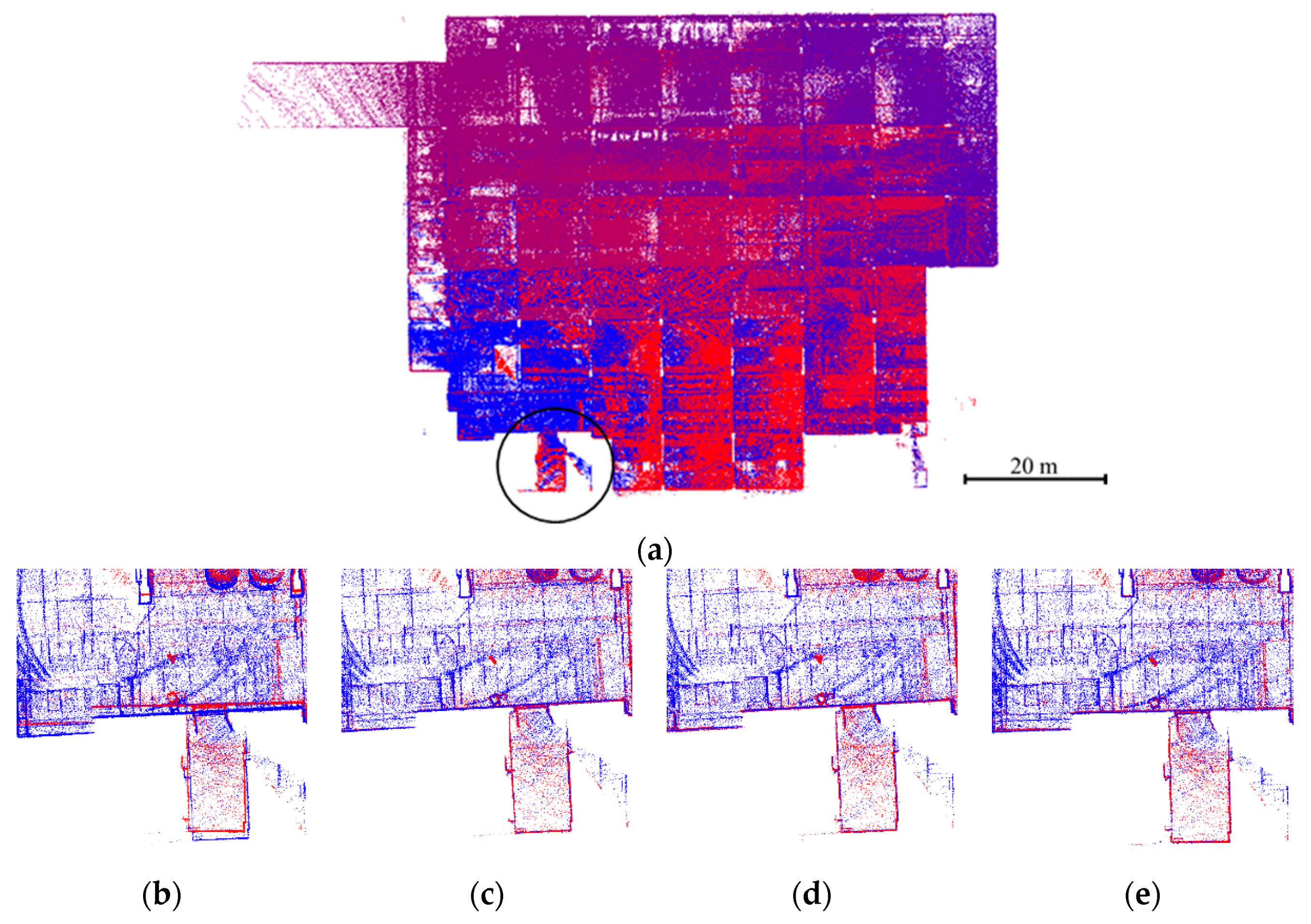
Figure 9.
Comparison between the point clouds before and after optimization in dataset 1. (a) The top view of the point cloud after optimization; (b) enlarged view of the raw output point cloud of Cartographer; (c) enlarged view of the optimized point cloud of Cartographer; (d) enlarged view of the raw output point cloud of lidar odometry and mapping (LOAM); (e) enlarged view of the optimized point cloud of LOAM.
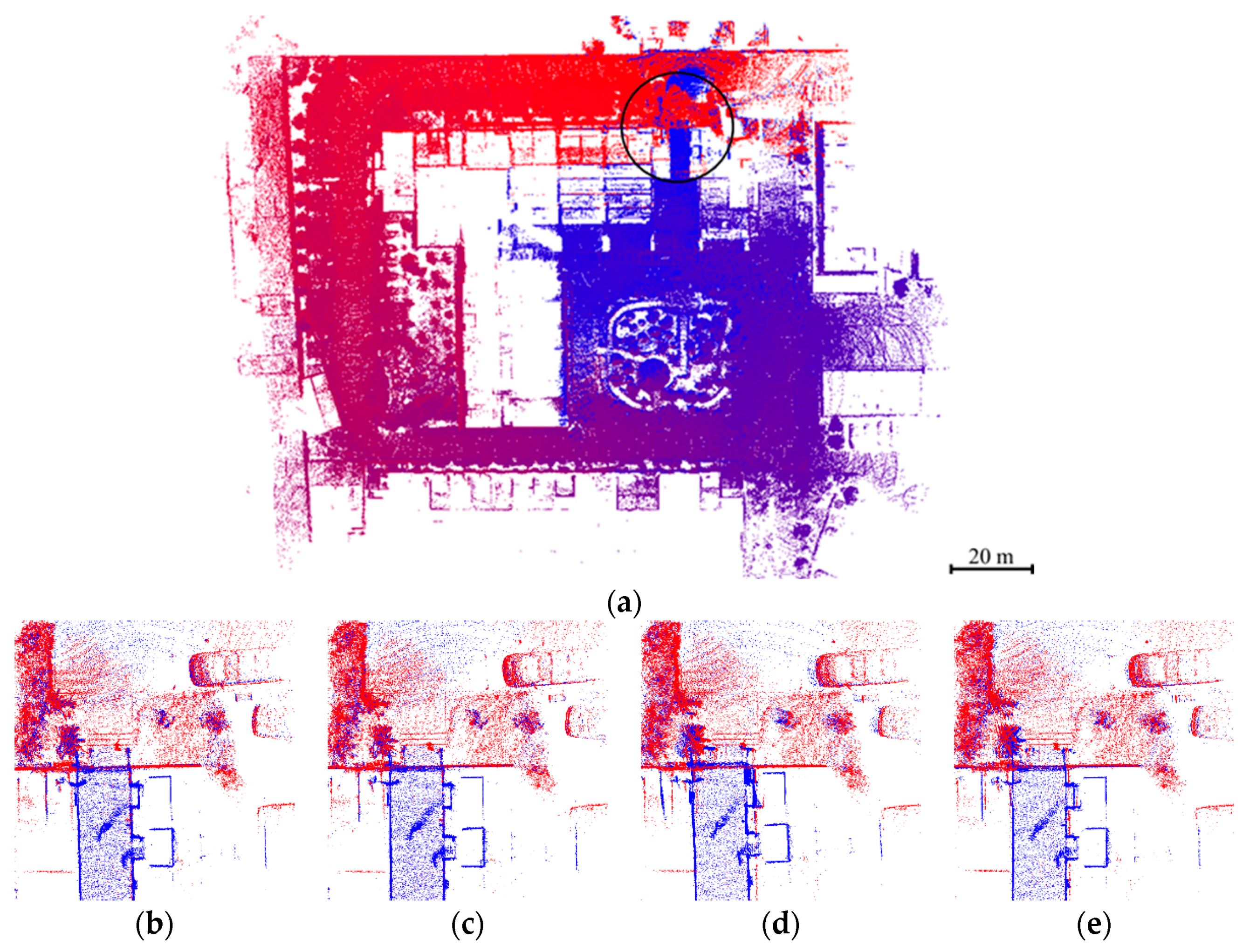
Figure 10.
Comparison between the point clouds before and after optimization in dataset 2. (a) The top view of the point cloud after optimization; (b) enlarged view of the raw output point cloud of Cartographer; (c) enlarged view of the optimized point cloud of Cartographer; (d) enlarged view of the raw output point cloud of LOAM; (e) enlarged view of the optimized point cloud of LOAM.
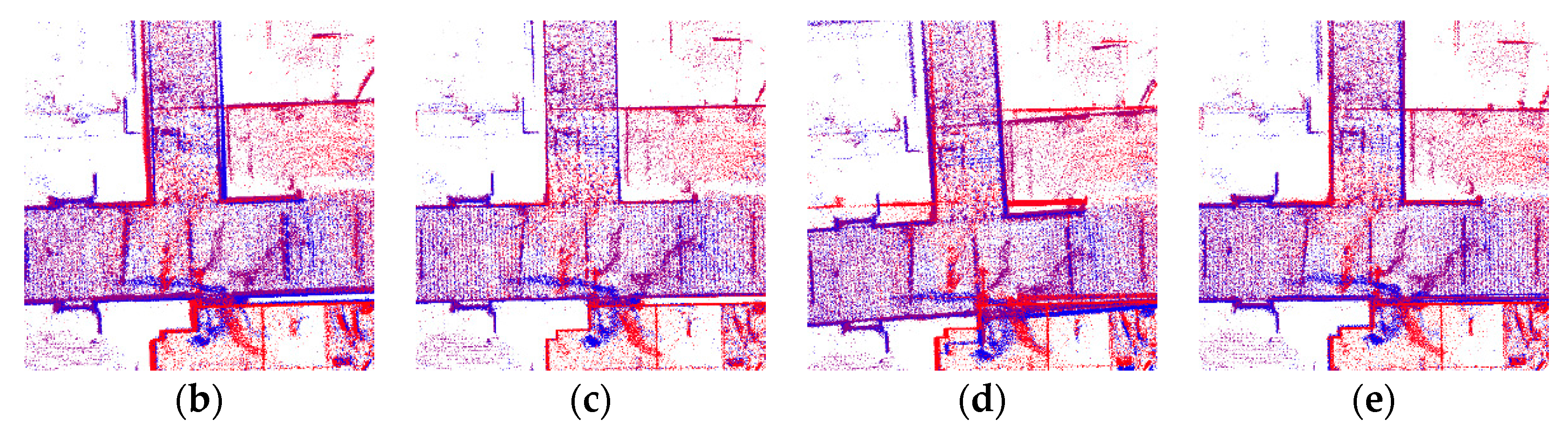
Figure 11.
Comparison between the point clouds before and after optimization in dataset 3. (a) The top view of the point cloud after optimization; (b) enlarged view of the raw output point cloud of Cartographer; (c) enlarged view of the optimized point cloud of Cartographer; (d) enlarged view of the raw output point cloud of LOAM; (e) enlarged view of the optimized point cloud of LOAM.
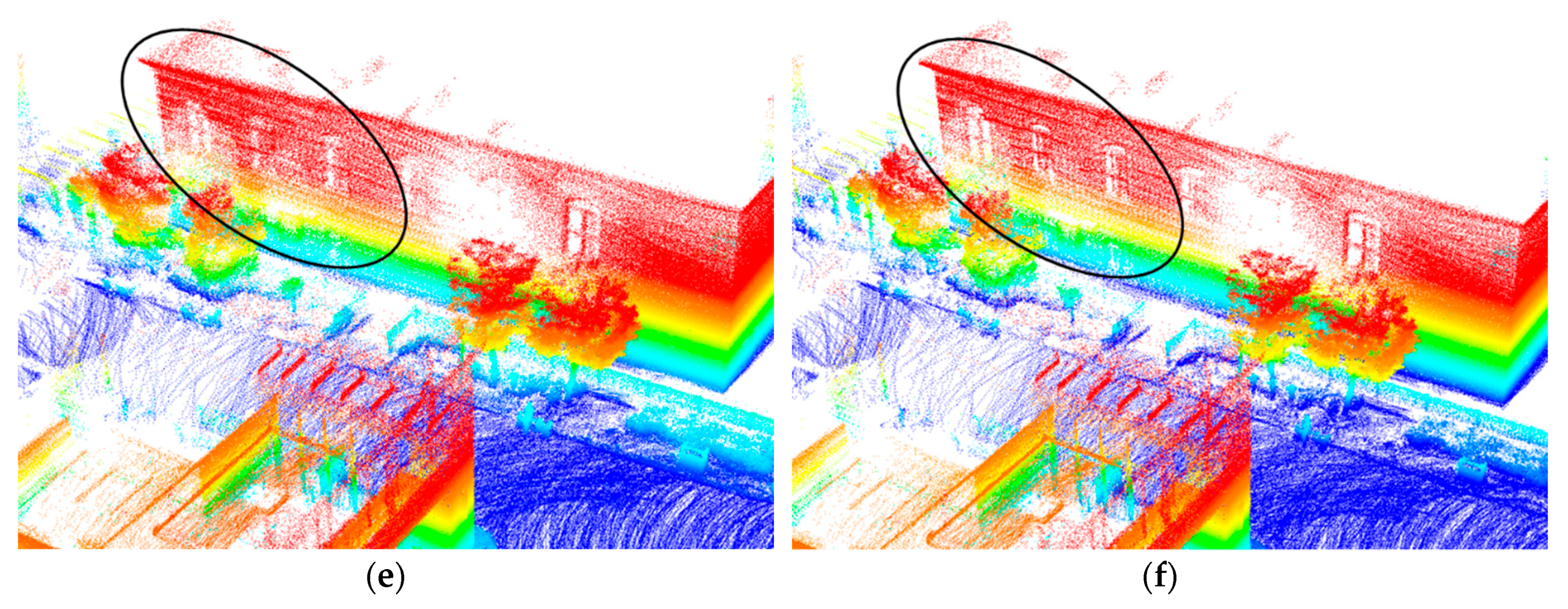
Figure 12.
Snapshots of the point cloud produced by Cartographer before (left) and after optimization (right). (a,b) A scene in dataset 1; (c,d) a scene in dataset 2; (e,f) a scene in dataset 3.
Figure 12.
Snapshots of the point cloud produced by Cartographer before (left) and after optimization (right). (a,b) A scene in dataset 1; (c,d) a scene in dataset 2; (e,f) a scene in dataset 3.
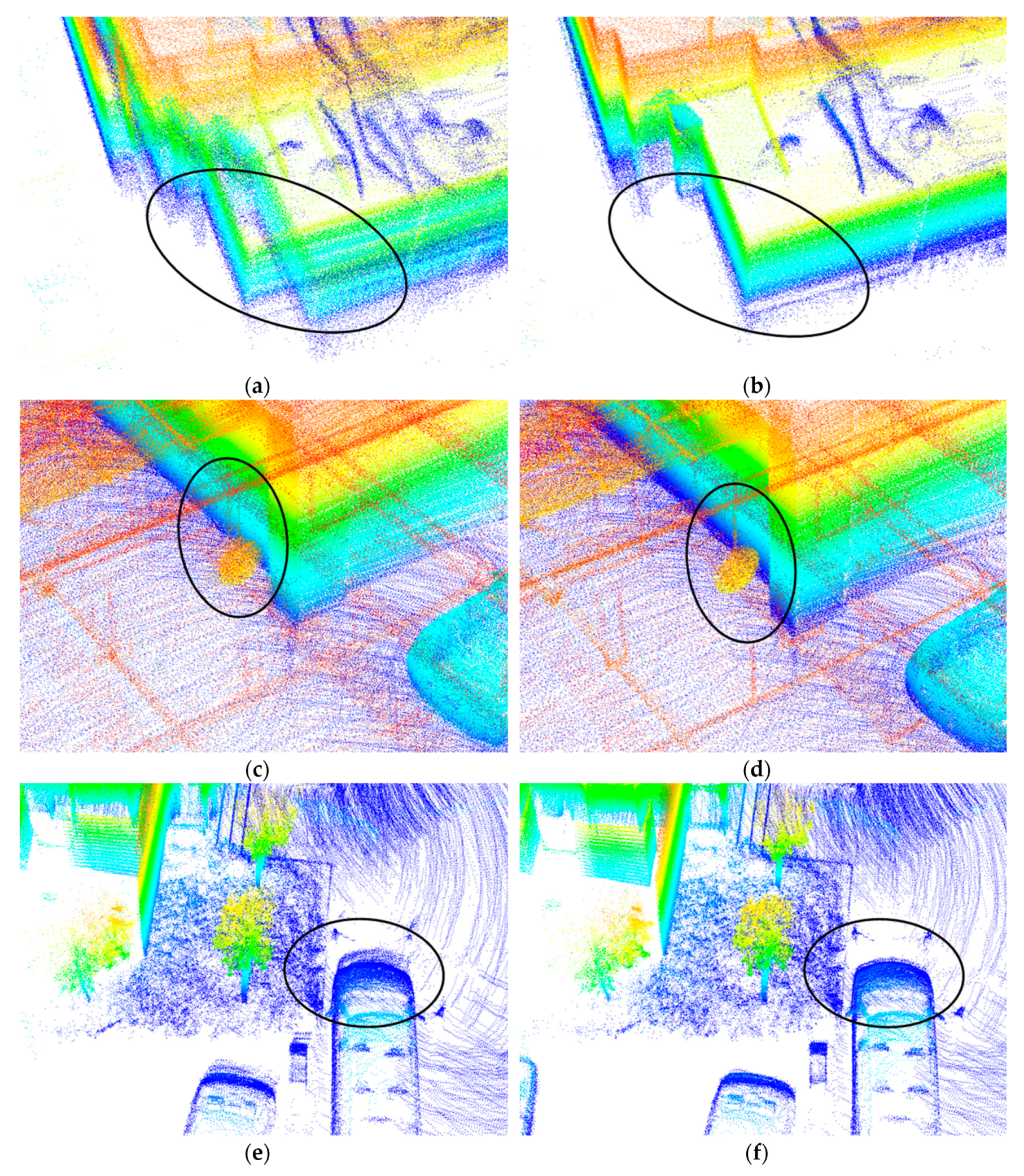
Figure 13.
Snapshots of the point cloud produced by LOAM before (left) and after optimization (right). (a,b) A scene in dataset 1; (c,d) a scene in dataset 2; (e,f) a scene in dataset 3.
Figure 13.
Snapshots of the point cloud produced by LOAM before (left) and after optimization (right). (a,b) A scene in dataset 1; (c,d) a scene in dataset 2; (e,f) a scene in dataset 3.
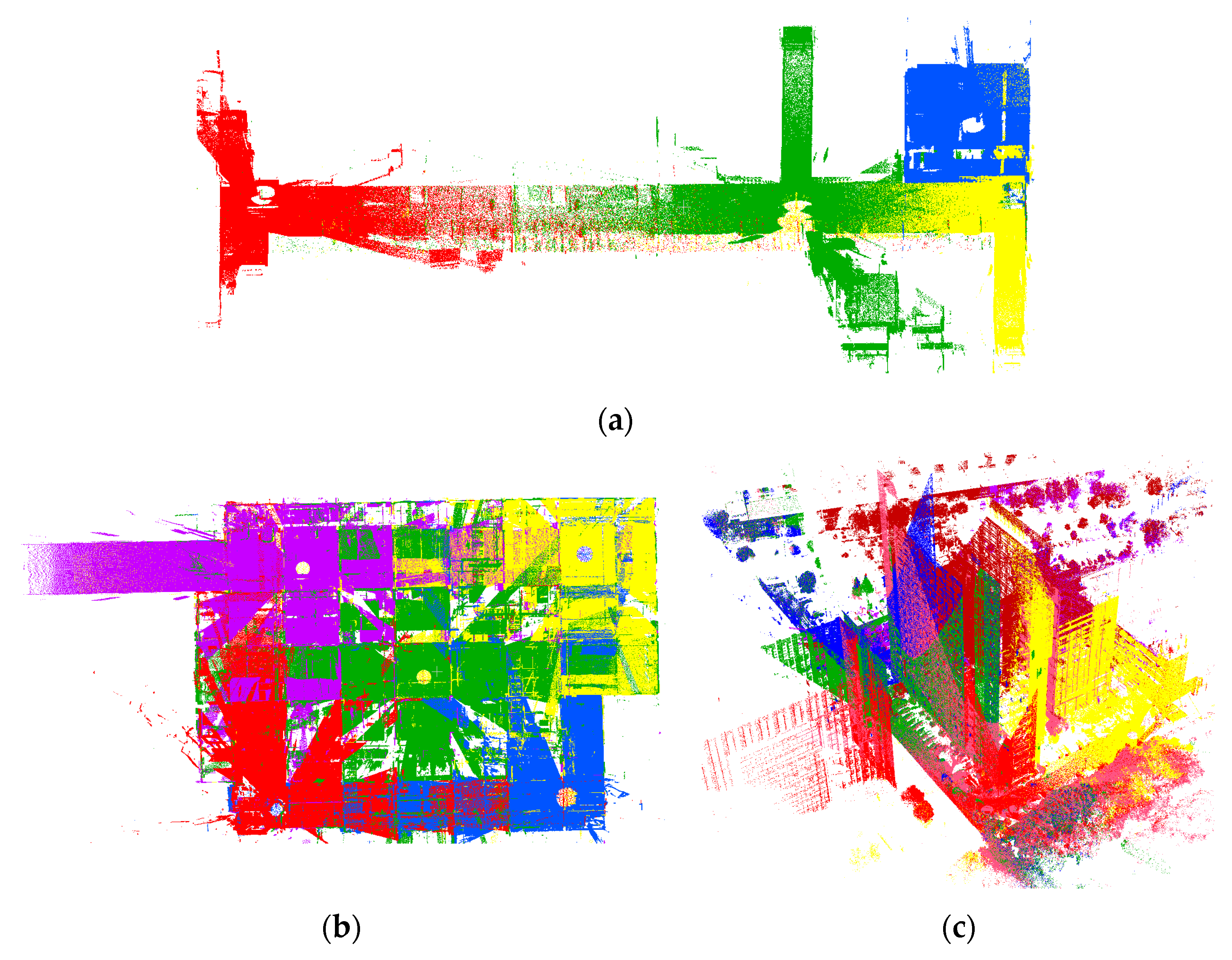
Figure 14.
Overview of the reference data. All scans are rendered by different colors. (a) Dataset 1; (b) dataset 2; (c) dataset 3.
Figure 14.
Overview of the reference data. All scans are rendered by different colors. (a) Dataset 1; (b) dataset 2; (c) dataset 3.
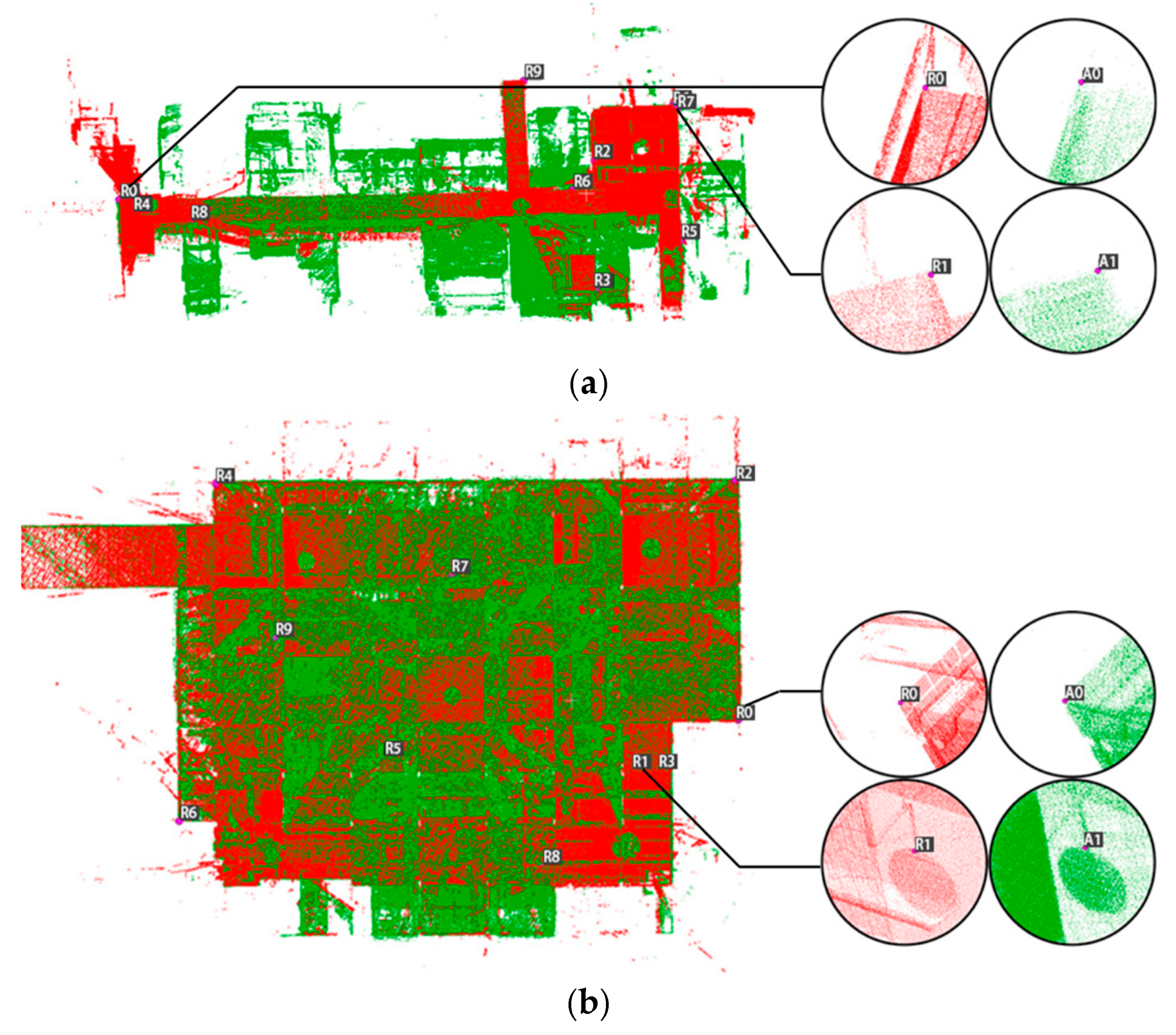
Figure 15.
The distribution of corresponding point pairs in each dataset. The color of the terrestrial laser scanning (TLS) point is red, and the color of the SLAM point is green in the figure. (a) Dataset 1; (b) dataset 2; (c) dataset 3.
Figure 15.
The distribution of corresponding point pairs in each dataset. The color of the terrestrial laser scanning (TLS) point is red, and the color of the SLAM point is green in the figure. (a) Dataset 1; (b) dataset 2; (c) dataset 3.
Figure 16.
Pose graph visualization result. (a) Pose graph of LOAM result in dataset 1; (b) pose graph of LOAM result in dataset 2; (c) pose graph of LOAM result in dataset 3.
Figure 16.
Pose graph visualization result. (a) Pose graph of LOAM result in dataset 1; (b) pose graph of LOAM result in dataset 2; (c) pose graph of LOAM result in dataset 3.
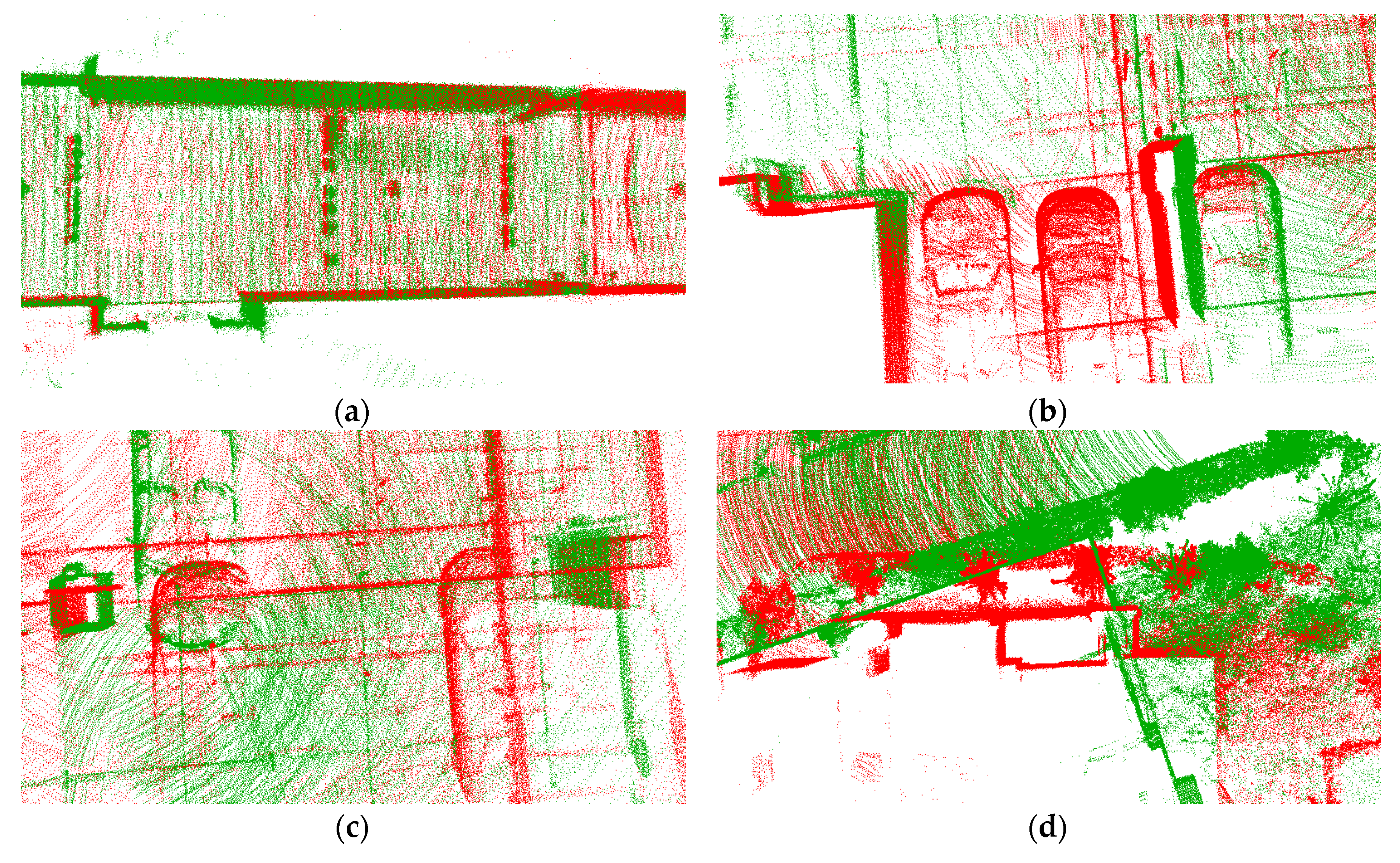
Figure 17.
Examples of registration results corresponding to error edges in the pose graph. (
a) Registration result corresponds to edge 1 in
Figure 16; (
b) registration result corresponds to edge 2 in
Figure 16; (
c) registration result corresponds to edge 3 in
Figure 16; (
d) registration result corresponds to edge 4 in
Figure 16.
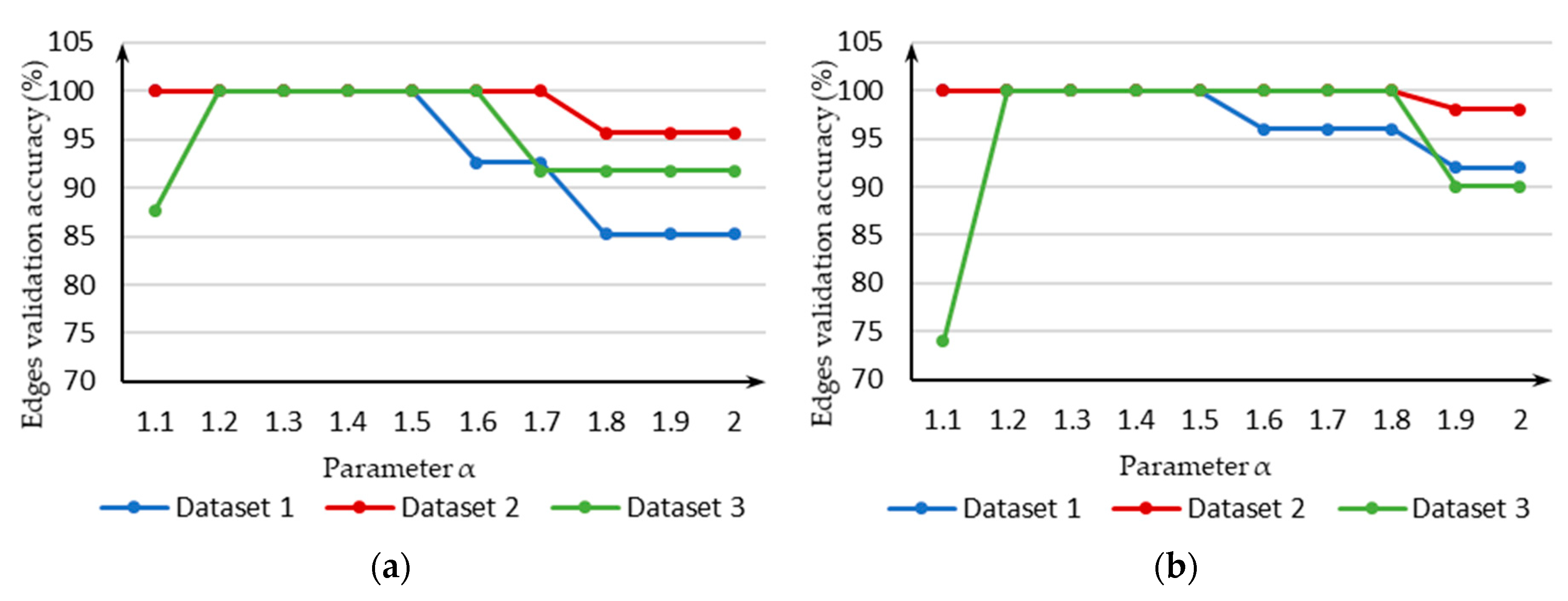
Figure 18.
The edge validation results with different values of parameter α. (a) the results of datasets with the Cartographer algorithm; (b) the results of datasets with the LOAM algorithm.
Figure 18.
The edge validation results with different values of parameter α. (a) the results of datasets with the Cartographer algorithm; (b) the results of datasets with the LOAM algorithm.
Figure 19.
The data acquisition trajectory. The blue line is the trajectory. The red dot and black dot in the figure represent the start and end of trajectory respectively.
Figure 19.
The data acquisition trajectory. The blue line is the trajectory. The red dot and black dot in the figure represent the start and end of trajectory respectively.
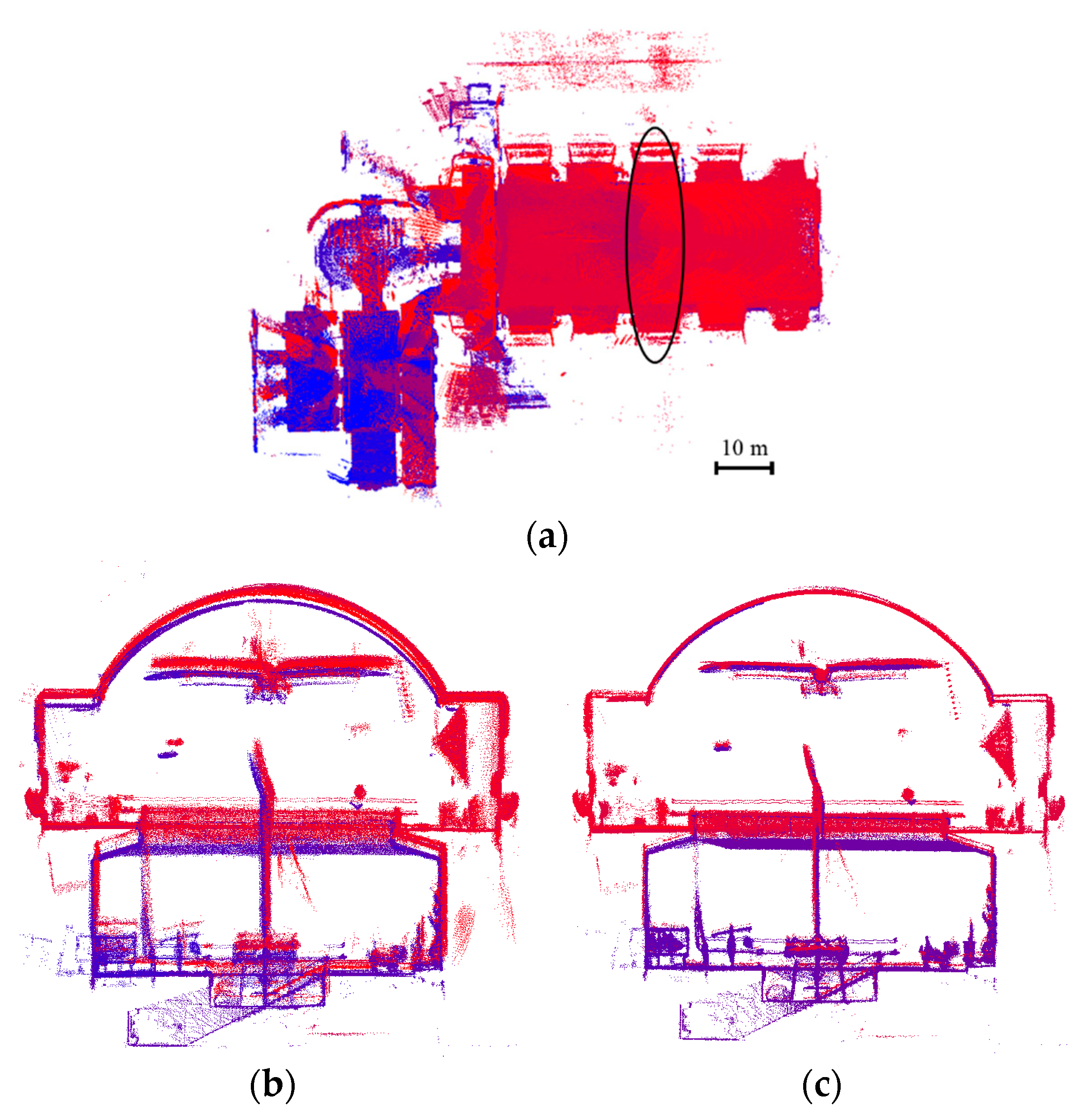
Figure 20.
Comparison between the point clouds before and after optimization in the Cartographer dataset. (
a) The top view of the point cloud after optimization; (
b) section view of the raw output point cloud; (
c) section view of the optimized point cloud. The color render mode is same as
Figure 13.
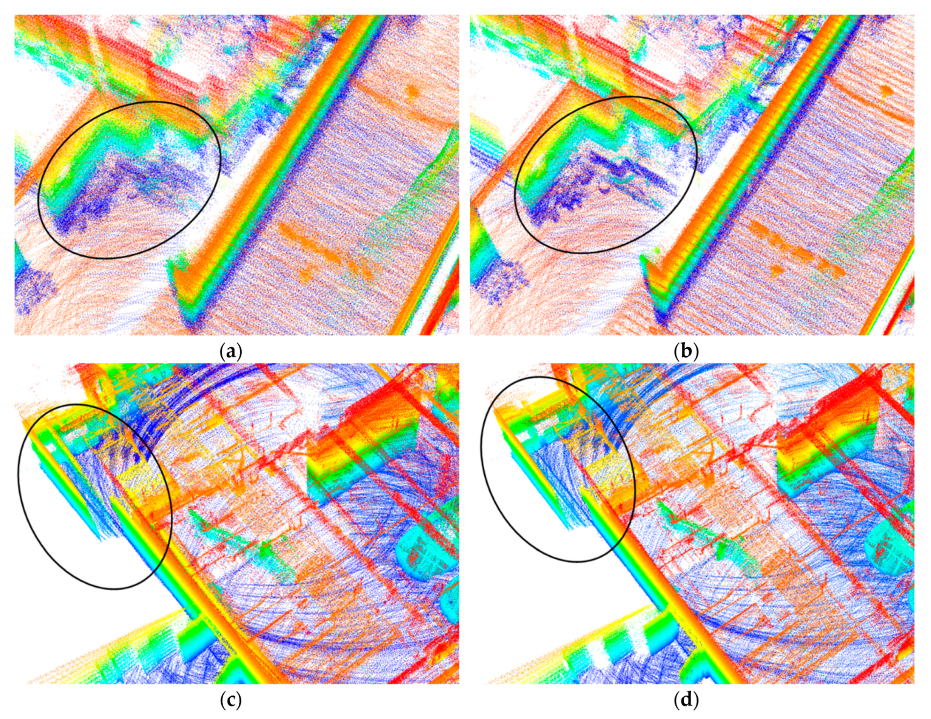
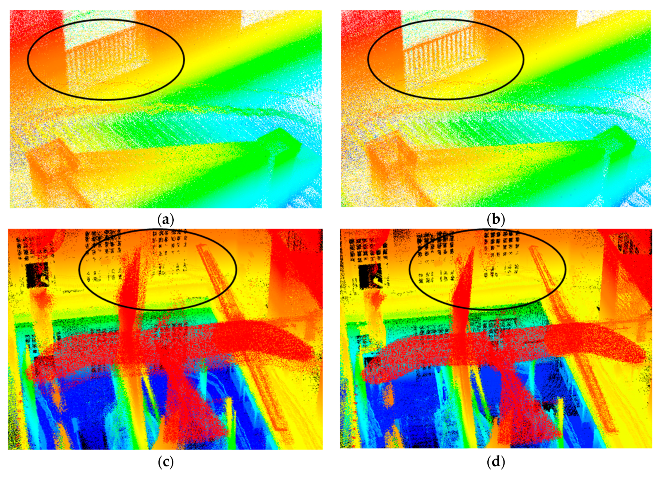
Figure 21.
Snapshots of the point cloud of Cartographer dataset before (left) and after optimization (right). (a,c) the point clouds before optimization; (b,d) the point clouds after optimization.
Figure 21.
Snapshots of the point cloud of Cartographer dataset before (left) and after optimization (right). (a,c) the point clouds before optimization; (b,d) the point clouds after optimization.
Table 1.
Experimental data collection time and trajectory length.
Table 1.
Experimental data collection time and trajectory length.
| Dataset | Time (s) | Trajectory Length (m) |
|---|
| Dataset 1 | 184.4 | 130.9 |
| Dataset 2 | 278.1 | 245.5 |
| Dataset 3 | 283.6 | 286.8 |
Table 2.
Overview of the parameters applied in optimization.
Table 2.
Overview of the parameters applied in optimization.
| | Parameters | Value |
|---|
| Local optimization | Time interval | 10 s |
| Maximum distance | 30 m |
| Sliding window size | 10 |
| Number of neighbors | 20 |
| Voxel resolution | 0.1 m |
| Pose graph construction | Salient radius | 0.3 m |
| Non maxima radius | 0.2 m |
| Sphere radius | 0.5 m |
| Top n similar segment pairs | 3 |
| Global optimization | Residual consistency threshold | 1.2 |
| Maximum iteration | 500 |
Table 3.
The RMSE estimation result of datasets. For the raw output point cloud of LOAM is distorted severely in dataset 1, the initial RMSE values are empty.
Table 3.
The RMSE estimation result of datasets. For the raw output point cloud of LOAM is distorted severely in dataset 1, the initial RMSE values are empty.
| Dataset | Min Distance (m) | | Max Distance (m) | | RMSE (m) |
|---|
| Initial | Optimized | | Initial | Optimized | | Initial | Optimized |
|---|
| Dataset 1 | Cartographer | 0.034 | 0.024 | | 0.180 | 0.100 | 0.109 | 0.064 |
| LOAM | / | 0.052 | | / | 0.227 | / | 0.151 |
| | | | | | | | | |
| Dataset 2 | Cartographer | 0.043 | 0.021 | | 0.348 | 0.097 | 0.158 | 0.059 |
| LOAM | 0.035 | 0.023 | | 0.134 | 0.094 | 0.095 | 0.062 |
| | | | | | | | | |
| Dataset 3 | Cartographer | 0.071 | 0.057 | | 0.210 | 0.124 | 0.154 | 0.102 |
| LOAM | 0.095 | 0.068 | | 0.422 | 0.185 | 0.277 | 0.125 |
Table 4.
The plane-to-plane distance estimation result of datasets. For the raw output point cloud of LOAM is distorted severely in dataset 1, the initial values are empty.
Table 4.
The plane-to-plane distance estimation result of datasets. For the raw output point cloud of LOAM is distorted severely in dataset 1, the initial values are empty.
| Dataset | Min Distance (m) | | Max Distance (m) | | Mean Distance (m) |
|---|
| Initial | Optimized | | Initial | Optimized | | Initial | Optimized |
|---|
| Dataset 1 | Cartographer | 0.037 | 0.012 | | 0.156 | 0.138 | 0.103 | 0.056 |
| LOAM | / | 0.028 | | / | 0.171 | / | 0.074 |
| | | | | | | | | |
| Dataset 2 | Cartographer | 0.021 | 0.016 | | 0.508 | 0.091 | 0.133 | 0.054 |
| LOAM | 0.019 | 0.014 | | 0.170 | 0.103 | 0.084 | 0.050 |
| | | | | | | | | |
| Dataset 3 | Cartographer | 0.028 | 0.022 | | 0.169 | 0. 119 | 0.105 | 0.059 |
| LOAM | 0.034 | 0.024 | | 0.210 | 0.102 | 0.122 | 0.066 |
Table 5.
The time cost of the proposed algorithm.
Table 5.
The time cost of the proposed algorithm.
| Dataset | Local Optimization (s) | Pose Graph Construction (s) | Global Optimization (s) | Total (s) |
|---|
| Dataset 1 | Cartographer | 1033.8 | 56.3 | 12.6 | 1102.7 |
| LOAM | 1167.9 | 63.9 | 12.1 | 1243.9 |
| | | | | | |
| Dataset 2 | Cartographer | 1704.3 | 166.5 | 36.2 | 1907.0 |
| LOAM | 1840.2 | 189.4 | 40.9 | 2070.5 |
| | | | | | |
| Dataset 3 | Cartographer | 1768.4 | 225.3 | 54.5 | 2048.2 |
| LOAM | 1892.2 | 231.1 | 56.7 | 2180 |
Table 6.
Pose graph consistency validation results.
Table 6.
Pose graph consistency validation results.
| Dataset | Nodes | Constructed Edges | Validated Edges | Error Edges |
|---|
| Dataset 1 | Cartographer | 16 | 27 | 25 | 2 |
| LOAM | 16 | 25 | 24 | 1 |
| | | | | | |
| Dataset 2 | Cartographer | 24 | 46 | 40 | 6 |
| LOAM | 24 | 49 | 41 | 8 |
| | | | | | |
| Dataset 3 | Cartographer | 26 | 49 | 45 | 4 |
| LOAM | 26 | 50 | 44 | 6 |
Table 7.
The precision evaluation result of the Cartographer dataset.
Table 7.
The precision evaluation result of the Cartographer dataset.
| | Initial | Optimized |
|---|
| Mean map entropy | −2.86 | −3.04 |
| Mean plane variance (m) | 0.067 | 0.039 |


