Earthquake-Induced Landslide Mapping for the 2018 Hokkaido Eastern Iburi Earthquake Using PALSAR-2 Data


Abstract
1. Introduction
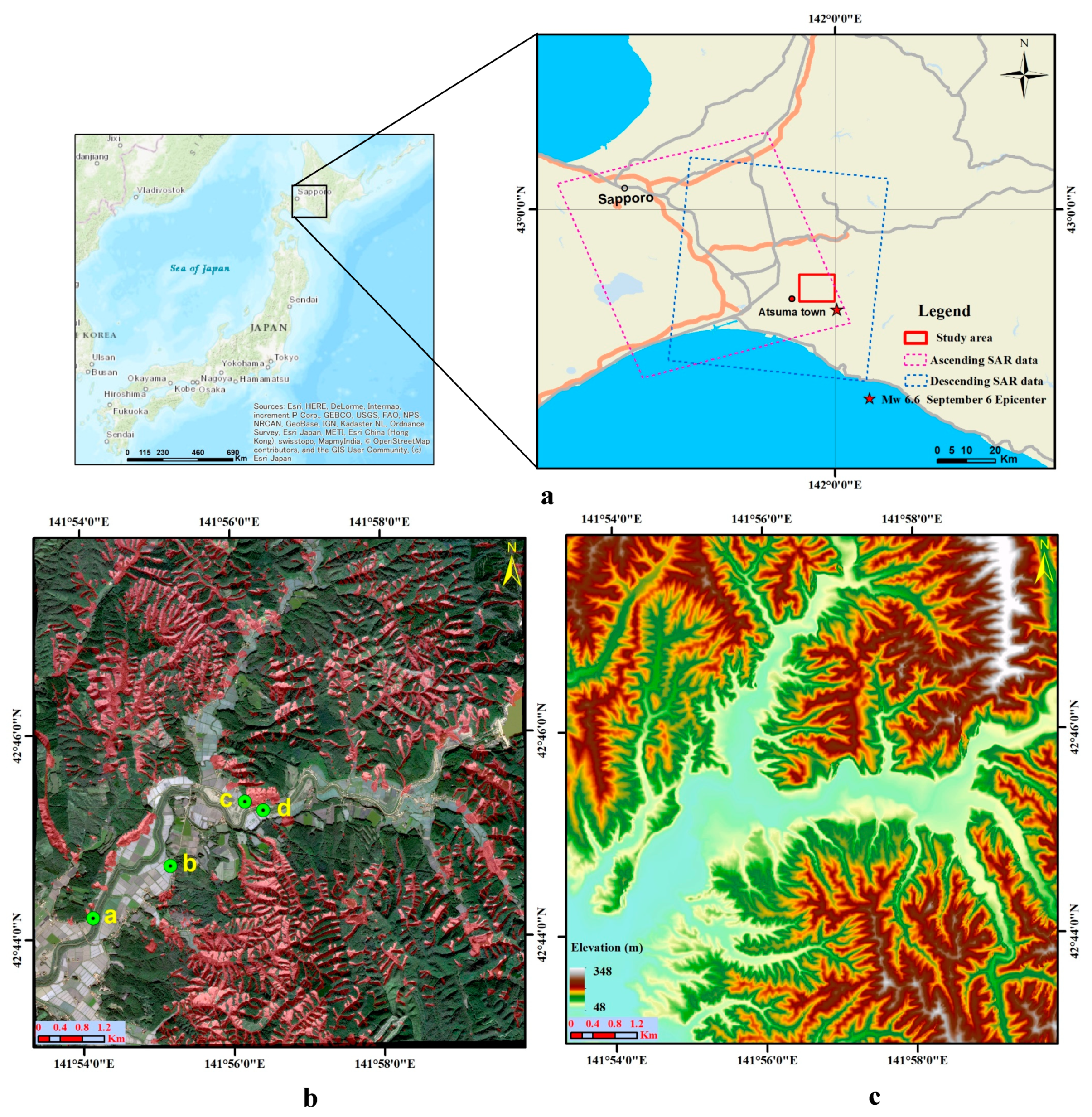
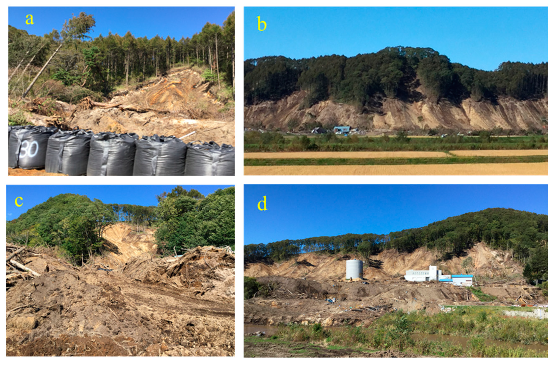
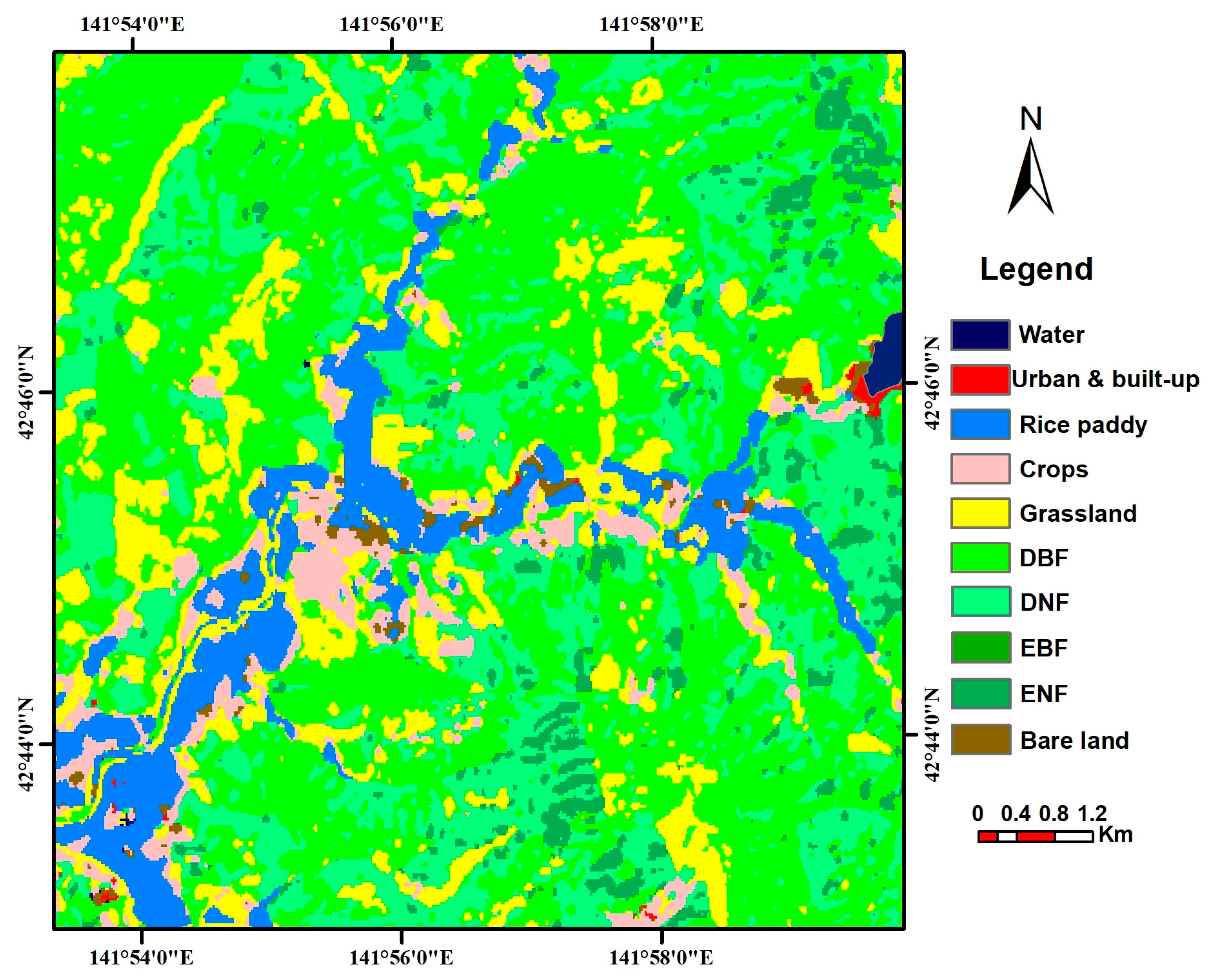
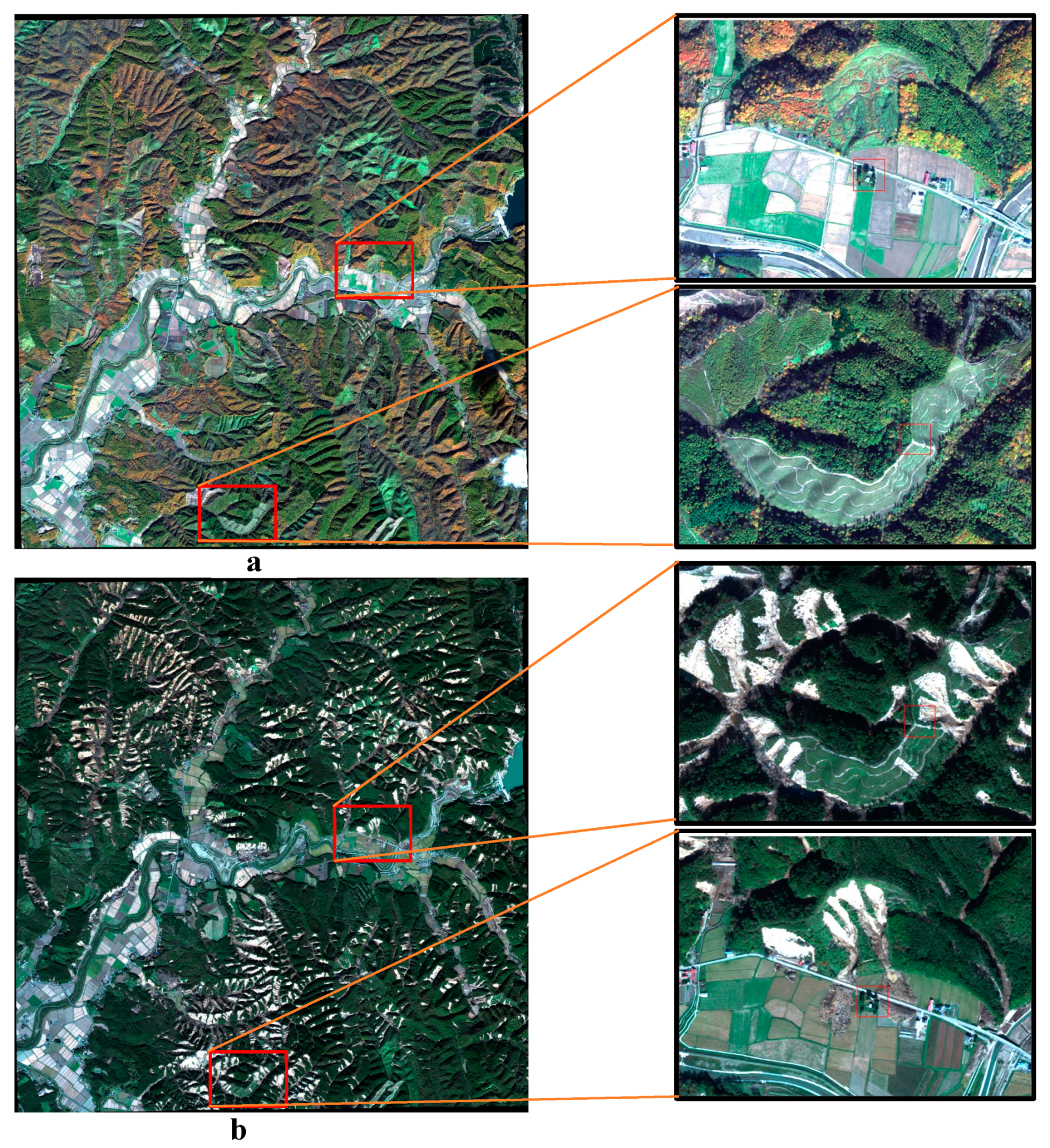
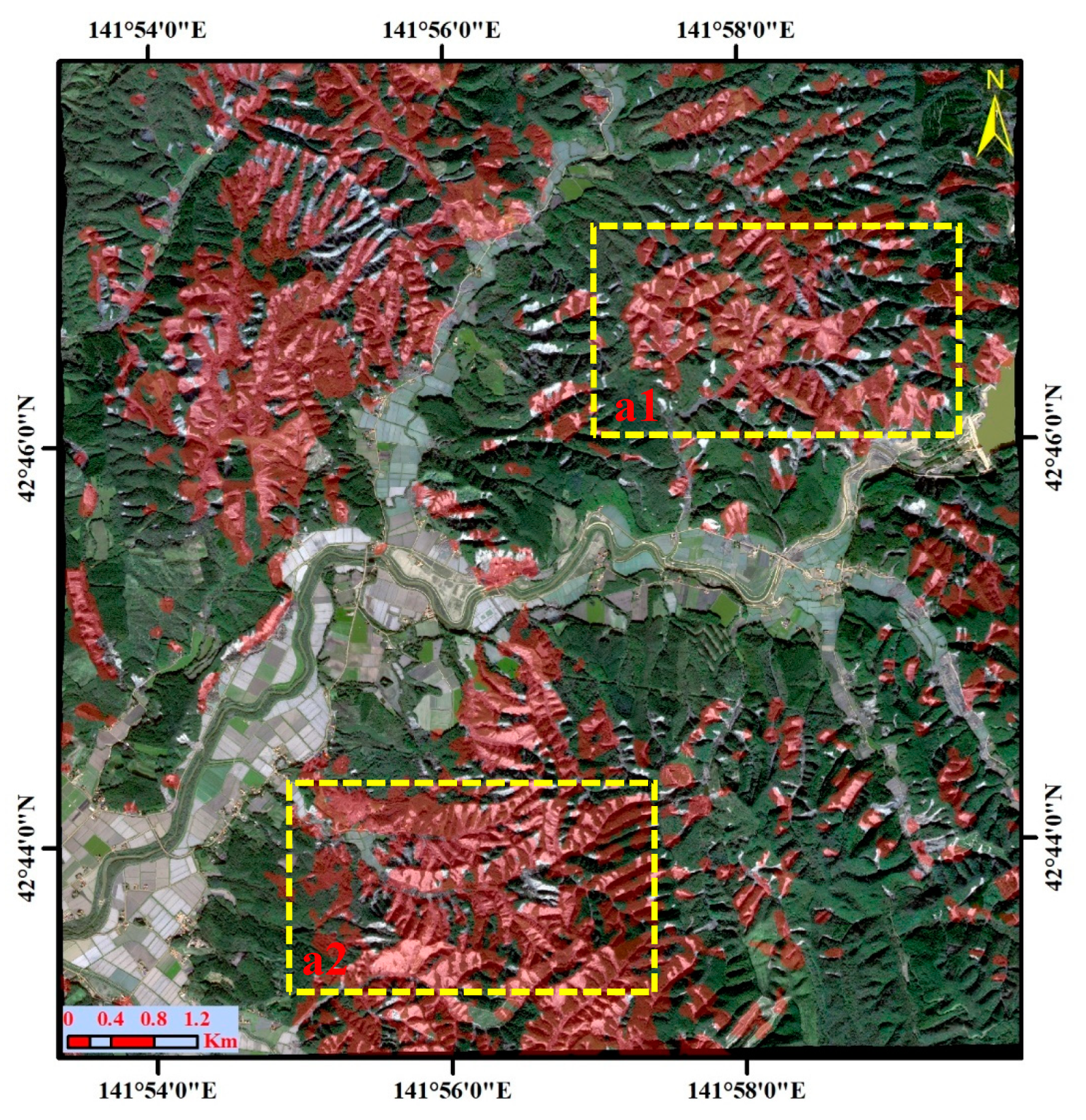
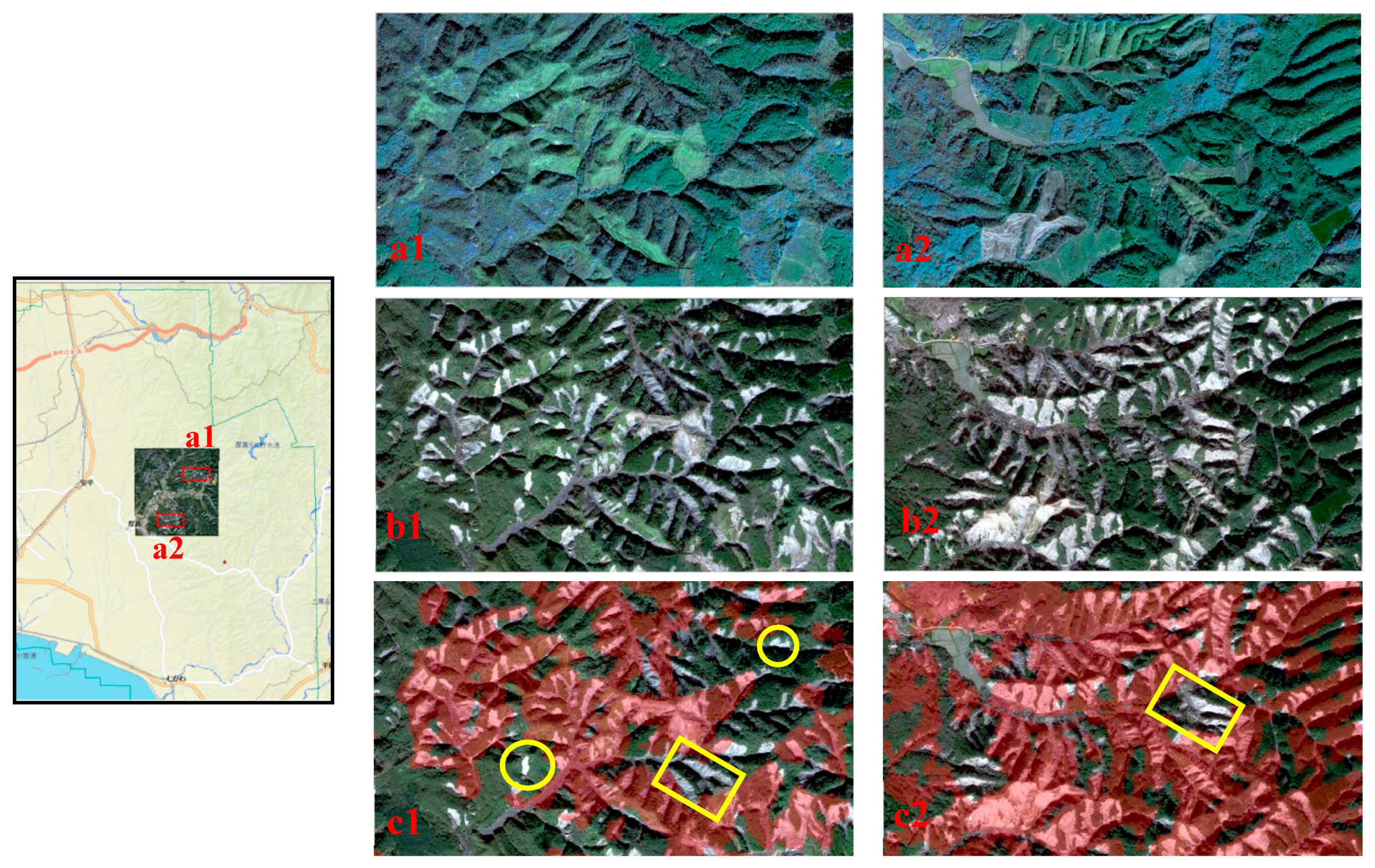
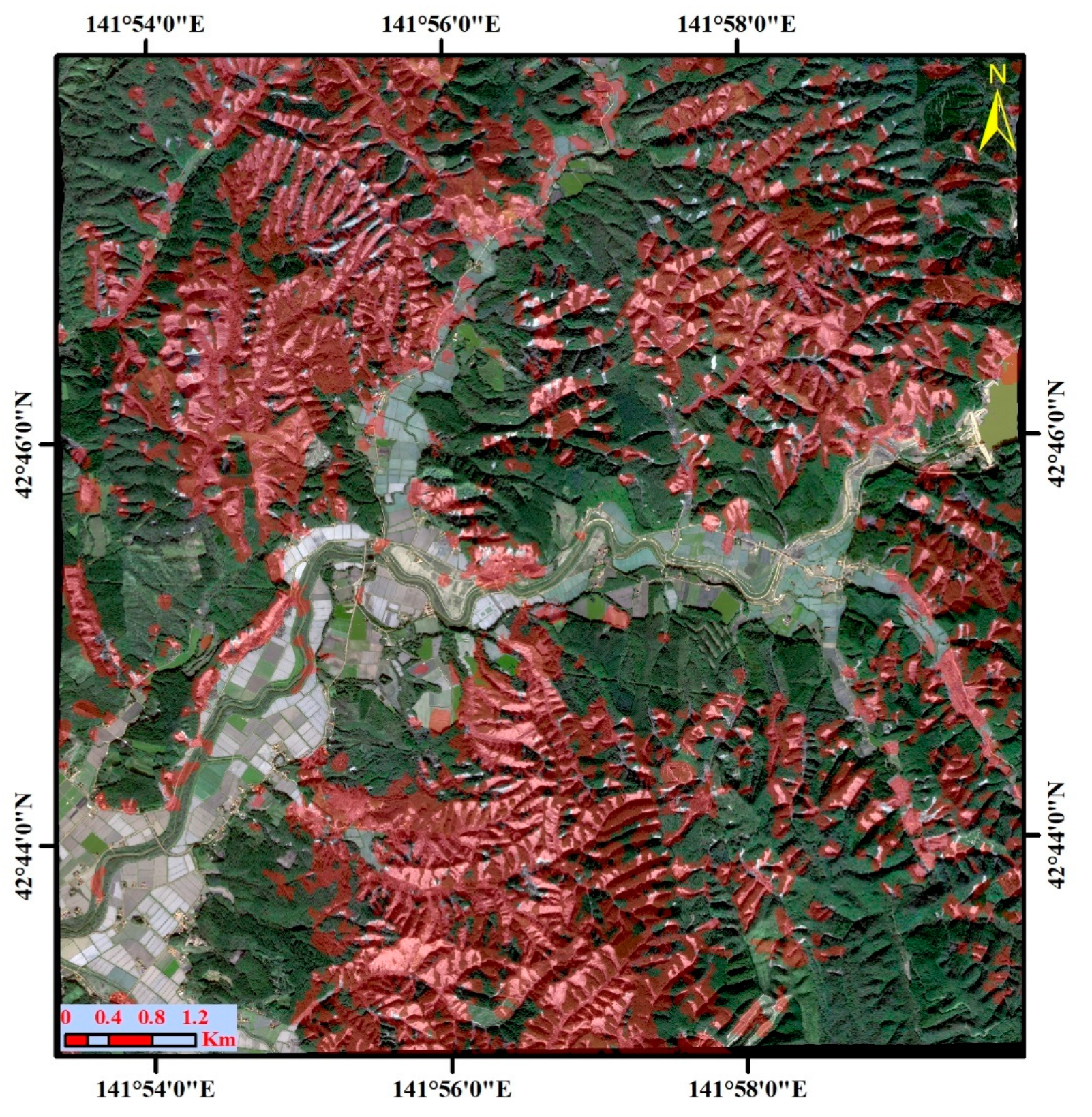
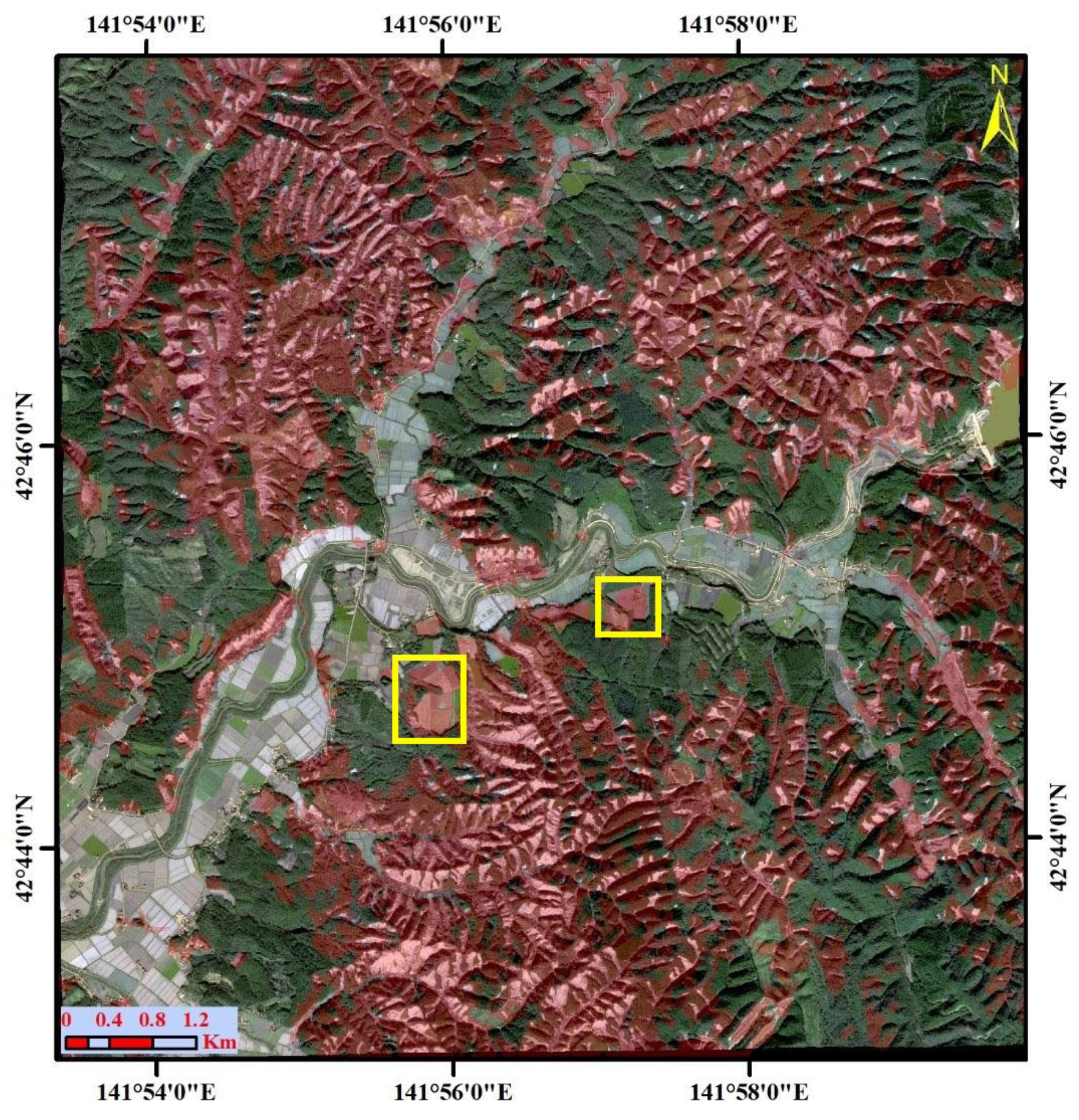
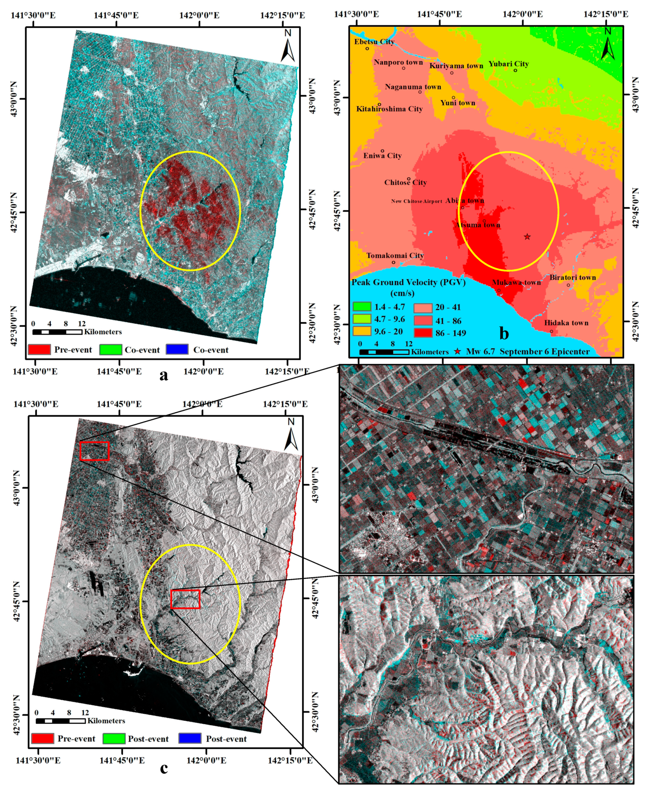
2. Study Area
3. Datasets
4. Methodology
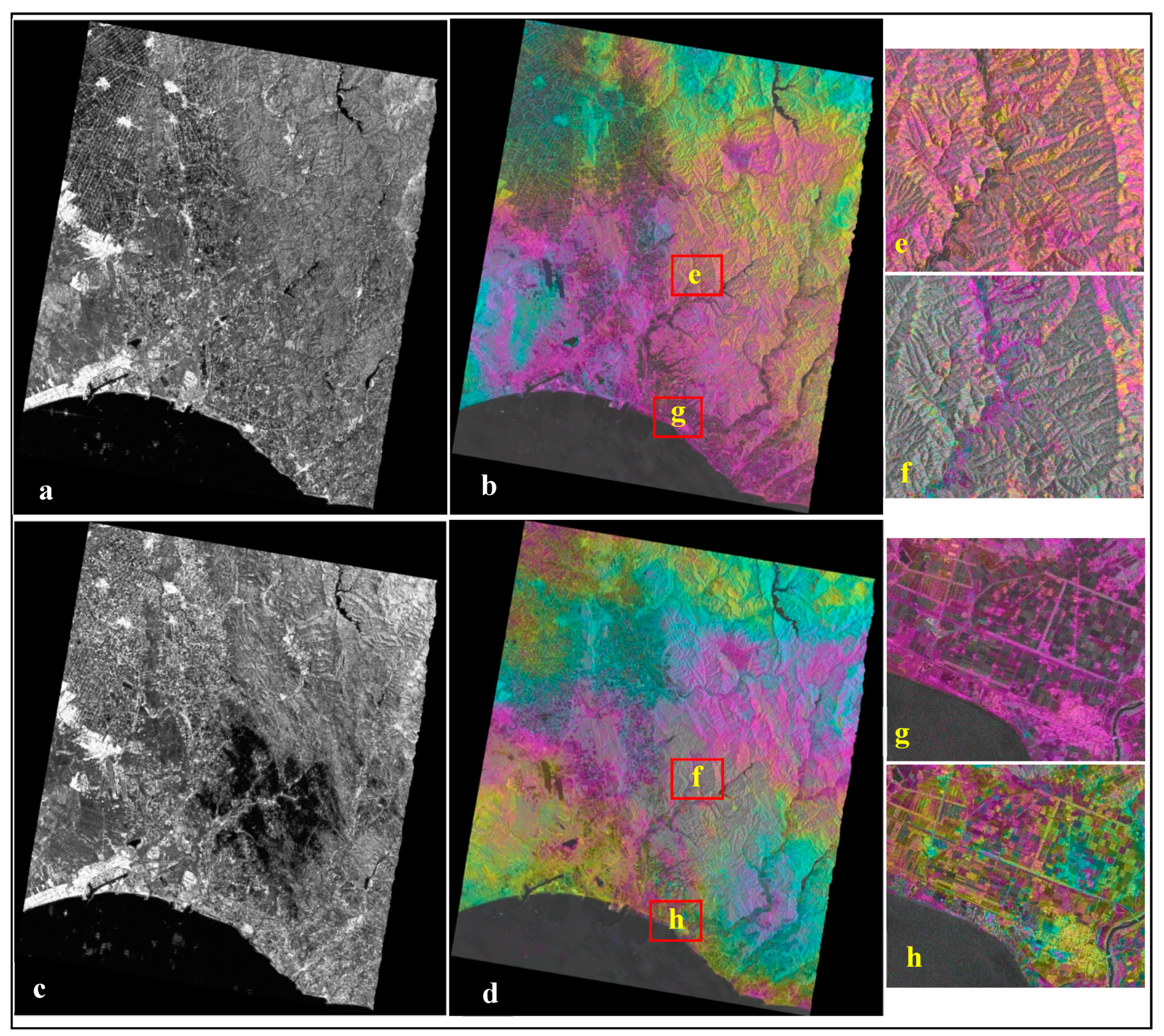
4.1. Synthetic Aperture Radar: Interferometry and Coherence
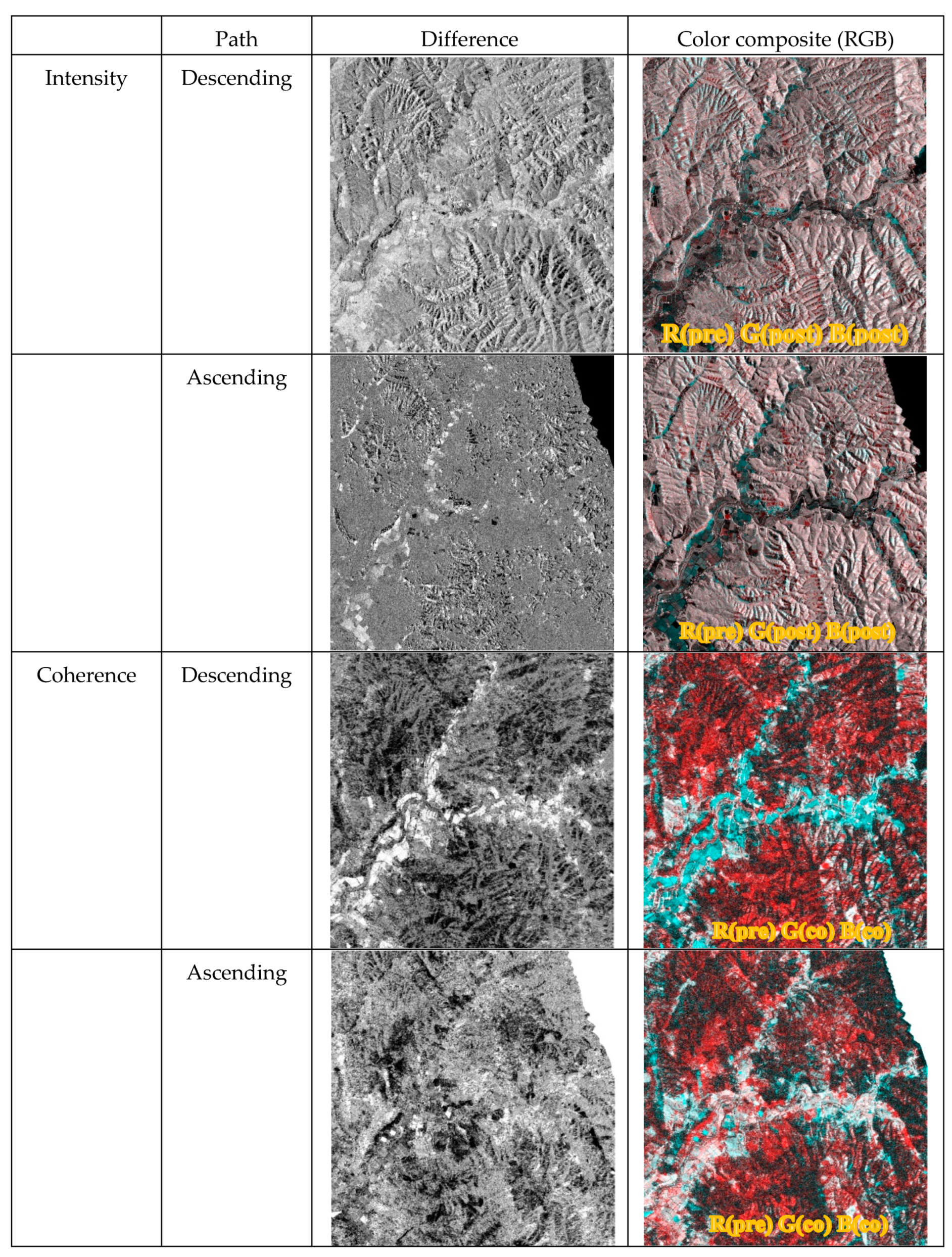
4.2. SAR Coherence and Intensity Difference
4.3. Statistical Methods
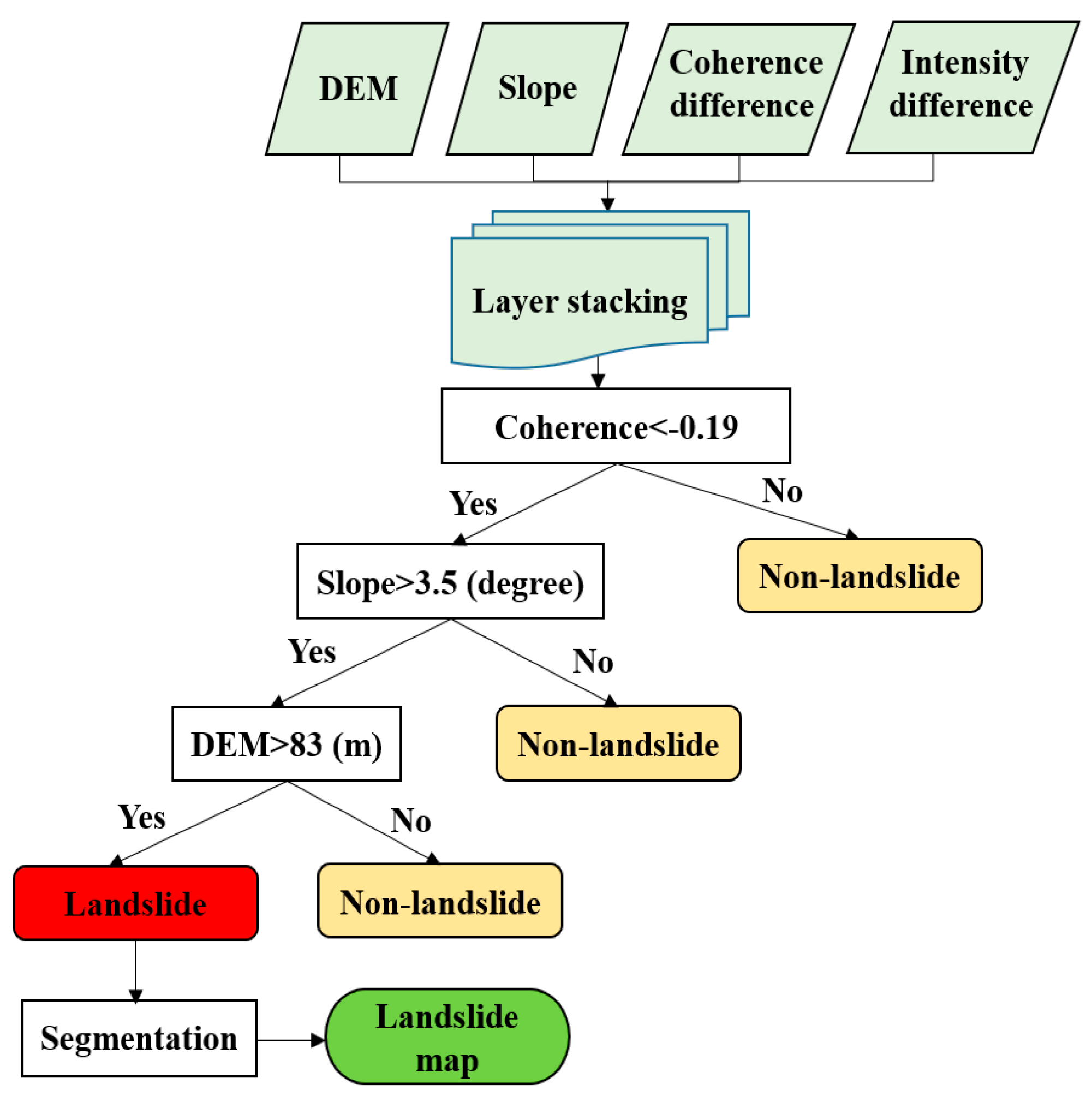
4.4. Decision Tree Classification
5. Results
5.1. Landslide Classification Using Descending and Ascending SAR Images
5.2. Quantitative Analysis of the Landslide Classification Accuracy
6. Discussion
7. Conclusions
Author Contributions
Funding
Acknowledgments
Conflicts of Interest
References
- Roback, K.; Clark, M.K.; West, A.J.; Zekkos, D.; Li, G.; Gallen, S.F.; Chamlagain, D.; Godt, J.W. The size, distribution, and mobility of landslides caused by the 2015 Mw7.8 Gorkha earthquake, Nepal. Geomorphology 2018, 301, 121–138. [Google Scholar] [CrossRef]
- Plank, S. Rapid damage assessment by means of multi-temporal SAR—A comprehensive review and outlook to Sentinel-1. Remote Sens. 2014, 6, 4870–4906. [Google Scholar] [CrossRef]
- Tofani, V.; Segoni, S.; Agostini, A.; Catani, F.; Casagli, N. Technical Note: Use of remote sensing for landslide studies in Europe. Nat. Hazards Earth Syst. Sci. 2013, 13, 299–309. [Google Scholar] [CrossRef]
- Casagli, N.; Frodella, W.; Morelli, S.; Tofani, V.; Ciampalini, A.; Intrieri, E.; Raspini, F.; Rossi, G.; Tanteri, L.; Lu, P. Spaceborne, UAV and ground-based remote sensing techniques for landslide mapping, monitoring and early warning. Geoenviron. Disasters 2017, 4, 9. [Google Scholar] [CrossRef]
- Liu, X.; Zhao, C.; Zhang, Q.; Peng, J.; Zhu, W.; Lu, Z. Multi-temporal loess landslide inventory mapping with C-, X- and L-band SAR datasets-a case study of Heifangtai loess landslides, China. Remote Sens. 2018, 10, 2756. [Google Scholar] [CrossRef]
- Plank, S.; Twele, A.; Martinis, S.; Plank, S.; Twele, A.; Martinis, S. Landslide mapping in vegetated areas using change detection based on optical and polarimetric SAR data. Remote Sens. 2016, 8, 307. [Google Scholar] [CrossRef]
- Burrows, K.; Walters, R.J.; Milledge, D.; Spaans, K.; Densmore, A.L.; Burrows, K.; Walters, R.J.; Milledge, D.; Spaans, K.; Densmore, A.L. A new method for large-scale landslide classification from Satellite Radar. Remote Sens. 2019, 11, 237. [Google Scholar] [CrossRef]
- Strozzi, T.; Ambrosi, C.; Raetzo, H.; Strozzi, T.; Ambrosi, C.; Raetzo, H. Interpretation of aerial photographs and satellite SAR interferometry for the inventory of landslides. Remote Sens. 2013, 5, 2554–2570. [Google Scholar] [CrossRef]
- Bardi, F.; Frodella, W.; Ciampalini, A.; Bianchini, S.; Del Ventisette, C.; Gigli, G.; Fanti, R.; Moretti, S.; Basile, G.; Casagli, N. Integration between ground based and satellite SAR data in landslide mapping: The San Fratello case study. Geomorphology 2014, 223, 45–60. [Google Scholar] [CrossRef]
- Dong, J.; Zhang, L.; Li, M.; Yu, Y.; Liao, M.; Gong, J.; Luo, H. Measuring precursory movements of the recent Xinmo landslide in Mao County, China with Sentinel-1 and ALOS-2 PALSAR-2 datasets. Landslides 2018, 15, 135–144. [Google Scholar] [CrossRef]
- Watanabe, M.; Thapa, R.B.; Ohsumi, T.; Fujiwara, H.; Yonezawa, C.; Tomii, N.; Suzuki, S. Detection of damaged urban areas using interferometric SAR coherence change with PALSAR-2. Earth Planets Space 2016, 68, 131. [Google Scholar] [CrossRef]
- Karimzadeh, S.; Mastuoka, M. Building damage assessment using multisensor dual-polarized synthetic aperture radar data for the 2016 M 6.2 Amatrice Earthquake, Italy. Remote Sens. 2017, 9, 330. [Google Scholar] [CrossRef]
- Moya, L.; Zakeri, H.; Yamazaki, F.; Liu, W.; Mas, E.; Koshimura, S. 3D gray level co-occurrence matrix and its application to identifying collapsed buildings. ISPRS J. Photogramm. Remote Sens. 2019, 149, 14–28. [Google Scholar] [CrossRef]
- Ferrentino, E.; Marino, A.; Nunziata, F.; Migliaccio, M. A dual–polarimetric approach to earthquake damage assessment. Int. J. Remote Sens. 2019, 40, 197–217. [Google Scholar] [CrossRef]
- Goorabi, A. Detection of landslide induced by large earthquake using InSAR coherence techniques – Northwest Zagros, Iran. Egypt. J. Remote Sens. Space Sci. 2019. [Google Scholar] [CrossRef]
- Mondini, A.C.; Santangelo, M.; Rocchetti, M.; Rossetto, E.; Manconi, A.; Monserrat, O. Sentinel-1 SAR amplitude imagery for rapid landslide detection. Remote Sens. 2019, 11, 760. [Google Scholar] [CrossRef]
- Uemoto, J.; Moriyama, T.; Nadai, A.; Kojima, S.; Umehara, T. Landslide detection based on height and amplitude differences using pre- and post-event airborne X-band SAR data. Nat. Hazards 2019, 95, 485–503. [Google Scholar] [CrossRef]
- Vöge, M.; Frauenfelder, R.; Ekseth, K.; Arora, M.K.; Bhattacharya, A.; Bhasin, R.K. The use of SAR interferometry for landslide mapping in the Indian Himalayas. In Proceedings of the 36th International Symposium on Remote Sensing of Environment, Berlin, Germany, 7–10 May 2015; Volume XL-7/W3, pp. 857–863. [Google Scholar] [CrossRef]
- Intrieri, E.; Raspini, F.; Fumagalli, A.; Lu, P.; Del Conte, S.; Farina, P.; Allievi, J.; Ferretti, A.; Casagli, N. The Maoxian landslide as seen from space: Detecting precursors of failure with Sentinel-1 data. Landslides 2018, 15, 123–133. [Google Scholar] [CrossRef]
- Dai, K.; Chen, G.; Xu, Q.; Li, Z.; Qu, T.; Hu, L.; Lu, H. Potential landslide early detection near Wenchuan by a qualitatively multi-baseline DInSAR method. In Proceedings of the ISPRS TC III Mid-term Symposium “Developments, Technologies and Applications in Remote Sensing”, Beijing, China, 7–10 May 2018; Volume XLII-3, pp. 253–256. [Google Scholar] [CrossRef]
- Yamagishi, H.; Yamazaki, F. Landslides by the 2018 Hokkaido Iburi-Tobu Earthquake on September 6. Landslides 2018, 15, 2521–2524. [Google Scholar] [CrossRef]
- Normile, D. Slippery Volcanic Soils Blamed for Deadly Landslides during Hokkaido Earthquake. Available online: https://www.sciencemag.org/news/2018/09/slippery-volcanic-soils-blamed-deadly-landslides-during-hokkaido-earthquake (accessed on 30 August 2019).
- Geospatical Informatio Authority of Japan (GSI). 2018-Hokkaido Eastern Iburi Earthquake. Available online: http://www.gsi.go.jp/BOUSAI/H30-hokkaidoiburi-east-earthquake-index.html#1 (accessed on 18 May 2019).
- Fujiwara, S.; Nakano, T.; Morishita, Y.; Kobayashi, T.; Yarai, H.; Une, H.; Hayashi, K. Detection and interpretation of local surface deformation from the 2018 Hokkaido Eastern Iburi Earthquake using ALOS-2 SAR data. Earth Planets Space 2019, 71, 64. [Google Scholar] [CrossRef]
- Shao, X.; Ma, S.; Xu, C.; Zhang, P.; Wen, B.; Tian, Y.; Zhou, Q.; Cui, Y.; Shao, X.; Ma, S.; et al. Planet image-based inventorying and machine learning-based susceptibility mapping for the landslides triggered by the 2018 Mw6.6 Tomakomai, Japan Earthquake. Remote Sens. 2019, 11, 978. [Google Scholar] [CrossRef]
- Ohtani, M.; Imanishi, K. Seismic potential around the 2018 Hokkaido Eastern Iburi earthquake assessed considering the viscoelastic relaxation. Earth Planets Space 2019, 71, 57. [Google Scholar] [CrossRef]
- Osanai, N.; Yamada, T.; Hayashi, S.; Kastura, S.; Furuichi, T.; Yanai, S.; Murakami, Y.; Miyazaki, T.; Tanioka, Y.; Takiguchi, S.; et al. Characteristics of landslides caused by the 2018 Hokkaido Eastern Iburi Earthquake. Landslides 2019, 16, 1517–1528. [Google Scholar] [CrossRef]
- Geospatical Informatio Authority of Japan (GSI). Fundamental Geospatial Data portal of GSI. Available online: https://fgd.gsi.go.jp/download/menu.php (accessed on 16 March 2018).
- Bamler, R.; Hartl, P. Synthetic aperture radar interferometry. Inverse Probl. 1998, 14, R1–R54. [Google Scholar] [CrossRef]
- Ferretti, A.; Monti-Guarnieri, A.; Prati, C.; Rocca, F. InSAR Principles: Guidelines for SAR Interferometry Processing and Interpretation; Karen, F., Ed.; ESA Publications: Noordwijk, The Netherlands, 2007; ISBN 9290922338. [Google Scholar]
- Zebker, H.A.; Villasenor, J. Decorrelation in interferometric radar echoes. IEEE Trans. Geosci. Remote Sens. 1992, 30, 950–959. [Google Scholar] [CrossRef]
- Konishi, T.; Suga, Y. Landslide detection using COSMO-SkyMed images: A case study of a landslide event on Kii Peninsula, Japan. Eur. J. Remote Sens. 2018, 51, 205–221. [Google Scholar] [CrossRef]
- Aspert, F.; Bach-Cuadra, M.; Cantone, A.; Holecz, F.; Thiran, J.-P. Time-Varying Segmentation for Mapping of Land Cover Changes; ENVISAT Symposium: Montreux, Switzerland, 2007. [Google Scholar]
- Vázquez-Jiménez, R.; Ramos-Bernal, R.N.; Romero-Calcerrada, R.; Arrogante-Funes, P.; Tizapa, S.S.; Novillo, C.J. Thresholding algorithm optimization for change detection to satellite imagery. In Color Image Process, 1st ed.; Travieso-Gonzalez, C., Ed.; IntechOpen: London, UK, 2018; pp. 163–182. [Google Scholar] [CrossRef]
- D’Addabbo, G.S.A. Three different unsupervised methods for change detection: An application. In Proceedings of the IEEE International Geoscience and Remote Sensing Symposium, Anchorage, AK, USA, 22–24 September 2004; Volume 3, pp. 1980–1983. [Google Scholar] [CrossRef]
- Elnaggar, A.; Noller, J.; Elnaggar, A.A.; Noller, J.S. Application of remote-sensing data and decision-tree analysis to mapping salt-affected soils over large areas. Remote Sens. 2009, 2, 151–165. [Google Scholar] [CrossRef]
- Aimaiti, Y.; Kasimu, A.; Jing, G. Urban landscape extraction and analysis based on optical and microwave ALOS satellite data. Earth Sci. Informatics. 2016, 9, 425–435. [Google Scholar] [CrossRef]
- Shimada, M. ALOS, ALOS-2 and Solid Earth Observations. In Proceedings of the PIXEL workshop, Kyoto, Japan, 22 December 2011; Available online: http://www.eri.u-tokyo.ac.jp/people/yaoki/seika_2011/pdf/presen01.pdf (accessed on 30 September 2019).
- Plank, S.; Singer, J.; Minet, C.; Thuro, K. Pre-survey suitability evaluation of the differential synthetic aperture radar interferometry method for landslide monitoring. Int. J. Remote Sens. 2012, 33, 6623–6637. [Google Scholar] [CrossRef]
- Stramondo, S.; Bignami, C.; Chini, M.; Pierdicca, N.; Tertulliani, A. Satellite radar and optical remote sensing for earthquake damage detection: Results from different case studies. Int. J. Remote Sens. 2006, 27, 4433–4447. [Google Scholar] [CrossRef]
- Matsuoka, M.; Yamazaki, F. Use of satellite SAR intensity imagery for detecting building areas damaged due to Earthquakes. Earthq. Spectra 2004, 20, 975–994. [Google Scholar] [CrossRef]
- Shimada, M.; Watanabe, M.; Kawano, N.; Ohki, M.; Motooka, T.; Wada, Y. Detecting mountainous landslides by SAR polarimetry: A comparative study using Pi-SAR-L2 and X-band SARs. Trans. Japan Soc. Aeronaut. Space Sci. Aerosp. Technol. Japan 2014, 12, Pn_9–Pn_15. [Google Scholar] [CrossRef]
- Luo, S.; Tong, L.; Chen, Y.; Tan, L. Landslides identification based on polarimetric decomposition techniques using Radarsat-2 polarimetric images. Int. J. Remote Sens. 2016, 37, 2831–2843. [Google Scholar] [CrossRef]
- Park, S.-E.; Lee, S.-G. On the use of single-, dual-, and quad-polarimetric SAR observation for landslide detection. ISPRS Int. J. Geo-Inf. 2019, 8, 384. [Google Scholar] [CrossRef]
- Tsuchida, R.; Liu, W.; Yamazaki, F. Detection of Landslides in the 2015 Gorkha, Nepal Earthquake using satellite imagery. In Proceedings of the 36th Asian Conference on Remote Sensing: Fostering Resilient Growth in Asia, Metro Manila, Philippines, 19–23 October 2015; Available online: http://ares.tu.chiba-u.jp/yamazaki/pdf/proceeding/2015ACRS_Tsuchida.pdf (accessed on 30 September 2019).
- Liu, W.; Yamazaki, F. Detection of landslides due to the 2013 Thypoon Wipha from high-resolution airborne SAR images. In Proceedings of the IEEE International Geoscience and Remote Sensing Symposium (IGARSS), Milan, Italy, 26–31 July 2015. [Google Scholar] [CrossRef]


| Date (UTC) | Orbit | Polarization | Incidence | B (m) | T (days) |
|---|---|---|---|---|---|
| (yyyy/mm/dd H:mm) | Angle (°) | ||||
| 2018/06/14 02:40 | D 18 | HH | 36.2 | 237 | 70 |
| 2018/08/23 02:40 * | D 18 | HH | 36.2 | - | - |
| 2018/09/06 02:40 | D 18 | HH | 36.2 | 69 | 14 |
| 2018/08/09 13:37 | A 116 | HH | 42.9 | 68 | 14 |
| 2018/08/23 13:37 * | A 116 | HH | 42.9 | - | - |
| 2018/09/06 13:37 | A 116 | HH | 42.9 | 39 | 14 |
| Ground Truth Data | |||||
|---|---|---|---|---|---|
| Landslides (km2) | Others (km2) | Total (km2) | UA (%) | ||
| Classified Case 1 | Landslides | 13.39 | 12.34 | 22.72 | 45.72 |
| Others | 8.20 | 52.49 | 60.70 | 86.49 | |
| Total | 18.59 | 64.83 | 83.42 | ||
| PA (%) | 55.87 | 80.97 | |||
| Overall Accuracy | 75.38% | Kappa Coefficient | 0.34 | ||
| Classified Case 2 | Landslides | 8.71 | 7.16 | 15.87 | 54.89 |
| Others | 9.88 | 57.67 | 67.55 | 85.37 | |
| Total | 18.59 | 64.84 | 83.42 | ||
| PA (%) | 46.86 | 88.96 | |||
| Overall Accuracy | 79.57% | Kappa Coefficient | 0.38 | ||
| Classified Case 3 | Landslides | 14.05 | 16.46 | 30.51 | 46.06 |
| Others | 4.54 | 48.38 | 52.91 | 91.42 | |
| Total | 18.59 | 64.83 | 83.42 | ||
| PA (%) | 75.58 | 74.55 | |||
| Overall Accuracy | 74.83% | Kappa Coefficient | 0.41 | ||
| Classified Case 4 | Landslides | 126.2 | 16.99 | 29.61 | 42.61 |
| Others | 5.97 | 47.84 | 53.81 | 88.89 | |
| Total | 18.59 | 64.83 | 83.42 | ||
| PA (%) | 67.86 | 73.79 | |||
| Overall Accuracy | 72.47% | Kappa Coefficient | 0.34 | ||
| Classified Case 5 | Landslides | 11.50 | 9.50 | 21.00 | 54.77 |
| Others | 7.09 | 55.33 | 62.42 | 88.65 | |
| Total | 18.59 | 64.83 | 83.42 | ||
| PA (%) | 61.87 | 85.35 | |||
| Overall Accuracy | 80.12% | Kappa Coefficient | 0.45 | ||
| Classified Case 6 | Landslides | 16.01 | 20.98 | 36.99 | 43.28 |
| Others | 2.58 | 43.85 | 46.43 | 93.60 | |
| Total | 18.59 | 64.83 | 83.42 | ||
| PA (%) | 86.12 | 67.64 | |||
| Overall Accuracy | 71.75% | Kappa Coefficient | 0.39 | ||
© 2019 by the authors. Licensee MDPI, Basel, Switzerland. This article is an open access article distributed under the terms and conditions of the Creative Commons Attribution (CC BY) license (http://creativecommons.org/licenses/by/4.0/).
Share and Cite
Aimaiti, Y.; Liu, W.; Yamazaki, F.; Maruyama, Y. Earthquake-Induced Landslide Mapping for the 2018 Hokkaido Eastern Iburi Earthquake Using PALSAR-2 Data. Remote Sens. 2019, 11, 2351. https://doi.org/10.3390/rs11202351
Aimaiti Y, Liu W, Yamazaki F, Maruyama Y. Earthquake-Induced Landslide Mapping for the 2018 Hokkaido Eastern Iburi Earthquake Using PALSAR-2 Data. Remote Sensing. 2019; 11(20):2351. https://doi.org/10.3390/rs11202351
Chicago/Turabian StyleAimaiti, Yusupujiang, Wen Liu, Fumio Yamazaki, and Yoshihisa Maruyama. 2019. "Earthquake-Induced Landslide Mapping for the 2018 Hokkaido Eastern Iburi Earthquake Using PALSAR-2 Data" Remote Sensing 11, no. 20: 2351. https://doi.org/10.3390/rs11202351
APA StyleAimaiti, Y., Liu, W., Yamazaki, F., & Maruyama, Y. (2019). Earthquake-Induced Landslide Mapping for the 2018 Hokkaido Eastern Iburi Earthquake Using PALSAR-2 Data. Remote Sensing, 11(20), 2351. https://doi.org/10.3390/rs11202351