Adjusting Emergent Herbaceous Wetland Elevation with Object-Based Image Analysis, Random Forest and the 2016 NLCD

Abstract

Emergent herbaceous wetlands are characterized by complex salt marsh ecosystems that play a key role in diverse coastal processes including carbon storage, nutrient cycling, flood attenuation and shoreline protection. Surface elevation characterization and spatiotemporal distribution of these ecosystems are commonly obtained from LiDAR measurements as this low-cost airborne technique has a wide range of applicability and usefulness in coastal environments. LiDAR techniques, despite significant advantages, show poor performance in generation of digital elevation models (DEMs) in tidal salt marshes due to large vertical errors. In this study, we present a methodology to (i) update emergent herbaceous wetlands (i.e., the ones delineated in the 2016 National Land Cover Database) to present-day conditions; and (ii) automate salt marsh elevation correction in estuarine systems. We integrate object-based image analysis and random forest technique with surface reflectance Landsat imagery to map three emergent U.S. wetlands in Weeks Bay, Alabama, Savannah Estuary, Georgia and Fire Island, New York. Conducting a hyperparameter tuning of random forest and following a hierarchical approach with three nomenclature levels for land cover classification, we are able to better map wetlands and improve overall accuracies in Weeks Bay (0.91), Savannah Estuary (0.97) and Fire Island (0.95). We then develop a tool in ArcGIS to automate salt marsh elevation correction. We use this ‘DEM-correction’ tool to modify an existing DEM (model input) with the calculated elevation correction over salt marsh regions. Our method and tool are validated with real-time kinematic elevation data and helps correct overestimated salt marsh elevation up to 0.50 m in the studied estuaries. The proposed tool can be easily adapted to different vegetation species in wetlands, and thus help provide accurate DEMs for flood inundation mapping in estuarine systems.

1. Introduction

Salt marshes are considered not only the most productive and vast coastal ecosystems on the planet [1], but also the most complex ecological units as they support a variety of meso- and macro-fauna [2,3]. Salt marshes facilitate the development of biological processes (e.g., nutrient cycling, pollutant filtration, carbon storage, nitrogen cycle) [2,4], and contribute to storm surge dissipation and shoreline protection [5,6]. Tidal salt marshes are subject to tidal influence and sea level rise (SLR) as they grow within low-energy intertidal zones [7]. In general, moderate to high SLR rates can permanently inundate low marsh regions affecting the dynamics between tides and marsh biomass productivity. Moreover, elevated coastal water levels on marsh regions can influence the fate of sediments, salinity intrusion and nutrient availability, and ultimately transform tidal salt marshes into mudflats or open water [8,9,10,11]. Nevertheless, tidal salt marshes cope with SLR by controlling the overall sediment balance of the marsh platform (i.e., release or storage of sediments) and hence enabling the marsh platform to accrete and keep pace with rising water levels [12]. Furthermore, tidal salt marshes can adapt to changes in sediment supply and salinity by migrating to higher non-urbanized lands [13,14,15,16]; as a result, salt marsh migration can alter the land cover distribution of emergent wetlands delineated in the 2016 National Land Cover Database (NLCD) map.

The 2016 NLCD is a multi-temporal (2001–2016) land cover/land change database of the conterminous United States developed by the U.S. Geological survey (USGS) in collaboration with several federal agencies [17]. The land cover classification process in the 2016 NLCD consisted in a comprehensive data analysis of Landsat imagery of moderate (30 m) spatial resolution and cloud cover less than 20%, integration of ancillary datasets, image segmentation and decision tree classification techniques; and post-classification refinement process. As a result, the 2016 NLCD exhibits an overall agreement between land cover classification maps and reference data ranging from 71% to 97% [17]. The 2016 NLCD metadata file provides a list of code-values with a short description of land cover classes in the classification map. For example, the wetland class is classified in two groups: ‘Woody Wetlands’ (code-value 90) and ‘Emergent Herbaceous Wetlands’ (code-value 95). The second group in turn can be separated into two classes ‘Freshwater Emergent Wetlands’ and ‘Estuarine and Marine Wetlands’ according to the National Wetland Inventory (NWI) [18]. The last class is of particular interest for this study specially in estuarine systems of the Atlantic and Gulf Coasts of the U.S. emergent wetlands growing in those estuarine systems consist in (periodically inundated) perennial herbaceous vegetation with saltmarsh cordgrass (Spartina alterniflora), saltmeadow cordgrass (Spartina patens), big cordgrass (Spartina cynosuroides), needlerush (Juncus roemerianus), narrow-leaved cattail (Typha angustifolia), and southern wild rice (Zizaniopsis miliacea) as dominant species [18].

Over the last decade, the application of random forest (RF) and object-based image analysis (OBIA) to imagery datasets has proven to be a robust, stable and superior methodology for land cover mapping and land change analysis on a variety of landscapes (e.g., urban areas, wetlands, agricultural areas, natural forests) [19,20,21,22]. RF and OBIA present advantages over other classifiers (e.g., decision tree, maximum likelihood, k-nearest neighbor, support vector machine, artificial neural network) and over traditionally (sub)pixel-based classification techniques (e.g., supervised, unsupervised, contextual, hybrid, fuzzy, spectral mixture) [23,24,25]. RF is a non-parametric ensemble algorithm that builds a large number of random decision trees based on random bootstrapped samples of training data to conduct a classification [26]. The major advantage of RF relies on its simplicity and easy implementation with multiple parameters for efficient multi-class classification [27]. Likewise, the major advantage of OBIA relies on its reduction of within-class variability since image segmentation can effectively represent land cover classes as ground truth objects [22]. Moreover, OBIA has demonstrated superior performance on imagery of both high and moderate spatial resolution such as Landsat images [28]. Applying RF and OBIA to high (~2 m) and medium (30 m) resolution images (e.g., WorldView-2, QuickBird, IKONOS, Landsat 8-OLI/TM/ETM+) can lead to mean overall accuracies above 83% [22,24], which suggests further application for land cover classification and land change analysis in present-day imagery datasets.

When integrating land cover classification maps and digital elevation models (DEMs) for flood inundation mapping, a common issue over permanent tidal salt marsh regions (and migrating marsh communities) is the surface elevation error, specifically in DEMs derived from light detection and ranging (LiDAR) methods. Despite the usefulness and widespread application of LiDAR-derived DEMs over coastal areas [29,30,31,32,33], several studies have argued that elevation errors arise in vegetated areas, especially in salt marsh species [6,8,23,34,35]. The surface elevation error is calculated as the difference in elevation between LiDAR-derived DEMs and true ground-surface elevation; usually collected during real-time kinematic (RTK) topographic surveys [6,23,34,36]. The highest LiDAR elevation errors have been found in salt marsh species located along estuarine creeks with tall dense grasses (up to 2 m) such as Spartina alterniflora [6,35], where overestimation of surface elevation can reach values up to 0.65 m [5]. In order to rectify the surface elevation error in salt marshes, several studies have applied elevation adjustments and/or correction methods to LiDAR-derived DEM datasets. For example, DEM corrections are made by analyzing above-ground biomass variation in coastal marshes [5]; using correction factors based on vegetation species [23]; analyzing the effects of seasonality, vegetation species and LiDAR processing/filtering methods on elevation uncertainty [6]; and applying location-specific, point-by-point corrections from LiDAR waveform-derived features [35].

In one recent study, Alizad et al. [8] conducted a global LiDAR-derived DEM correction in marsh regions of Grand Bay in Mississippi and Weeks Bay in Alabama, USA. The authors adjusted salt marsh platform elevation of the bays based on marsh productivity and above-ground biomass density of biologically similar species to a nearby estuarine system at Apalachicola Bay in Florida, USA. The salt marsh platform of the two bays was therefore vertically positioned relative to the tidal frame similar to Apalachicola Bay. However, the aforementioned process to correct salt marsh elevation has not been automated for reproducibility in other estuaries. Moreover, land cover update within emergent herbaceous wetlands of the NLCD is usually neglected, making this updated layer of value for similar analyses. Our approach integrates OBIA and RF techniques with the 2016 NLCD in order to update emergent wetland regions through a hierarchical approach and to correct the elevation of salt marsh regions. For this purpose, we first update emergent wetland regions of Weeks Bay, Alabama, Savannah Estuary, Georgia and Fire Island, New York to the year 2019, and then we develop an automated salt marsh elevation correction tool in ArcGIS to generate a modified (corrected) DEM. Our approach and DEM-correction tool can be easily adapted and applied to other estuarine systems supporting different marsh vegetation species in emergent herbaceous wetland regions.

2. Materials and Methods

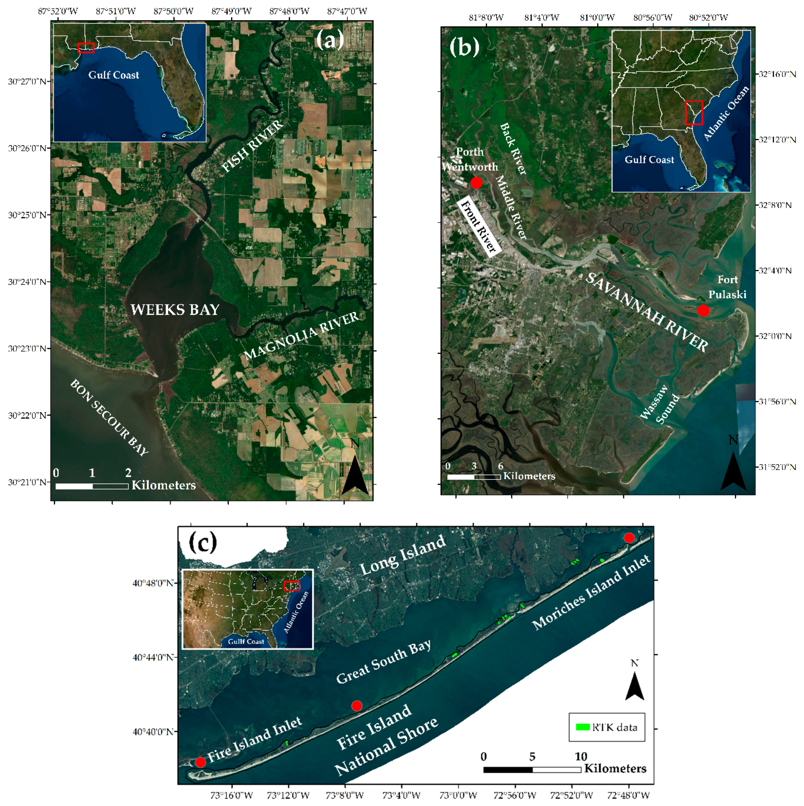
2.1. Study Area

We selected two estuarine systems and one barrier island for this study: Weeks Bay, located on the Gulf of Mexico Coast of the United States, and Savannah Estuary and Fire Island, located on the Atlantic Coast of the United States. We studied these two estuaries with different hydro-morphological characteristics such as size, mean depth, riverine to tidal influence, anthropogenic interventions and ecological characteristics to assess the broader applicability of our proposed methodology in different estuarine systems. In addition, we extended our analysis on Fire Island to validate our results with publicly available RTK topographic survey data.

Weeks Bay is a shallow, diamond shaped, microtidal estuary located along the eastern shore of Mobile Bay in Baldwin County, Alabama (Figure 1a). Weeks Bay is a tributary estuary of Mobile Bay and has been designated as a National Estuarine Research Reserve (NERR) site since 1986 [37]. The estuary has a surface area of approximately 7 km² with a longitudinal axis (north to south) of 3.4 km and a transversal axis (west to east) of 3.1 km [38]. Freshwater discharge into the estuary comes from the Fish River and Magnolia River located at the northern and eastern sides of the Bay, respectively. Fish River provides ~73% of total freshwater input (~ 9 m³/s), while Magnolia River supplies the rest. Mean depth of Weeks Bay is about 1.5 m, with maximum local depths up to 7 m (see the deep area connecting Bon Secour Bay to Weeks Bay for example) [39]. The tidal regime is predominantly diurnal with tidal range of 0.4 m and currents exceeding 1 m/s at the mouth of the bay [40]. The estuarine system consists of deepwater tidal habitats and adjacent tidal wetlands which are regularly flooded by tides [18].

Savannah River originates at the confluence of the Tulagoo and Seneca Rivers at Hartwell, Georgia and debouches into the Atlantic Ocean (Figure 1b). The river flows in a southeastern direction and serves as a ~500 km natural border of South Carolina and Georgia. Savannah River estuary extents from Port Wentworth to Fort Pulaski (at the estuary mouth) and comprises the lower ~50 km of the river [41]. The river channel from Port Wentworth to Tybee Range has been deepened for navigation purposes with a mean depth of 12 m below mean low water as reported by the U.S. Army Corps of Engineers [42]. Furthermore, the U.S. Army Corps of Engineers constructed three major dams (J. Strom Thurmond, Richard B. Russell, and Hartwell) on the Savannah River, mainly for hydroelectric generation, flood control and water supply management purposes [43]. Savannah River at Port Wentworth trifurcates in distributary channels named Front, Middle and Back rivers as (Figure 1b). The annual averaged discharge to the estuary and tidal range at the estuary mouth are approximately 359 m³/s and 2.5 m, respectively [41]. The estuarine system consists of deepwater tidal habitats and adjacent tidal wetlands which are regularly flooded by tides, and partly drained wetlands that have been altered hydrologically. Anthropogenic intervention is also evident in wetlands containing and connected to ditches [18].

Fire Island, a 50-km-long barrier island with varying width from 200 m to 1 km [44], is located at the south shore of Long Island in Suffolk County, New York (Figure 1c). The island holds a variety of salt marsh species and vegetation distributed along the barrier. Fire Island is currently constrained by two main tidal inlets used as navigation channels: Fire Island Inlet to the west and Moriches Inlet to the east. The barrier island has been affected by extreme storm surges, such as Hurricane Sandy in 2012 which caused overwash on 41% of Fire Island and modified its shape due to large amount of sediment accumulation (approximately 50,800 m³) [20]. From fall 2014 to spring 2016, an extensive RTK topographic survey over salt marsh regions was conducted on Fire Island as described in Section 2.2. These data are further used in Section 3.4 for validation of the proposed tool.

2.2. Data

We used imagery datasets (i.e., band collection) from both Landsat 8 OLI/TIRS (Collection 1 Level-1) and Landsat Analysis Ready Data (ARD) archives since the application of the former in land cover classification is affected by atmospheric errors [21]. Contrary to Landsat 8 OLI/TIRS, Landsat ARD is a surface reflectance product [45] with imagery corrected for atmospheric attenuation (e.g., scattering and absorption effects). However, Landsat ARD does not contain the thermal and panchromatic bands as they are not surface reflectance products. We used the panchromatic bands of Landsat 8 OLI/TIRS to enhance the spatial resolution of the images in OBIA and RF as further described in Section 2.4. Both datasets, covering the hydrologic catchments of the study areas in 2016 and 2019, are open source and can be obtained from the Earth Explorer website (https://earthexplorer.usgs.gov). In addition to the imagery datasets, we used the geo-database of the NWI (https://fwsprimary.wim.usgs.gov/wetlands/apps/wetlands-mapper/) and the ‘C-CAP 2010-Era Land Cover’ map (https://coast.noaa.gov/digitalcoast/tools/lca.html) of the National Oceanic and Atmospheric Administration (NOAA) and the National Ocean Service (NOS) as references to discriminate emergent wetlands in the study area.

We obtained LiDAR-derived DEMs of Weeks Bay (i.e., 2014 Northern Gulf of Mexico dataset), Savannah Estuary (i.e., 2017 Coastal South Carolina dataset), and Fire Island (i.e., 2017 East Coast dataset) from NOAA’s Data Access Viewer (https://coast.noaa.gov/dataviewer/#). The DEMs have horizontal datum: UTM Zone 16N, 17N and 18N—North American Datum 1983 projection (NAD83); North American Vertical Datum 1988: NAVD88; and spatial resolution: ~3 × 3 m (1/9th arc-second), 1 × 1 m and 1 × 1 m, respectively. We also obtained information about the mean high water (MHW), mean sea level (MSL) and mean low water (MLW) datum referenced to NAVD88 for surface elevation correction (described in Section 2.5) from NOAA (https://tidesandcurrents.noaa.gov).

For validation of the DEM-correction tool, we used a set of 1530 RTK points (i.e., ground-truth marsh elevation) collected by staff of the Environmental Data Center (EDC) in cooperation with the Northeast Coastal and Barrier Network (NCBN) at strategic marsh locations in Fire Island (Figure 1c). This dataset is publicly available and can be obtained from the Integrated Resource Management Applications (IRMA) database (https://irma.nps.gov/DataStore/Reference/Profile/2240329). The RTK data has a spatial resolution of 20 m referenced with respect to horizontal datum: UTM Zone 18N—NAD83 (2011) and vertical datum: NAVD88.

2.3. Imagery Preprocessing

We selected the time frame of single images in this study based on two conditions: (1) consistency with Landsat imagery used in the 2016 NLCD for land cover classification over the study areas; and (2) imagery preferably captured within MLW in order to avoid tidal inundation effects land cover classification [46,47]. In addition, we obtained Landsat 8 OLI/TIRS and ARD images from Earth Explorer applying a cloud cover filter less than 20% in order to be consistent with the proposed steps for land cover classification of the 2016 NLCD [17]. We further preprocessed some images with the fmask tool [48] to get rid of clouds and shadows in our analyses. A summary of the imagery datasets used in this study including tidal stage during image acquisition is presented in

Table 1. Imagery dataset used in land cover classification of the 2016 National Land Cover Database (NLCD) (reference) and the dataset used for image segmentation, feature extraction, training and validation, and updating emergent herbaceous wetland regions.

NLCD (Reference)	Date	Landsat 8 OLI/TIRS § (Path/Row)	Landsat ARD # (Horiz./Vert.)	Tidal Stage * (Max/Min/Mean) (m)	Study Area
2016/Mar/03	2016/Feb/28	20/39	22/16	0.14/–0.14/0.00	Weeks Bay
N/A	2019/Apr/16			0.21/–0.12/0.04
2016/May/17	2016/May/06	16/38	26/14	1.73/–1.48/0.19	Savannah
N/A	2019/Apr/29			0.86/–0.87/0.05
2016/Jun/17	2016/Jun/18	13/32	29/7	0.24/–0.19/0.02	Fire Island
N/A	2016/Apr/24			0.42/–0.09/0.16

^§ Operational Land Imager/Thermal Infrared Sensor; ^# Analysis Ready Data; * Referenced with respect to NAVD88.

. The selected tidal gauges for Weeks Bay, Savannah Estuary and Fire Island were Dauphin Island, Alabama (NOAA station 8735180), Fort Pulaski, Georgia (NOAA station 8670870) and Great South Bay at Watch Hill, New York (USGS station 01305575), respectively.

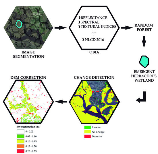
2.4. Updating Emergent Wetland Regions

The updating process of emergent wetland regions to present-day (2019) conditions involved three steps: (1) image segmentation with OBIA; (2) feature and land cover class extraction; and (3) training and validation with RF technique.

2.4.1. Image Segmentation with OBIA

To conduct the image segmentation, we first masked the clouds and shadows in the study area with the fmask tool [48] and then pansharpened the Landsat 8 OLI/TIRS imagery datasets (Table 1) with the Gram–Schmidt method (ArcGIS 10.6.1) as suggested in similar studies [19,49]. The pansharpening process leverages the high spatial resolution of the panchromatic band (15 m) and replaces its low spectral resolution with the high spectral resolution of the other bands in the band collection. The multispectral bands used in this process (with equal band weight) were B5 (near-infrared); B3 (green); B2 (blue); B8 (panchromatic). It is important to note that B5 was preferred over B4 (red) since the near-infrared band can better distinguish differences in spectral signatures from vegetated and non-vegetated areas [21,50]. The resulting multispectral images therefore have high spatial and spectral resolution, and also highlight vegetated areas of the study area. We then used OBIA to divide the multispectral images into heterogeneous polygons (or objects) comprising areas with similar spectral properties. The objects were generated through the ‘Mean-Shift’ segmentation algorithm included in the Orfeo Toolbox (OTB 6.6.0) [51], and available in QGIS as an external plugin. This method has been used in other studies with satisfactory results [20,52,53]. It is worth mentioning that the polygon heterogeneity (i.e., size of the objects) is controlled by user-defined parameters. The main parameters used in this study and their corresponding values are spatial radius (5), range/spectral radius (10), and minimum region size (15). The remaining parameters were set to default values. The optimal (main) parameter-values were found empirically by testing different sets of values systematically (e.g., ranging from 5 to 40) [23]. This process was repeated until emergent wetland regions were properly delineated and/or separated from open water. Furthermore, the resulting polygons were visually compared to reference land cover maps (e.g., C-CAP and NWI).

2.4.2. Feature and Land Cover Class Extraction

At this stage we computed and extracted features and land cover classes to build a learning database for the RF algorithm. Since the Landsat 8 OLI/TIRS imagery is affected by atmospheric attenuation [21,45], we conducted feature extraction from ARD imagery that is a surface reflectance product (Table 1). We classified the computed features in three groups: reflectance, spectral and textural indices [19,21]. The reflectance features, characterized via mean, standard deviation and range, were obtained from two multispectral band compositions: B4 (red); B3 (green); B2 (blue) and B5 (near-infrared); B3; B2. The spectral and textural indices from vegetated and non-vegetated areas are characterized via mean and standard deviation (SD) as indicated in

Table 2. Feature extraction from Landsat Analysis Ready Data (ARD) imagery based on reflectance, spectral and textural indices.

Features	Variables (p)	Expression
Reflectance (mean, SD, and range)	Multispectral band composition	Red; Green; Blue
		NIR|; Green; Blue
Spectral indices (mean and SD)	Normalized Difference Vegetation Index (NDVI)	$\frac{NIR-Red}{NIR+Red}$
	Normalized Difference Water Index (NDWI)	$\frac{Green-NIR}{Green+NIR}$
	Brightness Index (BI)	$\sqrt{Re{d}^2+Gree{n}^2+Blu{e}^2+NI{R}^2}$
	Enhanced Vegetation Index (EVI)	$2.5\ast \frac{\left(NIR-Red\right)}{NIR+6\ast Red-7.5\ast Blue+1}$
	Normalized Difference Built-up Index (NDBI)	$\frac{SWI{R}^{\nparallel }-NIR}{SWIR+NIR}$
	Specific Leaf Area Vegetation Index (SLAVI)	$\frac{NIR}{Red+NIR}$
	Green Ratio Vegetation Index (GRVI)	$\frac{NIR}{Green}$
	Ratio Vegetation Index (RVI)	$\frac{Red}{NIR}$
Textural indices (mean and SD)	Contrast	Focal Statistics
	Entropy	Haralick Texture
	Haralick correlation

^| Near-infrared; ^∦ SWIR: Short-wave infrared.

. Moreover, the number of variables ‘p’ is 28 as presented in the same table. The textural indices were computed with both the ‘Haralick Texture’ features of OTB in QGIs and ‘Focal Statistics’ in ArcGIS; and based on window sizes of 5 × 5 pixels with band composition of B5; B3; B2; B. B5 was preferred over B4 as the near-infrared band might contrast better soil-vegetation discontinuities than the red band [19]. Haralick texture is a widely used parameter for texture recognition as it measures consistency of patterns and colors in image objects [54]. Focal statistics computes a set of statistics (e.g., mean, standard deviation, range) based on information of neighbor raster cells, and hence identifies image objects sharing similar properties (e.g., reflectance, spectral and textural). Lastly, we extracted the land cover classes of Weeks Bay and Savannah Estuary from the 2016 NLCD to further train and validate the RF algorithm as described in the next section.

2.4.3. Training and Validation with Random Forest

In this stage, we trained and validated the RF learning algorithm in Python 3.7 with the features extracted from the 2016 imagery and the land cover classes of the 2016 NLCD. This process requires three steps: (i) assembling the learning database; (ii) establishing a hierarchical approach for land cover classification; and (iii) hyperparameter tuning of the random forest algorithm including accuracy assessment. The ultimate goal of this stage was to classify and update emergent wetland regions in the 2019 imagery as described in Section 3.3.

• Assembling the learning database

We used ArcGIS to join and relate all the features and land cover classes extracted in the second stage to the polygons (or objects) generated through image segmentation in the first stage. Hence, each polygon feature (identified with a unique ID) displays a set of reflectance, spectral and textural indices that belongs to a specific land cover class. Since the numbers of objects generated in Weeks Bay and Savannah Estuary are relatively large (i.e., 102,983 and 105,580, respectively), we trained and validated the RF with a random sample consisting of 25% of all the polygon features per study area in order to reduce computation effort while also ensuring model robustness. Moreover, large training sample sizes could affect the proportion between land cover classes, and thus decreasing the overall accuracy of the RF algorithm [55]. The total number of objects generated in Fire Island, on the other hand, was approximately 5% of those of Weeks Bay or Savannah Estuary (i.e., 5026). This in turn suggests that the random sample could be increased as there is always a trade-off between high accuracy (model robustness) and computation time. We therefore used a random sample consisting of 50% of all polygon features for Fire Island. Furthermore, we dealt with unbalanced data in the sampling process by computing the class weight of each land cover class and using a fixed seed value (i.e., random state = 0) for reproducibility. The sample data therefore had a balanced number of polygons per land cover class. Likewise, we divided the sample data into two parts for training (70%) and validation (30%) with the fixed seed value to ensure reproducibility.

• Hierarchical approach for land cover classification

We followed a hierarchical approach to discriminate land cover classes from each other. Contrary to the classical approach, in which the entire learning database is used to generate RF classifiers at each nomenclature level, the hierarchical approach separates the database according to user-defined levels and then generates classifiers for each nomenclature level. Moreover, this approach significantly improves land cover classification accuracy at all nomenclature levels, compared with the classical approach as reported in Lebourgeois et al. [19]. In this study, we arranged the polygon features (and associated indices) into three levels based on the 2016 NLCD classification: (L1) urban and non-urban areas, (L2) vegetated and non-vegetated areas and (L3) wetland areas, as indicated in

Table 3. Nomenclature levels and number of polygon features (Weeks Bay/Savannah/Fire Island) used to validate the random forest classifiers for land cover classification.

Level 1 (L1)	Level 2 (L2)	Level 3 (L3)
Urban areas (1979/2097/135)	Developed, open space (797/736/21)	NA
	Developed, low intensity (650/667/69)
	Developed, medium intensity (444/417/36)
	Developed, high intensity (88/277/9)
Non-urban areas (5639/5607/599)	Open water (504/873/203)	NA
	Deciduous, Evergreen and Mixed forest (1028/1117/23)
	Barren land, Grassland, Herbaceous, Pasture and Shrub (1887/1332/203)
	Cultivated crops (882/516/NA)
	Wetlands (1338/1769/170)	Woody (845/902/14)
		Emergent herbaceous (493/867/156)

. The number of polygons per level and study area is mentioned between parentheses below each land cover class.

• Hyperparameter tuning of random forest and accuracy assessment

The next step was to find optimal hyperparameter values to build the decision tree classifiers in the RF algorithm. We used the scikit-learn tool package of Python to conduct a ‘Hyperparameter Tuning’, and hence account for overfitting through cross-validation (CV) [56]. For the hyperparameter tuning, we first created a grid with empirical range-values based on recent studies [55,57,58,59,60]. We randomly generated the hyperparameter values within the established ranges, avoiding a fixed interval between two consecutive values as indicated in

Table 4. Hyperparameter grid used for a 5-fold cross-validation.

Hyperparameter	Range	Total
Number of estimators	100–600	5
Maximum features	10–20	5 †
Maximum depth	30–50	4
Minimum sample split	2–6	3
Minimum sample leafs	3–7	3
Bootstrap	True or False	2

^† Including ‘sqrt’ and ‘none’.

. In addition, we use a ‘stratified k-fold’ approach to divide the data into training and testing sets in the CV process. The number of k-folds is set to 5 as suggested in similar studies [19,61,62] and the grid is generated with the fixed seed value for reproducibility. We then used the grid in the ‘Randomized Search CV’ function to randomly sample a set of hyperparameter values and conduct a stratified k-fold CV with each combination of values. The number of combinations to be tested in the function is defined by the ‘n_iter’ parameter which in our study was set to 100. As a result, the total number of fits, defined as k-folds × n_iter, led to 500 CV computations.

To determine the best combination of values, each single combination was evaluated recursively in the validation dataset (i.e., 30% of the sampling data) by generating a confusion matrix and calculating three metrics related to land cover classification: overall accuracy, f1-score (per class and macro), and Kappa coefficient. These metrics have been widely used to assess land cover classification in multiple studies [19,20,21,43,55,58]. Hence, we quantitatively assessed actual vs. computed land cover class of each polygon (or object). Lastly, we defined the optimal hyperparameter values of each study area by refining our search around the best combination of values determined with the previous function. We use the ‘Grid Search CV’ function to evaluate specific user-defined combinations of values and obtain the highest metrics per study area. The optimal hyperparameter values and the corresponding accuracy assessment indices are presented in Section 3.1 and Section 3.2, respectively.

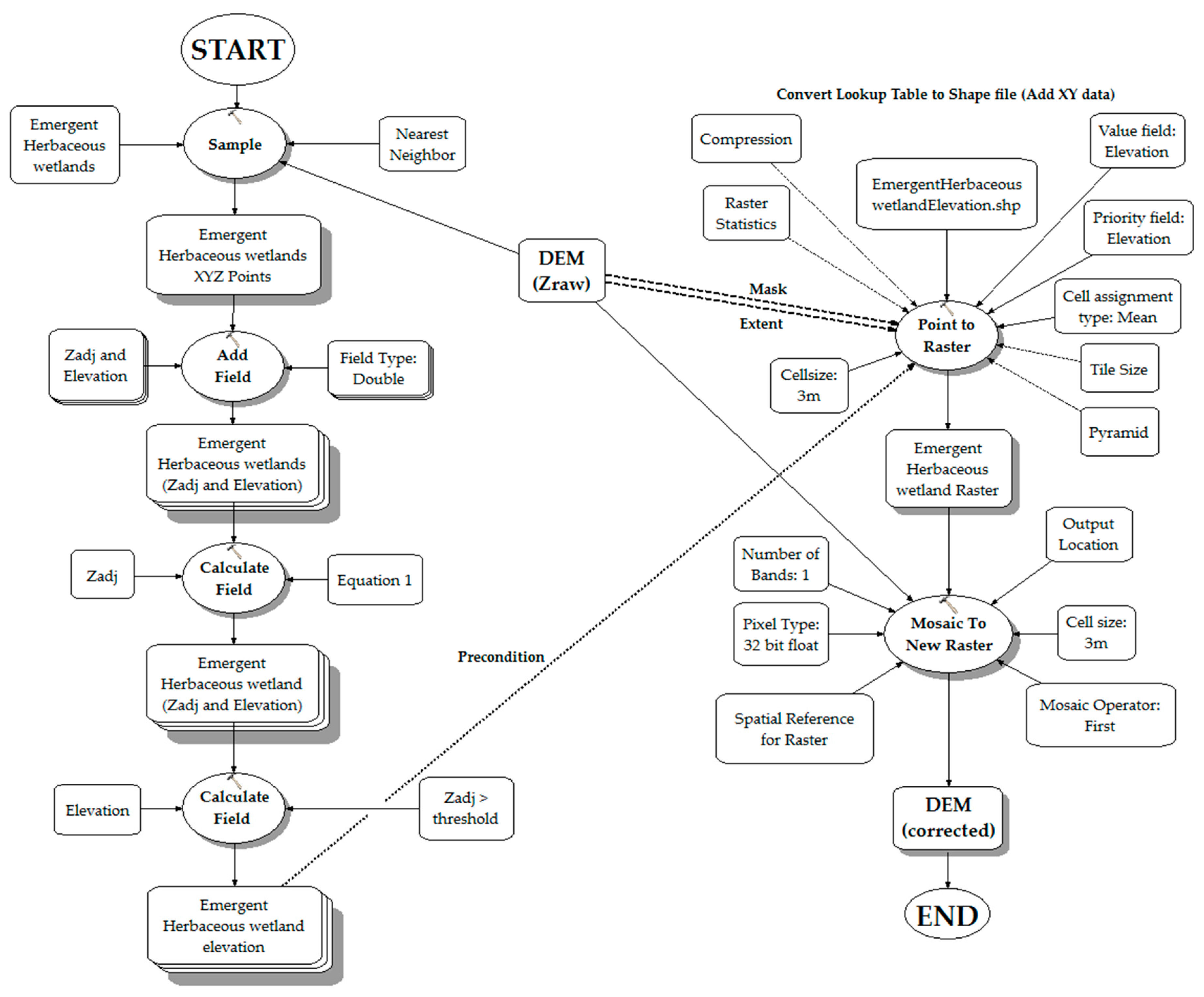
2.5. Adjusting Emergent Wetland Surface Elevation

Emergent wetlands growing in estuarine systems of the Atlantic and Gulf Coasts of the U.S. consist of different vegetation species, but salt marshes in particular lead to the highest LiDAR elevation errors [6,35]. Therefore, we selected those regions for further elevation adjustment and DEM correction. Alizad et al. [8] corrected salt marsh elevation in Grand Bay and Weeks Bay in terms of marsh productivity and above-ground biomass density of vegetation species from Apalachicola Bay. The authors pointed out that marsh productive areas in the Apalachicola Bay are located in the upper portion of the tidal frame, and hence this elevation can be used to guide the salt marsh platform adjustment in the other two bays. Furthermore, they proposed the following equation to vertically position salt marsh platforms relative to the tidal frame similar to Apalachicola Bay:

$$z_{adj}=\frac{\left(u-l\right)\left(z_{raw}-z_{min}\right)}{z_{max}-z_{min}}+l$$

(1)

where z_adj is the adjusted elevation; u and l are the desired upper and lower limits of the adjusted elevation, respectively; and z_max and z_min are the actual maximum and minimum raw elevations (z_raw) of the DEM cell to be adjusted in the domain. It is important to note that elevations lower than (or equal to) a threshold value (i.e., lower limit) should not be adjusted as this would unnecessarily flatten the micro-topography of small tidal creeks, and consequently alter the inundation patterns [8].

To apply Equation (1) in Weeks Bay and Savannah Estuary, we referenced MHW, MSL and MLW with respect to the vertical datum NAVD88 of Dauphin Island and Fort Pulaski, respectively (Table 1). Although Fire Island has its own representative tidal gauge (i.e., USGS station 01305575), this station has been recording water heights since mid-April 2016 to present. As a result, the present National Tidal Datum Epoch (i.e., from 1983 up to 2001) used to calculate MHW, MSL and MLW is outside the time-frame of available water height records. We therefore estimated these datum data from a nearby tidal gauge station with longer records located at Montauk, New York (NOAA station 8510560). The upper tide range was calculated by subtracting MSL from MHW, and the upper midpoint of the tidal frame (lower limit) by adding half of the upper tide range to the MSL. Also, the upper limit was calculated by adding the upper tide range to the MHW, and z_max obtained from a frequency analysis of salt marsh elevation in the unadjusted DEM. A summary of these variables is presented in

Table 5. Tidal datum and variables of Equation (1) used for salt marsh elevation correction.

Variable [m]	Dauphin Island, AL (8735180)	Fort Pulaski, GA (8670870)	Fire Island, NY (8510560)
Mean high water (MHW)	0.207	0.938	0.205
Mean sea level (MSL)	0.018	−0.071	−0.101
Mean lower water (MLW)	−0.151	−1.170	−0.426
Upper tide range	0.189	1.009	0.306
Upper midpoint	0.113	0.434	0.052
Upper limit (u)	0.396	1.947	0.511
Lower limit (l)	0.113	0.434	0.052
zmax	1.150	1.950	1.035
zmin	0.113	0.434	0.052

.

Implementation of the DEM-Correction Tool

We used Table 5 and Equation (1) to implement a tool aimed at automating salt marsh elevation correction. Since Equation (1) is based on salt marsh productivity and above-ground biomass density of biologically similar species, we assume the equation does not alter the natural elevation of other vegetated species contained in the emergent herbaceous wetland class. The implementation of the DEM-correction tools is described as follows.

First, the tool extracts the ground-surface elevation points of emergent herbaceous wetlands from the DEM (i.e., z_raw) with a nearest neighbor resampling technique. We used the ‘Sample’ tool to create a temporary lookup table containing the raster cell-values from those regions (i.e., X, Y and Z-coordinates). Subsequently, we extract the maximum and minimum elevations (i.e., z_max and z_min) of the emergent wetland regions from the lookup table. The second and third steps are to calculate the adjusted elevation (i.e., z_adj) as indicated in Equation (1) and compare this value to the threshold value (i.e., lower limit). The resulting ‘Emergent Herbaceous wetland elevation’ dataset is then manually transformed into point features through the ‘Add XY data’ option in ArcGIS and stored in a shape file format for further use. The fourth step is to convert the point features in raster cell-values through the ‘Point to Raster’ tool. We set the cell size, cell assignment type and value/priority field to 3 m, mean value and ‘Elevation’, respectively. The remaining parameters of the tool were set to default. The final step is to combine the resulting ‘Emergent Herbaceous wetland Raster’ dataset with the DEM input of Weeks Bay or Savannah Estuary. We use the tool ‘Mosaic to New Raster’ to merge the two raster datasets by prioritizing the adjusted raster cell-values of the salt marsh regions with the ‘Mosaic Operator’ parameter. Finally, we set the cell size, pixel type, and number of bands to 3 m, 32-bit float and single band, respectively. Figure 2 presents a workflow of the DEM-correction tool created in Model Builder of ArcGIS. The results of the surface elevation correction in Weeks Bay and Savannah Estuary are presented in Section 3.4.

3. Results

3.1. Optimal Hyperparameter Values

We conducted hyperparameter tuning in the two estuaries separately. The optimal values at each nomenclature level were almost identical with slight variations (i.e., order of units) mainly in the number of estimators and maximum features. For that reason, we used the same optimal values at each nomenclature level for further computations.

Table 6. Optimal hyperparameters used for land cover classification at each nomenclature level.

Hyperparameter	Weeks Bay	Savannah	Fire Island
Number of estimators	500	550	563
Maximum features	18	16	16
Maximum depth	37	37	49
Minimum sample split	4	4	4
Minimum sample leafs	5	3	3
Bootstrap	True	True	True

presents the optimal values per study area. In general, the optimal hyperparameter values were not far from each other when comparing the two estuaries. The largest difference was observed in the number of estimators, which was greater by 50 units in Savannah Estuary.

3.2. Accuracy Assessment of Land Cover Classification

We quantitatively assessed the accuracy of land cover classification at each nomenclature level in terms of overall accuracy, f1-score (class and macro) and Kappa coefficient as presented in

Table 7. Accuracy assessment of land cover classification (Weeks Bay/Savannah/Fire Island) during training and validation of the random forest algorithm.

Nomenclature Level	Description/Land Cover Class	Overall Accuracy	Class f1-score	f1-score Macro	Kappa Coefficient
L1	Urban areas	(0.86/0.90/0.86)	(0.71/0.81/0.60)	(0.81/0.87/0.76)	(0.62/0.74/0.51)
	Non-urban areas		(0.90/0.93/0.92)
L2	Developed, open space	(0.65/0.73/0.70)	(0.76/0.83/0.65)	(0.63/0.73/0.68)	(0.49/0.63/0.54)
	Developed, low intensity		(0.55/0.66/0.72)
	Developed, medium intensity		(0.62/0.63/0.71)
	Developed, high intensity		(0.59/0.82/0.67)
	Open water	(0.73/0.75/0.87)	(0.93/0.96/0.95)	(0.75/0.73/0.76)	(0.65/0.67/0.82)
	Deciduous, Evergreen and Mixed forest		(0.64/0.65/0.37)
	Barren land, Grassland, Herbaceous, Pasture and Shrub		(0.74/0.70/0.88)
	Cultivated crops		(0.72/0.56/NA)
	Wetlands		(0.72/0.80/0.83)
L3	Woody	(0.91/0.97/0.95)	(0.93/0.97/0.69)	(0.90/0.97/0.83)	(0.80/0.95/0.66)
	Emergent herbaceous		(0.88/0.97/0.97)

. At the first level (L1), the RF was able to discriminate urban from non-urban areas with moderate-high to high accuracies regarding the three metrics. Nevertheless, the Kappa coefficient was relatively low in Weeks Bay with a value of 0.62. At the second level (L2), the RF algorithm discriminated the land cover classes within the two groups of L1. When comparing the metrics of developed areas to undeveloped areas (i.e., open water, forests, crops, wetlands, etc.), we observe that RF was slightly better in identifying vegetated areas than developed areas. This might be related to the large extent of shrubs and wetlands around the estuaries, even though we dealt with unbalanced classes when sampling the data (see Section 2.4.3 for details). Moreover, the latter may have led the RF to learn more about the properties of those land covers compared to developed areas. As a result, the highest class f1-score belonged to shrubs in Weeks Bay (0.74) and wetlands in Savannah Estuary (0.80). At the third level (L3), the metrics suggested that RF algorithm was able to identify emergent herbaceous wetlands with high accuracies (up to 0.97). As expected, better results were derived from Savannah Estuary due to its larger wetland areas.

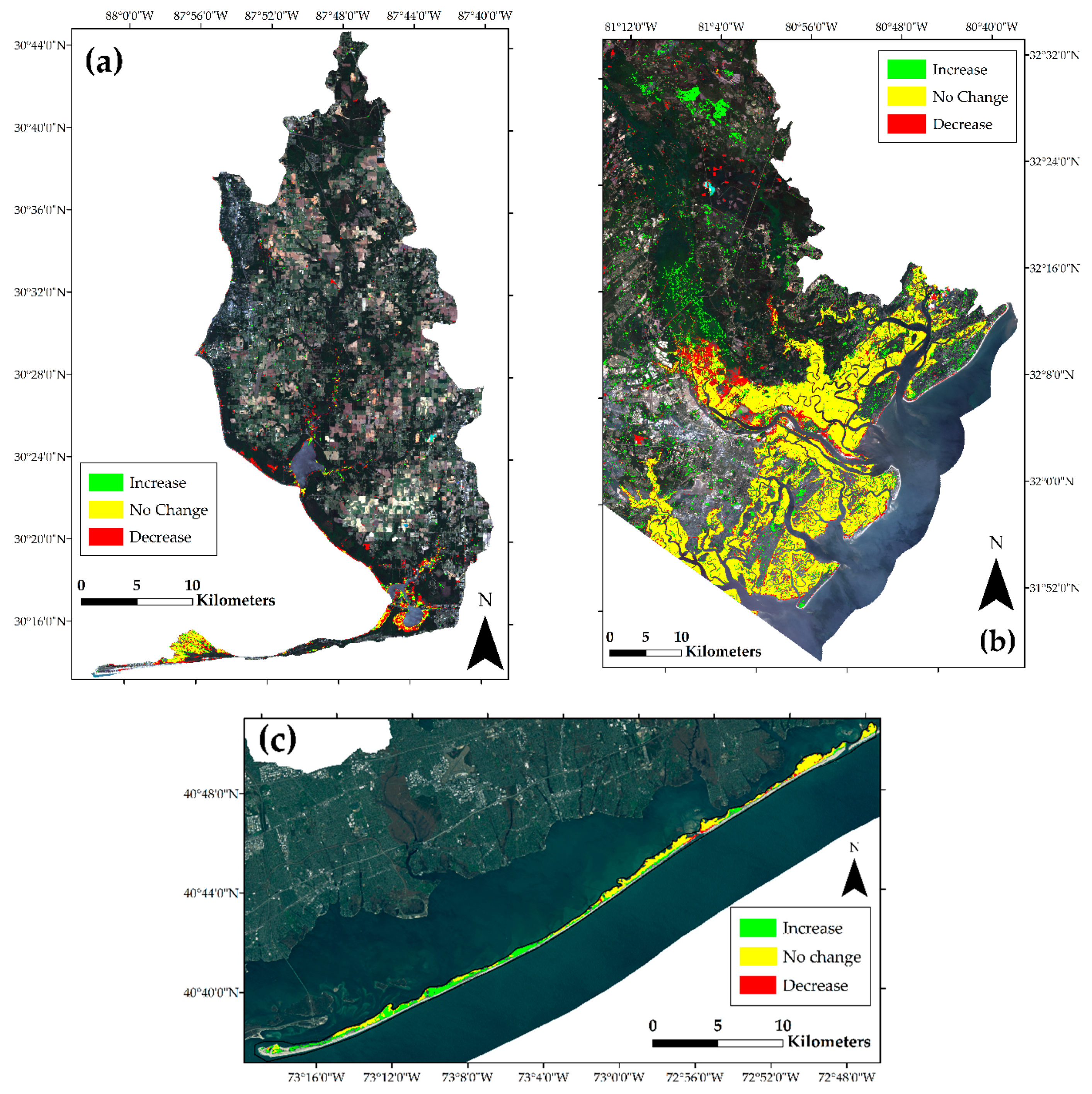
3.3. Emergent Wetland Classification in the 2019 Imagery

We conducted a land cover classification using the polygons created in the 2019 imagery with the associated indices (see Section 2.4 for details) and the optimal hyperparameters of each study area (Table 6). Then, we grouped the emergent herbaceous wetland class to further correct salt marsh elevation as described in the next subsection. Figure 3 shows land cover change detection within emergent wetland areas obtained with OBIA and RF. Note that Savannah Estuary exhibits a larger wetland area than Weeks Bay as discussed in the previous subsection.

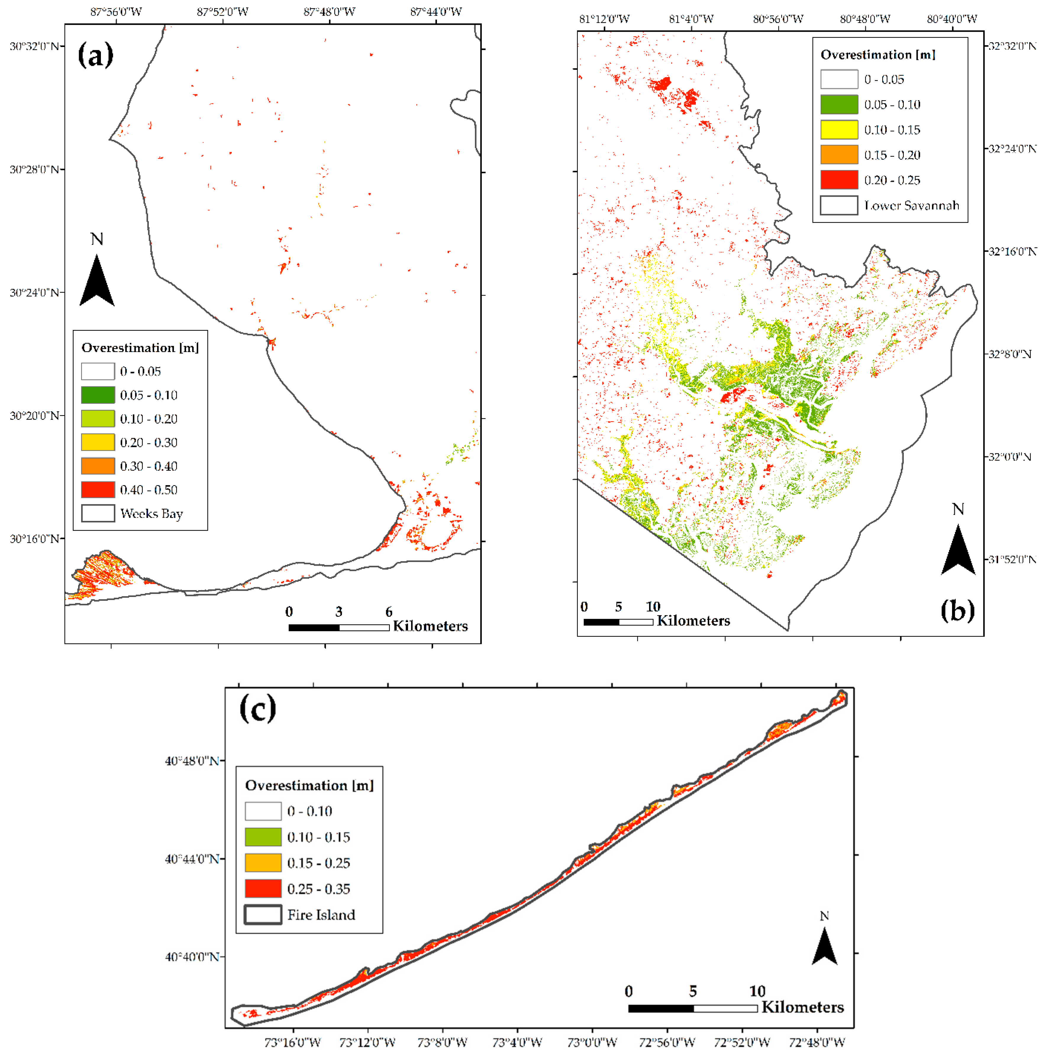
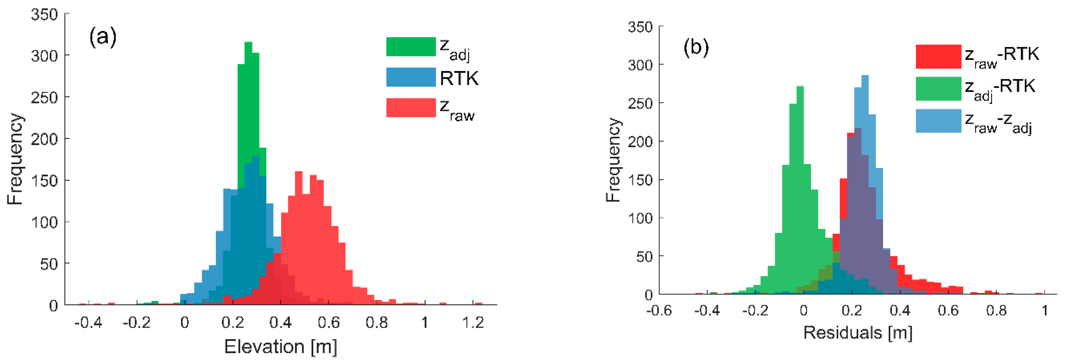
3.4. Adjusting Emergent Wetland Surface Elevation in DEMs

We used the DEM-correction tool to adjust marsh elevation and generate a modified DEM. In order to compare the existing and modified DEM, we computed the overestimation in surface elevation over marsh regions as presented in Figure 4. The largest overestimation was observed in Weeks Bay with maximum values of 0.50 m followed by Fire Island and Savannah Estuary with 0.35 and 0.25 m, respectively. After surface elevation correction, no manual adjustment was conducted to ensure a proper evaluation of the proposed tool as described in the next section.

DEM-Correction Accuracy Assessment

We evaluated the performance of the DEM-correction tool by conducting statistical analyses of ground-truth marsh elevation points (i.e., RTK) of Fire Island (Figure 1c). Likewise, we used the spatial (x-y) coordinates of each point to extract the overlying elevation of the adjusted (z_adj) and unadjusted (z_raw) DEM. We then compared these elevations under the assumption that the entire emergent herbaceous wetland class follows a normal distribution as indicated in Figure 5a. We also conducted an analysis of frequency of errors (i.e., residuals) to evaluate the performance of the DEM-correction tool in mean error reduction (Figure 5b). For convenience, we also calculated the residual between z_adj and RTK.

Table 8. Summary of residual analysis (vertical error) within emergent herbaceous wetlands of Fire Island, New York.

Residuals	Max. (m)	Min. (m)	Range (m)	ME (m)	SE (m)	RMSE (m)
zraw - RTK	1.319	−0.926	2.245	0.250	0.004	0.008
zadj - RTK	0.624	−0.481	1.105	0.003	0.003	0.003
zraw - zadj	1.310	−0.451	1.761	0.247	0.003	0.007

summarizes the results of this analysis in terms of mean error or overall bias (ME), standard error (SD) and root-mean-square error (RMSE).

4. Discussion

Although several studies have used default parameter values (or recommended values) in RF with satisfactory results [21,43,63,64], tuned parameter values can improve the performance of RF and thus lead to high accuracy in land cover classification [55,60]. In this study, we followed a hyperparameter tuning approach with stratified 5-fold cross-validation for Weeks Bay, Savannah Estuary and Fire Island, separately. As reported in similar studies [19,26,43], the recommended number of trees is 500 and the maximum number of features is given by p^1/2 (e.g., we set p = 28 and/or p^1/2 ~ 5 as indicated in Section 2.4.2). The last parameter value differs moderately (order of tens) with respect to the optimal values we presented in Table 6 even though the number of trees is close to the values reported in this study. In addition, we observed slight variations of optimal values (order of units) at each nomenclature level and study area, and for that reason, we used constant optimal values in further computations (Table 6). Nonetheless, the results with constant optimal values led to land cover classification with moderate to high accuracies at each nomenclature level (Table 7).

Since this study is focused on updating emergent wetlands, we trained the RF with a third nomenclature level which in turn produced the highest accuracies in Weeks Bay, Savannah Estuary and Fire Island regarding the f1-scores (0.88, 0.97, 0.97), Kappa coefficient (0.80, 0.95, 0.66) and overall accuracy (0.91, 0.97, 0.95) in the 2016 imagery dataset. We ultimately used the optimal parameter values to discriminate emergent herbaceous wetlands (among other land cover classes) in the 2019 imagery dataset since the NLCD is infrequently updated. Hence, using an updated wetland class is of value as for further analysis such as salt marsh migration patterns due to sea level rise and coastal erosion. Figure 3 highlights wetland areas in the two estuaries and barrier island which have been visually validated with 2019 Landsat imagery. The validation suggests that developed (urban) zones (e.g., <1800 m² or 3 pixel units) surrounded by larger emergent herbaceous wetland areas (e.g., Savannah Estuary and Fire Island) are often misclassified mainly due to the moderate resolution of Landsat imagery, which is not able to accurately discriminate these two areas even with pansharpened images. Misclassification errors could be overcome by either using available high or ultra-high resolution imagery as indicated in similar studies [20,23,65,66] as well as reducing the size of objects in the image segmentation process. Even though smaller objects can better delineate urban features (e.g., streets, parking lots, squares), they might also increase computation effort when integrating OBIA and RF in large catchment areas (e.g., Lower Savannah, Figure 3b).

We evaluated salt marsh elevation correction comparing the difference in elevation within corrected (modified) and original DEMs (Figure 4). Even though salt marsh areas in Savannah Estuary and Fire Island are larger than Weeks Bay, we obtained the largest overestimation in elevation (up to 0.50 m) in Weeks Bay, probably due to different LiDAR-derived DEM inputs for each estuary. As described in Section 2.2, the most updated DEM of Weeks Bay, Savannah Estuary and Fire Island correspond to 2014, 2017 and 2017, respectively. Therefore, Weeks Bay is likely to present relatively larger vertical errors, compared to the other study areas, due to salt marsh migration and/or land cover change effects. Savannah, on the other hand, presented overestimation in salt marsh elevation up to 0.25 m particularly in upstream areas of the Savannah River. When visually verifying the land cover classification, we identified a misclassified area at the upper left zone of Figure 3. This ‘Mixed and Evergreen Forest’ area located far away from the estuary was erroneously classified as emergent herbaceous wetland, which in turn led to high vertical errors (0.25 m) as shown Figure 4. Likewise, Fire Island showed maximum overestimation (up to 0.35 m) in marsh region along the barrier island. In contrast to the two estuarine systems, Fire Island has publicly available RTK data which in turn served to validate the performance of the DEM-correction tool.

Figure 5a indicates that the mean elevation of z_raw (~0.50 m) clearly overestimates the true mean RTK elevation (~0.25 m) by a factor of two. However, after linear adjustment through Equation (1), the adjusted mean elevation (~0.26 m) is almost identical to the ground-truth mean elevation. Nevertheless, it is worth noting that Equation (1) also modifies the natural spread of marsh elevation by narrowing its standard deviation. Likewise, extreme maximum and minimum values presented in Figure 5 and Table 8 might be outliers due to errors in RTK data collection and/or LiDAR sensors commonly used for DEM generation. In addition, Figure 5b and Table 8 suggest that the DEM-correction tool can effectively lead to identical ME, SE and RMSE when adjusting z_raw with respect to RTK elevation data. Furthermore, we calculated the vertical error between z_adj and RTK and observed that ME, SE and RMSE are in the order of mm. The latter suggests that the proposed tool can confidently be used for rapid and reliable assessment of LiDAR elevation error in coastal wetlands without any species-level classification. Although other studies suggest that distribution of vegetation height shows unique characteristics depending on the species analyzed [6,35], we assumed that RTK elevation data may follow a normal distribution provided that the entire emergent herbaceous wetland class is used in absence of accurate species-level classification (Figure 5). We therefore propose a methodology for elevation adjustment in wetlands that can easily be followed with readily available data (i.e., Landsat imagery of moderate resolution and DEMs) and high accuracy.

5. Conclusions

Adequate representation of salt marsh elevation in DEMs is necessary to conduct accurate studies in coastal ecosystems such as salt marsh restoration, local conservation and management of estuarine systems, storm surge attenuation and flood inundation mapping. In this study we propose a methodology that integrates remotely sensed data and machine learning with the 2016 NLCD to update emergent herbaceous wetlands in present-day (2019) imagery datasets. We combined OBIA and RF in land cover classification through a hierarchical approach at three nomenclature levels. We successfully trained the RF algorithm with a set of indices avoiding ‘noise’ from datasets with reflectance, spectral and textural properties different to emergent wetland regions. The hierarchical approach in addition to the hyperparameter tuning of the RF algorithm led to the highest accuracies (e.g., f1-score, Kappa coefficient and overall accuracy) in wetland regions, which in turn is promising and useful when (updated) land cover data is not available and/or field (ground-truth) data collection is hindered by extreme conditions or site-access difficulties.

We used the updated emergent wetland regions to subsequently correct surface elevation of salt marsh ecosystems in Weeks Bay and Savannah Estuary. Our proposed automated method contains a DEM-correction tool in ArcGIS to generate a modified DEM based on the adjusted salt marsh elevation. We observed the largest overestimation in salt marsh elevation in Weeks Bay estuary with errors up to 0.50 m, which might influence the dynamics between coastal water level and wetlands in hydrodynamic models. The proposed tool can be modified and eventually applied to other bays and estuaries supporting different marsh vegetation species in emergent wetland regions. Based on RTK elevation validation in Fire Island, we argue that the learning database and methodology used to train the RF is adequate and robust enough to support the land cover classification we conducted without ‘ground truth’ validation in Weeks Bay and Savannah Estuary. Furthermore, the main goal of this study was to leverage the recent 2016 NLCD combined with present-day surface reflectance Landsat imagery.

References

1. Mcowen, C.J.; Weatherdon, L.V.; Van Bochove, J.-W.; Sullivan, E.; Blyth, S.; Zockler, C.; Stanwell-Smith, D.; Kingston, N.; Martin, C.S.; Spalding, M. A global map of saltmarshes. Biodivers. Data J. 2017, 5, e11764. [Google Scholar] [CrossRef] [PubMed]
2. Costanza, R.; d’Arge, R.; de Groot, R.; Farber, S.; Grasso, M.; Hannon, B.; Limburg, K.; Naeem, S.; O’Neill, R.V.; Paruelo, J.; et al. The value of the world’s ecosystem services and natural capital. Nature 1997, 387, 253. [Google Scholar] [CrossRef]
3. Barbier, E.B. Chapter 27—The Value of Coastal Wetland Ecosystem Services. In Coastal Wetlands; Perillo, G.M.E., Wolanski, E., Cahoon, D.R., Hopkinson, C.S., Eds.; Elsevier: Amsterdam, The Netherlands, 2019; pp. 947–964. ISBN 978-0-444-63893-9. [Google Scholar]
4. Mitsch, W.J.; Gosselink, J.G. The value of wetlands: Importance of scale and landscape setting. Ecol. Econ. 2000, 35, 25–33. [Google Scholar] [CrossRef]
5. Medeiros, S.; Hagen, S.; Weishampel, J.; Angelo, J. Adjusting Lidar-Derived Digital Terrain Models in Coastal Marshes Based on Estimated Aboveground Biomass Density. Remote Sens. 2015, 7, 3507–3525. [Google Scholar] [CrossRef] [Green Version]
6. Rogers, J.N.; Parrish, C.E.; Ward, L.G.; Burdick, D.M. Assessment of Elevation Uncertainty in Salt Marsh Environments using Discrete-Return and Full-Waveform Lidar. J. Coast. Res. 2016, 107–122. [Google Scholar] [CrossRef]
7. Leonardi, N.; Carnacina, I.; Donatelli, C.; Ganju, N.K.; Plater, A.J.; Schuerch, M.; Temmerman, S. Dynamic interactions between coastal storms and salt marshes: A review. Geomorphology 2018, 301, 92–107. [Google Scholar] [CrossRef] [Green Version]
8. Alizad, K.; Hagen, S.C.; Medeiros, S.C.; Bilskie, M.V.; Morris, J.T.; Balthis, L.; Buckel, C.A. Dynamic responses and implications to coastal wetlands and the surrounding regions under sea level rise. PLoS ONE 2018, 13, e0205176. [Google Scholar] [CrossRef] [PubMed]
9. Schile, L.M.; Callaway, J.C.; Morris, J.T.; Stralberg, D.; Parker, V.T.; Kelly, M. Modeling Tidal Marsh Distribution with Sea-Level Rise: Evaluating the Role of Vegetation, Sediment, and Upland Habitat in Marsh Resiliency. PLoS ONE 2014, 9, e88760. [Google Scholar] [CrossRef]
10. Callaway, J.C.; DeLaune, R.D.; Patrick, W.H., Jr. Sediment Accretion Rates from Four Coastal Wetlands along the Gulf of Mexico. J. Coast. Res. 1997, 13, 181–191. [Google Scholar]
11. Morris, J.T.; Sundareshwar, P.V.; Nietch, C.T.; Kjerfve, B.; Cahoon, D.R. Responses of Coastal Wetlands to Rising Sea Level. Ecology 2002, 83, 2869–2877. [Google Scholar] [CrossRef]
12. Day, J.; Ibáñez, C.; Scarton, F.; Pont, D.; Hensel, P.; Day, J.; Lane, R. Sustainability of Mediterranean Deltaic and Lagoon Wetlands with Sea-Level Rise: The Importance of River Input. Estuaries Coasts 2011, 34, 483–493. [Google Scholar] [CrossRef]
13. Alizad, K.; Hagen, S.C.; Morris, J.T.; Medeiros, S.C.; Bilskie, M.V.; Weishampel, J.F. Coastal wetland response to sea-level rise in a fluvial estuarine system. Earths Future 2016, 4, 483–497. [Google Scholar] [CrossRef]
14. Schieder, N.W.; Walters, D.C.; Kirwan, M.L. Massive Upland to Wetland Conversion Compensated for Historical Marsh Loss in Chesapeake Bay, USA. Estuaries Coasts 2018, 41, 940–951. [Google Scholar] [CrossRef]
15. Feagin, R.A.; Martinez, M.L.; Mendoza-Gonzalez, G.; Costanza, R. Salt Marsh Zonal Migration and Ecosystem Service Change in Response to Global Sea Level Rise: A Case Study from an Urban Region. Ecol. Soc. 2010, 15, 14. [Google Scholar] [CrossRef]
16. Kirwan, M.L.; Walters, D.C.; Reay, W.G.; Carr, J.A. Sea level driven marsh expansion in a coupled model of marsh erosion and migration. Geophys. Res. Lett. 2016, 43, 4366–4373. [Google Scholar] [CrossRef] [Green Version]
17. Yang, L.; Jin, S.; Danielson, P.; Homer, C.; Gass, L.; Bender, S.M.; Case, A.; Costello, C.; Dewitz, J.; Fry, J.; et al. A new generation of the United States National Land Cover Database: Requirements, research priorities, design, and implementation strategies. ISPRS J. Photogramm. Remote Sens. 2018, 146, 108–123. [Google Scholar] [CrossRef]
18. Cowardin, L.M.; Carter, V.; Golet, F.C.; Laroe, E.T. Classification of Wetlands and Deepwater Habitats of the United States. In Water Encyclopedia; Lehr, J.H., Keeley, J., Eds.; John Wiley & Sons, Inc.: Hoboken, NJ, USA, 2013; p. sw2162. ISBN 978-0-471-47844-7. [Google Scholar]
19. Lebourgeois, V.; Dupuy, S.; Vintrou, É.; Ameline, M.; Butler, S.; Bégué, A. A Combined Random Forest and OBIA Classification Scheme for Mapping Smallholder Agriculture at Different Nomenclature Levels Using Multisource Data (Simulated Sentinel-2 Time Series, VHRS and DEM). Remote Sens. 2017, 9, 259. [Google Scholar] [CrossRef]
20. Campbell, A.; Wang, Y. High Spatial Resolution Remote Sensing for Salt Marsh Mapping and Change Analysis at Fire Island National Seashore. Remote Sens. 2019, 11, 1107. [Google Scholar] [CrossRef]
21. Phiri, D.; Morgenroth, J.; Xu, C.; Hermosilla, T. Effects of pre-processing methods on Landsat OLI-8 land cover classification using OBIA and random forests classifier. Int. J. Appl. Earth Obs. Geoinf. 2018, 73, 170–178. [Google Scholar] [CrossRef]
22. Phiri, D.; Morgenroth, J. Developments in Landsat Land Cover Classification Methods: A Review. Remote Sens. 2017, 9, 967. [Google Scholar] [CrossRef]
23. Cooper, H.M.; Zhang, C.; Davis, S.E.; Troxler, T.G. Object-based correction of LiDAR DEMs using RTK-GPS data and machine learning modeling in the coastal Everglades. Environ. Model. Softw. 2019, 112, 179–191. [Google Scholar] [CrossRef]
24. Ma, L.; Li, M.; Ma, X.; Cheng, L.; Du, P.; Liu, Y. A review of supervised object-based land-cover image classification. ISPRS J. Photogramm. Remote Sens. 2017, 130, 277–293. [Google Scholar] [CrossRef]
25. Robertson, L.D.; King, D.J. Comparison of pixel- and object-based classification in land cover change mapping. Int. J. Remote Sens. 2011, 32, 1505–1529. [Google Scholar] [CrossRef]
26. Breiman, L. Random Forests. Mach. Learn. 2001, 45, 5–32. [Google Scholar] [CrossRef] [Green Version]
27. Wang, X.; Gao, X.; Zhang, Y.; Fei, X.; Chen, Z.; Wang, J.; Zhang, Y.; Lu, X.; Zhao, H. Land-Cover Classification of Coastal Wetlands Using the RF Algorithm for Worldview-2 and Landsat 8 Images. Remote Sens. 2019, 11, 1927. [Google Scholar] [CrossRef]
28. Li, C.; Wang, J.; Wang, L.; Hu, L.; Gong, P. Comparison of Classification Algorithms and Training Sample Sizes in Urban Land Classification with Landsat Thematic Mapper Imagery. Remote Sens. 2014, 6, 964–983. [Google Scholar] [CrossRef] [Green Version]
29. Campbell, A. Monitoring Salt Marsh Condition and Change with Satellite Remote Sensing. Open Access Dissertations. Available online: https://digitalcommons.uri.edu/oa_diss/793 (accessed on 20 August 2019).
30. Millard, K.; Redden, A.M.; Webster, T.; Stewart, H. Use of GIS and high resolution LiDAR in salt marsh restoration site suitability assessments in the upper Bay of Fundy, Canada. Wetl. Ecol Manag. 2013, 21, 243–262. [Google Scholar] [CrossRef]
31. Brock, J.C.; Purkis, S.J. The Emerging Role of Lidar Remote Sensing in Coastal Research and Resource Management. J. Coast. Res. 2009, 25, 1–5. [Google Scholar] [CrossRef]
32. Zhao, X.; Su, Y.; Hu, T.; Chen, L.; Gao, S.; Wang, R.; Jin, S.; Guo, Q. A global corrected SRTM DEM product for vegetated areas. Remote Sens. Lett. 2018, 9, 393–402. [Google Scholar] [CrossRef]
33. Passalacqua, P.; Belmont, P.; Foufoula-Georgiou, E. Automatic geomorphic feature extraction from lidar in flat and engineered landscapes. Water Resour. Res. 2012, 48. [Google Scholar] [CrossRef] [Green Version]
34. McClure, A.; Liu, X.; Hines, E.; Ferner, M.C. Evaluation of Error Reduction Techniques on a LIDAR-Derived Salt Marsh Digital Elevation Model. J. Coast. Res. 2015, 32, 424–433. [Google Scholar]
35. Rogers, J.N.; Parrish, C.E.; Ward, L.G.; Burdick, D.M. Improving salt marsh digital elevation model accuracy with full-waveform lidar and nonparametric predictive modeling. Estuar. Coast. Shelf Sci. 2018, 202, 193–211. [Google Scholar] [CrossRef]
36. Hladik, C.; Alber, M. Accuracy assessment and correction of a LIDAR-derived salt marsh digital elevation model. Remote Sens. Environ. 2012, 121, 224–235. [Google Scholar] [CrossRef]
37. Kennish, M.J. Estuarine Research, Monitoring, and Resource Protection; CRC Press: Boca Raton, FL, USA, 2003; ISBN 978-0-8493-1960-0. [Google Scholar]
38. Alarcon, V.J.; McAnally, W.H.; Pathak, S. Comparison of Two Hydrodynamic Models of Weeks Bay, Alabama. In Proceedings of the Computational Science and Its Applications—ICCSA 2012, Salvador de Bahia, Brazil, 18–21 June 2012; Murgante, B., Gervasi, O., Misra, S., Nedjah, N., Rocha, A.M.A.C., Taniar, D., Apduhan, B.O., Eds.; Springer: Berlin/Heidelberg, Germany, 2012; pp. 589–598. [Google Scholar]
39. Camacho, R.A.; Martin, J.L.; Diaz-Ramirez, J.; McAnally, W.; Rodriguez, H.; Suscy, P.; Zhang, S. Uncertainty analysis of estuarine hydrodynamic models: An evaluation of input data uncertainty in the weeks bay estuary, alabama. Appl. Ocean Res. 2014, 47, 138–153. [Google Scholar] [CrossRef]
40. Schroeder, W.W.; Wiseman, W.J.; Dinnel, S.P. Wind and River Induced Fluctuations in a Small, Shallow, Tributary Estuary. In Residual Currents and Long-Term Transport; Cheng, R.T., Ed.; Coastal and Estuarine Studies; Springer: New York, NY, USA, 1990; pp. 481–493. ISBN 978-1-4613-9061-9. [Google Scholar]
41. Reinert, T.R.; Peterson, J.T. Modeling the Effects of Potential Salinity Shifts on the Recovery of Striped Bass in the Savannah River Estuary, Georgia–South Carolina, United States. Environ. Manag. 2008, 41, 753–765. [Google Scholar] [CrossRef] [PubMed]
42. U.S. Army Corps of Engineers. Current Channel Condition Survey Reports and Charts. Savannah Harbor; U.S. Army Corps of Engineers: Washington, DC, USA, 2017.
43. Zurqani, H.A.; Post, C.J.; Mikhailova, E.A.; Schlautman, M.A.; Sharp, J.L. Geospatial analysis of land use change in the Savannah River Basin using Google Earth Engine. Int. J. Appl. Earth Obs. Geoinf. 2018, 69, 175–185. [Google Scholar] [CrossRef]
44. Pendleton, E.A.; Thieler, R.S.; Williams, J. Coastal Vulnerability Assessment of Fire Island National Seashore (FIIS) to sea level rise. Open File Rep. 2004, 03-439. [Google Scholar] [CrossRef]
45. Dwyer, J.L.; Roy, D.P.; Sauer, B.; Jenkerson, C.B.; Zhang, H.K.; Lymburner, L. Analysis Ready Data: Enabling Analysis of the Landsat Archive. Remote Sens. 2018, 10, 1363. [Google Scholar]
46. Campbell, A.; Wang, Y. Examining the influence of tidal stage on salt marsh mapping using high-spatial-resolution satellite remote sensing and topobathymetric lidar. IEEE Trans. Geosci. Remote Sens. 2018, 56, 5169–5176. [Google Scholar] [CrossRef]
47. Hurd, J.D.; Civco, D.L.; Gilmore, M.S.; Prisloe, S.; Wilson, E.H. Tidal wetland classification from Landsat imagery using an integrated pixel-based and object-based classification approach. In Proceedings of the ASPRS Annual Conference, Reno, NV, USA, 1–5 May 2006. [Google Scholar]
48. Qiu, S.; Zhu, Z.; He, B. Fmask 4.0: Improved cloud and cloud shadow detection in Landsats 4–8 and Sentinel-2 imagery. Remote Sens. Environ. 2019, 231, 111205. [Google Scholar] [CrossRef]
49. Laben, C.A.; Brower, B.V. Process for Enhancing the Spatial Resolution of Multispectral Imagery Using Pan-Sharpening. U.S. Patent US6011875A, 4 January 2000. [Google Scholar]
50. Gilbertson, J.K.; Kemp, J.; van Niekerk, A. Effect of pan-sharpening multi-temporal Landsat 8 imagery for crop type differentiation using different classification techniques. Comput. Electron. Agric. 2017, 134, 151–159. [Google Scholar] [CrossRef] [Green Version]
51. Grizonnet, M.; Michel, J.; Poughon, V.; Inglada, J.; Savinaud, M.; Cresson, R. Orfeo ToolBox: Open source processing of remote sensing images. Open Geospat. Data Softw. Stand. 2017, 2, 15. [Google Scholar] [CrossRef]
52. Bo, S.; Ding, L.; Li, H.; Di, F.; Zhu, C. Mean shift-based clustering analysis of multispectral remote sensing imagery. Int. J. Remote Sens. 2009, 30, 817–827. [Google Scholar] [CrossRef]
53. Yang, G.; Pu, R.; Zhang, J.; Zhao, C.; Feng, H.; Wang, J. Remote sensing of seasonal variability of fractional vegetation cover and its object-based spatial pattern analysis over mountain areas. ISPRS J. Photogramm. Remote Sens. 2013, 77, 79–93. [Google Scholar] [CrossRef]
54. Haralick, R.M.; Shanmugam, K.; Dinstein, I. Textural Features for Image Classification. IEEE Trans. Syst. Man Cybern. 1973, SMC-3, 610–621. [Google Scholar] [CrossRef] [Green Version]
55. Thanh Noi, P.; Kappas, M. Comparison of Random Forest, k-Nearest Neighbor, and Support Vector Machine Classifiers for Land Cover Classification Using Sentinel-2 Imagery. Sensors 2018, 18, 18. [Google Scholar] [CrossRef] [PubMed]
56. Koehrsen, W. Hyperparameter Tuning the Random Forest in Python; Towards Data Science. Available online: https://towardsdatascience.com (accessed on 29 July 2018).
57. Muñoz, P.; Orellana-Alvear, J.; Willems, P.; Célleri, R. Flash-Flood Forecasting in an Andean Mountain Catchment—Development of a Step-Wise Methodology Based on the Random Forest Algorithm. Water 2018, 10, 1519. [Google Scholar] [CrossRef]
58. Pelletier, C.; Valero, S.; Inglada, J.; Champion, N.; Dedieu, G. Assessing the robustness of Random Forests to map land cover with high resolution satellite image time series over large areas. Remote Sens. Environ. 2016, 187, 156–168. [Google Scholar] [CrossRef]
59. Adam, E.; Mutanga, O.; Odindi, J.; Abdel-Rahman, E.M. Land-use/cover classification in a heterogeneous coastal landscape using RapidEye imagery: Evaluating the performance of random forest and support vector machines classifiers. Int. J. Remote Sens. 2014, 35, 3440–3458. [Google Scholar] [CrossRef]
60. Probst, P.; Wright, M.N.; Boulesteix, A.-L. Hyperparameters and tuning strategies for random forest. Data Min. Knowl. Discov. 2019, 9, e1301. [Google Scholar] [CrossRef]
61. Li, X.; Wu, T.; Liu, K.; Li, Y.; Zhang, L. Evaluation of the Chinese Fine Spatial Resolution Hyperspectral Satellite TianGong-1 in Urban Land-Cover Classification. Remote Sens. 2016, 8, 438. [Google Scholar] [CrossRef]
62. Lyons, M.B.; Keith, D.A.; Phinn, S.R.; Mason, T.J.; Elith, J. A comparison of resampling methods for remote sensing classification and accuracy assessment. Remote Sens. Environ. 2018, 208, 145–153. [Google Scholar] [CrossRef]
63. Immitzer, M.; Atzberger, C.; Koukal, T. Tree species classification with random forest using very high spatial resolution 8-band WorldView-2 satellite data. Remote Sens. 2012, 4, 2661–2693. [Google Scholar] [CrossRef]
64. Zhang, H.K.; Roy, D.P. Using the 500 m MODIS land cover product to derive a consistent continental scale 30 m Landsat land cover classification. Remote Sens. Environ. 2017, 197, 15–34. [Google Scholar] [CrossRef]
65. Doughty, C.L.; Cavanaugh, K.C. Mapping Coastal Wetland Biomass from High Resolution Unmanned Aerial Vehicle (UAV) Imagery. Remote Sens. 2019, 11, 540. [Google Scholar] [CrossRef]
66. Zhang, C.; Denka, S.; Mishra, D.R. Mapping freshwater marsh species in the wetlands of Lake Okeechobee using very high-resolution aerial photography and lidar data. Int. J. Remote Sens. 2018, 39, 5600–5618. [Google Scholar] [CrossRef]
Figure 1. Map of the study areas and their location in the United States: (a) Weeks Bay, Alabama; (b) Savannah, Georgia; and (c) Fire Island, New York.
Remotesensing 11 02346 g001
Figure 2. Schematic of the ‘DEM-correction’ tool developed in Model Builder of ArcGIS.
Remotesensing 11 02346 g002
Figure 3. Emergent herbaceous wetland change detection in (a) Weeks Bay, Alabama; (b) Savannah Estuary, Georgia; and (c) Fire Island, New York based on the 2016 NLCD and 2019 imagery dataset. Color code indicates regions where this land cover class has emerged/migrated to upland areas (green), not changed (yellow) and vanished (red).
Remotesensing 11 02346 g003
Figure 4. Overestimation of emergent herbaceous wetland elevation in (a) Weeks Bay, Alabama; (b) Savannah Estuary, Georgia; and (c) Fire Island, New York computed with the DEM-correction tool.
Remotesensing 11 02346 g004
Figure 5. Accuracy assessment of LiDAR-derived DEM (zraw) and DEM-corrected (zadj) as compared to ground-truth elevation (RTK) collected on Fire Island, New York. (a) Histogram of surface elevation within emergent herbaceous wetlands referenced with respect to NADV88; and (b) frequency of occurrence for residuals (vertical errors) of zraw and zadj with respect to RTK.
Remotesensing 11 02346 g005