Characterizing Seasonally Rainfall-Driven Movement of a Translational Landslide using SAR Imagery and SMAP Soil Moisture

Abstract

Precipitation infiltrates into basal shearing zones, triggering seasonal landslide motion by increasing pore-pressure and reducing shear resistance. This process is jointly controlled by basal depth, rainfall intensity, soil moisture, and hydraulic conductivity/diffusivity. Using interferometric synthetic aperture radar (InSAR), we detected and mapped a slow-moving slide in the southwestern Oregon. Its basal depths are estimated using InSAR-derived surface velocity fields based on the mass conservation approach by assuming a power-law rheology. The estimated maximum thickness over the central region of the landslide is 6.9 ± 2.6 m. This result is further confirmed by an independent limit equilibrium analysis that solely relies on soil mechanical properties. By incorporating satellites-captured time lags of 27–49 days between the onset of wet seasons and the initiation of landslide motions, the averaged characteristic hydraulic conductivity and diffusivity of the landslide material is estimated as 1.2 × 10⁻⁵ m/s and 1.9 × 10⁻⁴ m²/s, respectively. Our investigation layouts a framework for using InSAR and satellite-sensed soil moisture to infer landslide basal geometry and estimate corresponding hydraulic parameters.

1. Introduction

Mountainous topography and intense precipitation during winter seasons frequently give rise to slope failures in northwestern United States, even devastating ones such as the 2014 Oso landslide in Washington State [1,2]. Understanding the process of rainfall infiltration triggering landslides is the key to mitigating potential hazards. For landslide studies, interferometric synthetic aperture radar (InSAR), a remote sensing technique with wide spatial coverage and centimeter/millimeter-level accuracy, is one of the most powerful and widely used tools and has been successfully applied to numerous landslides all over the world (e.g., [3,4,5,6,7]). More importantly, InSAR-derived surface velocity vectors are able to infer basal geometry and sliding volume of landslides for further modeling by simplifying landslide movement to classical physical models: (i) a dislocation model [8] which idealizes the slide as motion on a rectangular planar basal surface assuming elastic sliding materials; (ii) a cross-section method [9] which regards a landslide as a set of independent cross-sections and ignores the connection between adjacent blocks; (iii) a mass conservation approach which assumes that sliding materials have homogeneous rheological properties and are incompressible [10]. These simplified models vary in accuracy depending on both the particular landslide behavior and the InSAR-derived displacement vectors.

Elevated basal pore-fluid pressure through rainwater infiltration is considered the primary trigger for seasonal landslides by weakening the soil’s resistive strength [11,12,13,14,15]. Pore pressure transmission in saturated soils approximates a diffusive process depending on the hydraulic diffusivity [16,17], yet basal pore-water’s pressure response to precipitation in post-summer unsaturated soils is strongly affected by water infiltration rates (advective flow) that rely on hydraulic conductivity. Therefore, landslide geometry, soil properties, and the initial soil moisture jointly control the response time of slope failure to seasonal precipitation. Nevertheless, the characteristic hydraulic parameters can be quantified if the failure depth and the water infiltration time are known.

Using SAR imagery from three spaceborne radar systems including Advanced Land Observing Satellite (ALOS) Phased Array type L-band synthetic aperture radar (PALSAR), ALOS-2 PALSAR-2 and Sentinel-1A/B, we detected a slow-moving landslide in southern Oregon and mapped its time-series deformation from 2007 to 2011 and 2016 to 2018. The basal depth and volume of the landslide are estimated using InSAR-derived surface velocity fields and the mass conservation approach [10,18]. The limit equilibrium analysis is implemented to validate the estimated failure depth. By incorporating the failure depth and derived time lags between the arrival of wet seasons and the initiation of seasonally landslide motions using InSAR and satellite soil moisture from SMAP (soil moisture active and passive), we estimated the lower and upper bounds of characteristic hydraulic conductivity and diffusivity of the landslide material.

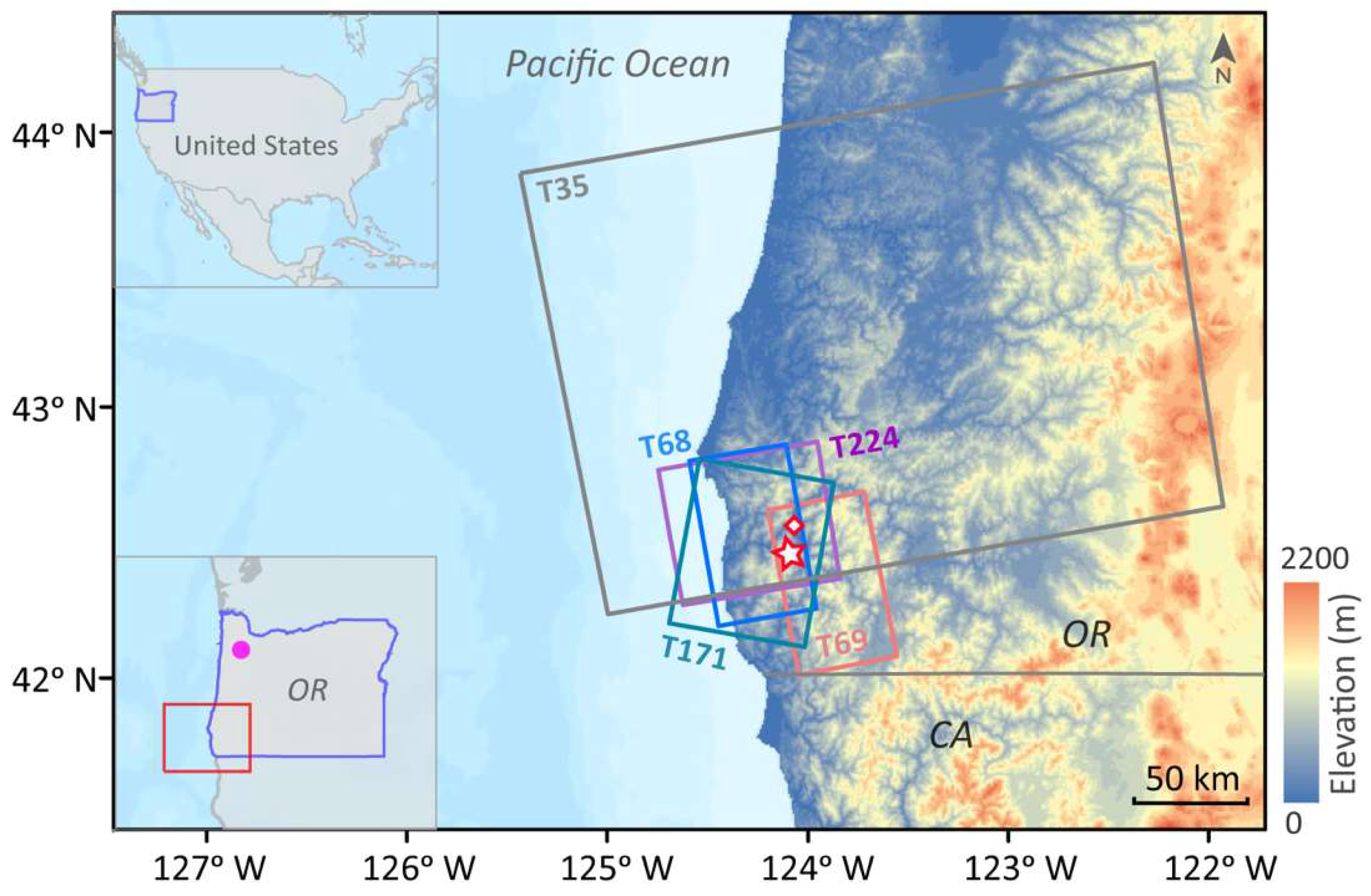
2. Landslide Location and Geological Settings

The Lawson Creek landslide is a slow-moving translational landslide located in southwestern Oregon with a ~1.5 km long and ~500 m wide sliding body (Figure 1). The slope faces northwest with an aspect of ~294° clockwise from north, and the average slope is ~10°. There are no obvious scarps near the landslide’s head as it has been seated on deposits of a previous landslide, and the currently active slide is only a small part of the ancient landslide deposits mapped in the Statewide Landslide Information Database for Oregon (SLIDO [19], Figure S1). The bedrock of the slide is composed of marine sedimentary rocks with sandstone/mudstone lithologies at the upper section, metamorphic rocks with majorly serpentine at the middle section, and metamorphic rocks with phyllite/schist lithologies at the lower section (Figure S2). The toe of the landslide enters Lawson Creek at an elevation of 358 m, and its crown stands at 610 m. The primary precipitation in this region falls between mid-October and mid-April, while little rainfall comes in other months. Moderately dense vegetation covers the landslide site.

3. Materials and Methods

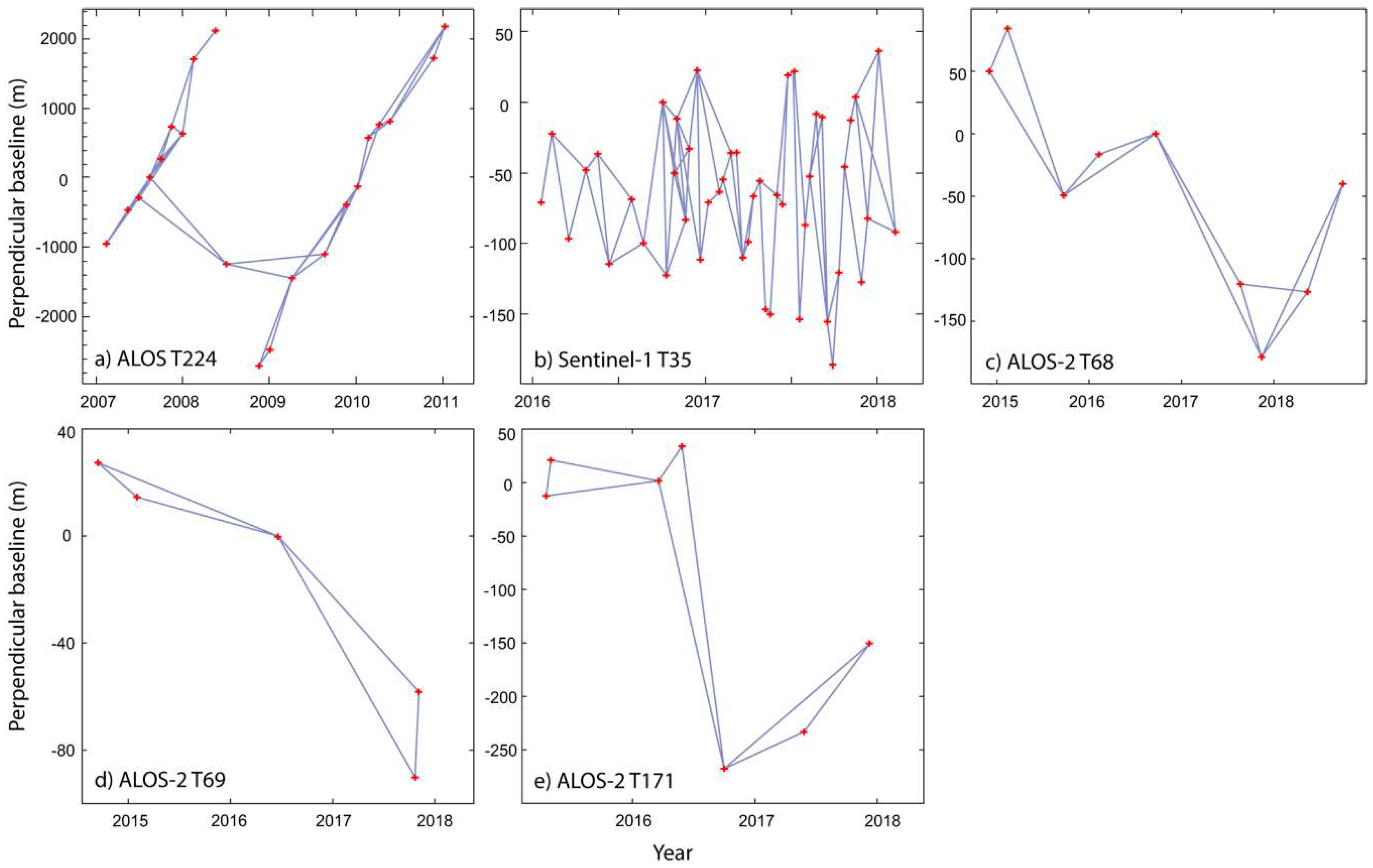
3.1. SAR Interferometry for Landslide Time-Series Mapping

SAR imagery from the ALOS ascending track T224, ALOS-2 ascending tracks T68 and T69 and descending track T171, and the Sentinel-1A/B ascending track T35 were used to map displacements of the Lawson Creek landslide (Figure 1;

Table 1. Spaceborne SAR datasets and usages.

Radar Satellites	Tracks	Flying Directions	Time Span	Usages
Sentinel-1A/B	T35	Ascending	2016–2018	Time-series mapping/surface velocity inversion
ALOS	T224	Ascending	2007–2011	Time-series mapping
ALOS-2	T68	Ascending	2015–2018	Time-series mapping/surface velocity inversion
	T69	Ascending	2014–2018	Surface velocity inversion
	T171	Descending	2015–2018	Surface velocity inversion

). The 1-acrsec Shuttle Radar Topography Mission (SRTM) Digital Elevation Model (DEM) obtained from U.S. Geological Survey (USGS) was used in the InSAR processing. Baseline error and stratified atmospheric artifacts were removed before phase unwrapping. The GAMMA software [20] was used for interferogram generation, phase unwrapping, and removal of stratified atmospheric artifacts. Unwrapping errors in a few interferograms caused by high-gradient sliding movements were corrected by separating the original wrapped phase into an estimated high-gradient displacement component and a residual-phase component (within 2π variation). We unwrapped only the residual-phase component and added it back to the estimated high-gradient component to obtain the final unwrapped phase. The high-gradient displacement component was estimated based on interferograms with short temporal baselines and very good coherence. The corrected interferograms have been listed in the supplementary table.

SAR acquisitions from the ALOS T224 and the Sentinel-1A/B T35 were used to generate time-series displacement maps of the landslide, as they provide temporally dense and coherent observations that allow construction of a fully connected network for time-series inversions (Figure 2). To verify the C-band sentinel-1A/B time series measurements, we also produced results using the L-band ALOS-2 T68 images spanning the same time period (Figure 4d). The full set of interferograms that contain moderate or better coherence (over 0.2 for C-band data and over 0.4 for L-band data) were used for time-series maps: 36 interferograms from the ALOS T224, 5 from the ALOS-2 T68, and 73 from the Sentinel-1A/B T35 (Figure 2) were selected and processed based on the coherence-weighted small baseline subset (SBAS) method [4,21].

Annual deformation rates in LOS (line of sight) directions from the three ALOS-2 tracks and the Sentinel-1A/B track T35 were generated with the stacking method for deriving 3D surface velocity fields of the landslide (

Table 2. Saturated hydraulic conductivity for soils with low bulk density (data modified from [33]).

Soil Types	Data Samples	Saturated Hydraulic Conductivity (m/s)
		25% Quartiles	75% Quartiles	Geometric Mean
Silt loam	58	3.6 $\times$ 10−6	2.8 $\times$ 10−5	1.0 $\times$ 10−5
Silty clay loam	18	1.2 $\times$ 10−6	1.6 $\times$ 10−5	6.7 $\times$ 10−6
Clay loam	17	4.2 $\times$ 10−6	1.6 $\times$ 10−5	7.5 $\times$ 10−6
Sandy loam	127	6.6 $\times$ 10−6	4.1 $\times$ 10−5	1.8 $\times$ 10−5
Silty clay *	-	1.4 $\times$ 10−6–4.2 $\times$ 10−7

* from National Soil Survey Handbook.

), as these data overlap almost the same time period and provide observations with different LOS geometries.

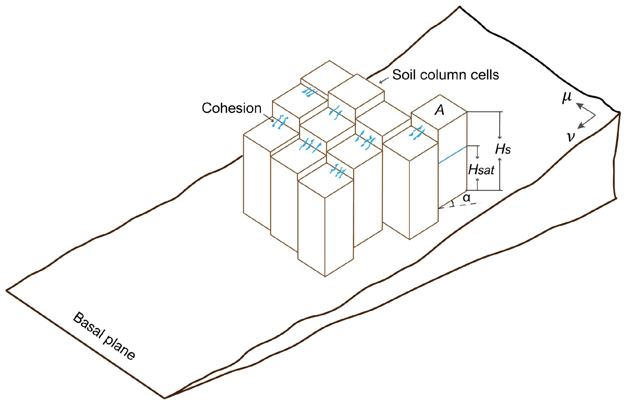
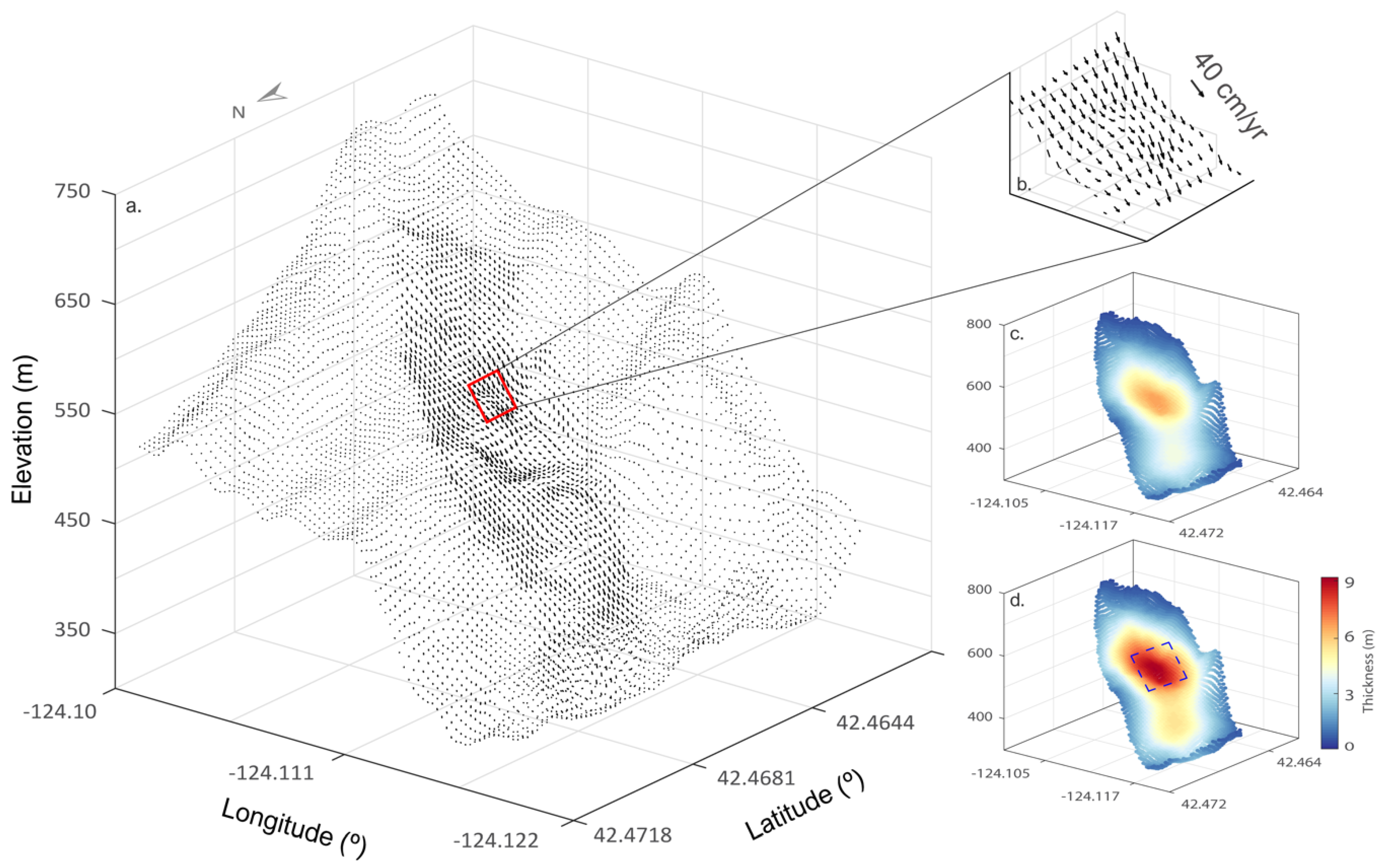
3.2. Thickness Inversion

Constraining the basal depth of a landslide is critical for characterizing movement and estimating the sliding volume. The landslide thickness inversion is achieved by using the surface velocity field obtained from InSAR measurements and applying the principle of mass conservation with assumptions about the variation of the landslide velocity field below the surface [22]:

$$w=\nabla ·\left(f{\mathit{u}}_{surf}h\right)+u_{surf}\cdot \nabla h$$

(1)

where $w$ is the vertical component (outwardly perpendicular to the basal plane as positive) of surface velocity vectors, ${\mathit{u}}_{surf}$ the surface horizontal components, and ℎ the landslide thickness. $f=\left(3-Y/P\right)/3$ is a constant between 0 and 1 depending on landslide rheology, where $Y$ and $P$ are the thickness of the yield zone and the overlaying plug region, respectively [22]. f = 1/2 is consistent with a linear vertical velocity profile, f = 2/3 with Newtonian viscous flow, 2/3 < f < 1 with plug flow, and f = 1 with a rigid sliding block [10]. Equation (4) can be converted to matrix form with finite difference approximations:

$$w_{i,j}=u_{i,j}\frac{f{h}_{i+1,j}-f{h}_{i-1,j}}{\Delta x}+v_{i,j}\frac{f{h}_{i,j+1}-f{h}_{i,j-1}}{\Delta y}+f{h}_{i,j}(\frac{u_{i+1,j}-u_{i-1,j}}{2\Delta x}+\frac{{\nu }_{i,j+1}-{\nu }_{i,j-1}}{2\Delta y})$$

(2)

where $\Delta t$ is the time increment, $u$ and $v$ are surface velocity vectors (Figure 3), $\Delta x$ and $\Delta y$ are grid sizes in $u$ and $v$ direction, respectively, and subscripted $i$ and $j$ are indices in $u$ and $v$.

The surface velocity field can be derived from LOS observations of InSAR, yet reconstructing 3D surface velocity vectors requires at least three independent measurements. In this study, assuming that the sliding body only moves along the downslope direction on the slip plane (i.e., $u$ = 0) [23,24], we construct a pseudo three-dimensional velocity field using the LOS velocities from the ALOS-2 ascending tracks T68 and T69, ALOS-2 descending track T171, and Sentinel-1A/B ascending track T35. Defining $\theta$ as the radar look angle, $\varphi$ the satellite heading angle, $\alpha$ the slope angle, $\beta$ the slope aspect, and $w$ a vector perpendicular to the slope surface defined by vectors $u$ and $v$, the surface velocity field $\mathit{V}={\left[u, v, w\right]}^T$ of each point is related to LOS measurements as:

$$\left[\begin{array}{c}\mathit{l}\\ c_v\end{array}\right]·s·\mathit{V}=\left[\begin{array}{c}\mathit{L}\mathit{O}\mathit{S}\\ 0\end{array}\right]$$

(3)

where $\mathit{l}={\left[l_1,l_2,l_3,\cdots l_k\right]}^T$ is the radar look vector of $k$ independent LOS observations, and $l_1=l_2=\cdots =l_k={\left[-\sin \theta \sin \varphi \sin \theta \cos \varphi -\cos \varphi \right]}^T$, $c_v=\left[-\sin \beta \cos \beta 0\right]$ is the constrain condition, $\mathit{L}\mathit{O}\mathit{S}$ is the $k$ independent InSAR measurements, and $s$ is a coordinate transformation matrix:

$$s=\left[\begin{array}{c}\cos \beta \cos \alpha \sin \beta \cos \alpha -\sin \alpha \\ -\sin \beta \cos \beta 0 \\ \cos \beta \sin \alpha \sin \beta \sin \alpha \cos \alpha \end{array}\right]$$

(4)

We solve Equation (3) to obtain the pseudo 3D surface velocity vectors with the least squares approach, and solve Equation (2) for $h$ by using a nonnegative least squares method [10,25] and setting boundary conditions that the landslide’s thicknesses range from 0 to 200 m and non-landslide regions have a thickness of zero.

3.3. Time Lags

The initiation of seasonally active landslides typically begins days to several weeks after the wet season has arrived [17]. This time lag characterizes how fast the basal pore-air pressure responds to an intense rainfall event, and is jointly controlled by several factors, including the hydraulic conductivity/diffusivity of the landslide material, the landslide thickness, and the rainfall intensity [3,26]. Assuming the top soil layers have been unsaturated because of considerable water loss during dry summers, water infiltration (advective flow) in the top layers is controlled by unsaturated hydraulic conductivity $K$, which is related to the corresponding saturated hydraulic conductivity $K_{sat}$ as [27]:

$$K=K_{sat}{S}_e{}^L{\left\{1-{\left[1-S_e{}^{\frac{n}{n-1}}\right]}^{1-\frac{1}{n}}\right\}}^2$$

(5)

where $L=$ 0.5 is an empirical parameter [28], $n=$ 2 is a measure of pore-size distribution [27], and the effective saturation $S_e$ is calculated as

$$S_e=\frac{\theta -{\theta }_r}{{\theta }_s-{\theta }_r}$$

(6)

with the measured volumetric soil moisture $\theta$, the residual water content ${\theta }_r$, and the saturated water content ${\theta }_s$. Assuming that the landslide consists of multiple homogenous soil layers, the time lag $T_K$ for surface water vertically infiltrating to depth $H_s$ is given as:

$$T_K={\Sigma }_1^m\left(R_i/K_i\right)$$

(7)

where $R_i$ and $K_i$ are the thickness and the hydraulic conductivity of the $i$-th layer, respectively, and the sliding body comprises $m$ soil layers. In saturated soils, an approximately diffusive process would dominate pore pressure responses. The time scale $T_D$ for pore pressure to diffuse vertically downward for depth $H$ is given by

$$T_D=H^2/D_0$$

(8)

where $D_0$ is the hydraulic diffusivity. Advective water flow is slower than hydraulic diffusion, and they together control the response time of basal pore pressure to rainfall events if the groundwater level is between the basal plane and the ground surface.

3.4. Failure Depth Using Limit Equilibrium Analysis

Slope stability evaluation is implemented based on the Mohr-Coulomb shearing failure criterion. Assuming that the hillslope consists of soil columns with cross-section area $A$ and height $H_s$, and cohesion $c$ exists among column cells [29] (Figure 3). Because of the self-gravity, a vertical force $F_G$ is posed on the base of each soil column:

$$F_G=Mg=A{H}_S\left[\theta \rho w+\left(1-\varphi \right){\rho }_s\right]g$$

(9)

where $M$ is the mass of each soil column, $g$ the gravity of earth, $\theta$ the volumetric water content, ${\rho }_w$ the density of water, ${\rho }_s$ the bulk density of soil, and $\varphi$ the porosity of soil.

Relating $F_G$ to the cross-section area of soil columns along the slope $A/\cos \beta$, $F_G$ can be decomposed into normal stress ${\sigma }_N$ and downslope driving component ${\sigma }_d$:

$${\sigma }_N=\frac{F_N}{A/\cos \alpha }=\frac{F_G\cos \alpha }{A/\cos \alpha }=H_S[\theta {\rho }_W+(1-n){\rho }_s]g{\cos }^2\alpha$$

(10)

$${\sigma }_d=\frac{F_d}{A/\cos \alpha }=\frac{F_G\sin \alpha }{A/\cos \alpha }=H_S[\theta {\rho }_W+(1-\varphi ){\rho }_s]g\sin \alpha \cos \alpha$$

(11)

where $F_N$ is the counteracting normal force, $F_d$ the downslope driving force, and $\alpha$ the slope angle. When perched water table reaches height $H_w$, the resisting forces ${\tau }_f$ are reduced as the pore pressure $u_w$ weakens the effective stress ${\sigma }_e$ by $u_a=H_w{\rho }_{w}g{\cos }^2\alpha$ under saturated conditions

$${\tau }_f=c+{\sigma }_e\tan \gamma =c+\left({\sigma }_N-u_w\right)\tan \gamma$$

$$=c+\left\{H_s\left[\theta {\rho }_w+\left(1-\varphi \right){\rho }_s\right]g{\cos }^2\alpha -H_w{\rho }_{w}g{\cos }^2\alpha \right\}\tan \gamma$$

(12)

Slope failures occur when driving force ${\sigma }_d$ exceeds shearing resistance ${\tau }_f$. We can obtain $H_w$ as a function of $H_s$ using the critical condition ${\sigma }_d={\tau }_f$

$$H_w=-\frac{\theta {\rho }_w+\left(1-\varphi \right){\rho }_s\cos \alpha \left(\sin \alpha -\cos \alpha \tan \gamma \right)}{{\rho }_{w}g{\cos }^2\alpha \tan \gamma }{H}_s+\frac{c}{{\rho }_{w}g{\cos }^2\alpha \tan \gamma }$$

(13)

$H_w$ is a monotonically increasing function with respect to $H_s$ if $\alpha <\gamma$, as $\frac{d{H}_w}{d{H}_s}>0$. Moreover, $H_w$ must be less than or equal to $H_s$ as overland flow would form when $H_w>H_s$. Letting $H_w=H_s$ yields the maximum height that a saturated soil column can maintain stable without shearing failure.

Under unsaturated soil conditions, soil strength is enhanced by ${\tau }_h$ because of the capillary pressure. The shearing resistance ${\tau }_f$ can be expressed as

$${\tau }_f=c+\left\{H_s\left[\theta {\rho }_w+\left(1-\varphi \right){\rho }_s\right]g{\cos }^2\alpha -{\tau }_h\right\}\tan \gamma$$

(14)

$${\tau }_h={\rho }_{w}g\left|h_c{S}_e\right|={\rho }_{w}g\left|h_b{S}_e{}^{1-1/\lambda }\right|$$

(15)

with capillary pressure head $h_c$, air-entry value $h_b$, pore size distribution parameter $\lambda$ [30], and effective saturation $S_e$.

4. Results

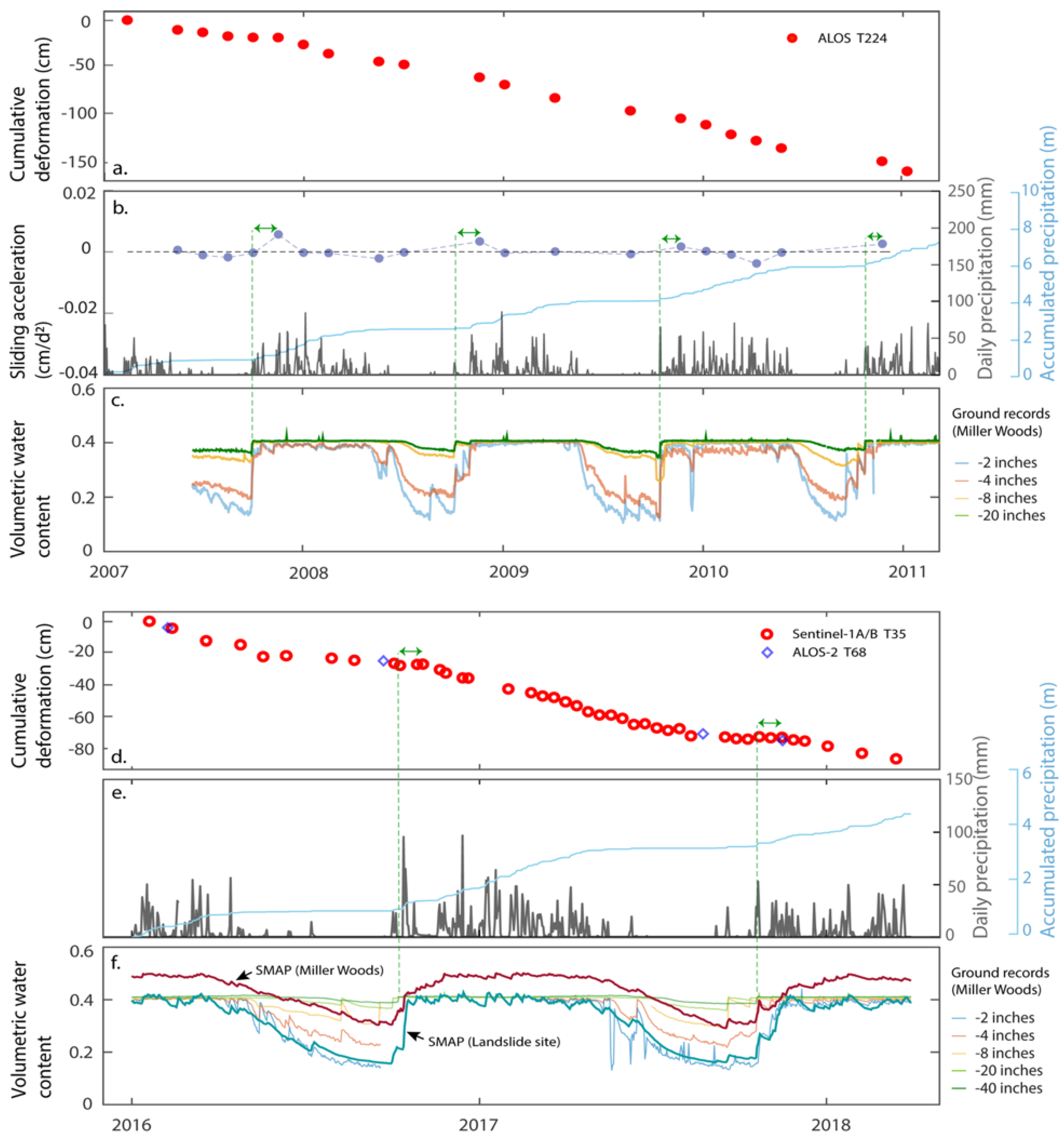
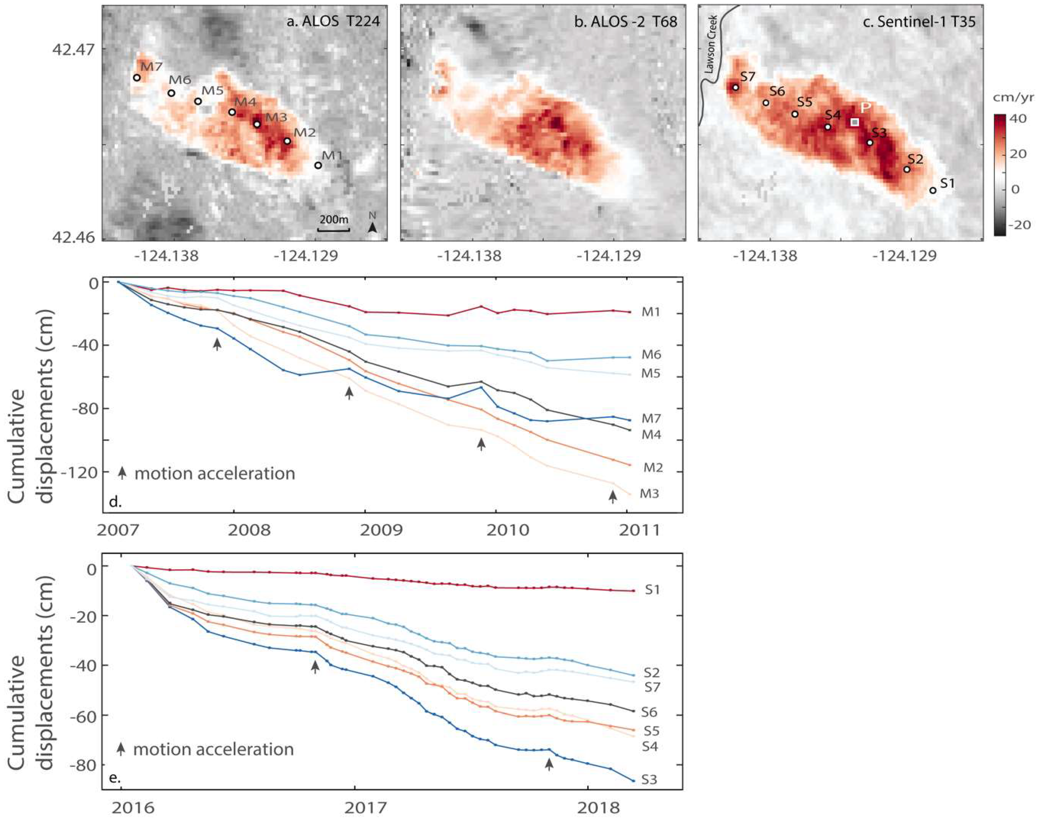
4.1. Time-Series Displacements and Annual Deformation Rates

From 2007 to 2011, sliding movement of the Lawson Creek landslide is captured by SAR data from the ALOS ascending track T224. Figure 4a illustrates the time-series displacements of a typical fast-moving point $\mathrm{P}$ (Figure 5c) between 2007 and 2011. As the measurement of one single pixel can be easily contaminated by noises, we averaged the time-series deformation of the 3 $\times$ 3 array of adjacent points, which corresponds to a 60 m $\times$ 60 m area on the landslide surface. Similarly, we mapped time-series displacements of the same point from 2016 to 2018 using imagery from the Sentinel-1A/B ascending track T35, and from the ALOS-2 ascending track T68 for cross-validation. The results show that both the L-band ALOS-2 and the C-band Sentinel-1A/B datasets produce highly similar results (Figure 4d). The cumulative downslope displacement of the slide is about 1.5 m from 2007 to 2011 and around 0.8 m from 2016 to 2018, and movement patterns resemble an annual cycle throughout the years: the sliding motion starts to accelerate after wet seasons arrive and decelerates substantially when summer comes; while a considerable amount of deformation occurs from mid-November to mid-May, few displacements appear during the dry seasons from mid-May to mid-November (Figure 5d,e). Nevertheless, the landslide movement does not totally stop even during dry summers; similar behaviors have been observed at other landslides over the pacific northwest [5,23].

The map of annual deformation rates show that the Lawson creek landslide had been moving downslope at almost the same rates (maximum 40 cm/yr) with spatially similar patterns during the two separate observation periods (Figure 5a,b and Figure S3). It has been continuously creeping for the past decade. Specifically, the middle section presents much faster movements than both the landslide head and toe sections. It is worth noting that, despite the spatial differences in movement rates, all the points on the landslide surface demonstrate a highly similar trend on the temporal axis. As shown in Figure 5d,e, the points in varied locations present apparent seasonal accelerations on the same dates near mid-November.

4.2. Time Retardation to Seasonal Precipitation

To further characterize the dynamic behavior of the landslide responding to season changes, we used the point $\mathrm{P}$ as a representative and employed the finite-difference formula to obtain the acceleration of its motions:

$$a_j=\frac{2\left(v^{+}-v^{-}\right)}{t_{j+1}-t_{j-1}}$$

(16a)

$$v^{+}=\frac{d_{j+1}-d_j}{t_{j+1}-t_j}$$

(16b)

$$v^{-}=\frac{d_j-d_{j-1}}{t_j-t_{j-1}}$$

(16c)

where $d_j$ and $a_j$ represent, respectively, the cumulative displacement and the acceleration of the point $\mathrm{P}$ at time $t_j$. $v^{-}$ and $v^{+}$ represent the deformation rates. Seasonal landslide movements start when $a_j>$ 0. For the temporally dense Sentinel-1A/B measurements, recognizing onset dates of the seasonal movements is easy and straightforward through visual interpretation (Figure 4d), while for the temporally sparse ALOS T224 results, the finite-difference method is applied to determine the dates when seasonal sliding commence every year. Note that though there are several visible motion accelerations from the Sentinel-1A/B displacement time series, here we only focus on the most noticeable seasonal acceleration, namely, the first wet-season acceleration in around mid-November after a continuous summer deceleration.

As shown in Figure 4b,e, although the wet-season arrives in mid-October regularly every year, the landslide does not begin to accelerate until several weeks later, generally in November. However, the exact time lags vary by years. The maximum values stand at 41 days, 41 days, 31 days, 26 days, 43 days, and 37 days for 2007, 2008, 2009, 2010, 2016, and 2017 respectively (Figure 4a,d) as the displacements might happen before the date when satellites capture the deformation. The 46-day revisit cycle of the ALOS acquisitions cannot provide an effective lower bound to the time lags for years 2007–2011, but the Sentinel-1A/B datasets with a minimum revisit period of six days successfully set the lower boundaries to 25 days for both years 2016 and 2017. As the landslide always accelerates after the arrival of wet-seasons (i.e., the theoretical lower boundary is 0 day), the time lag ranges are 0–41 days, 0–41 days, 0–31 days, 0–26 days, 25–43 days, and 25–37 days for 2007, 2008, 2009, 2010, 2016, and 2017, respectively.

Every year, the soil moisture gradually falls to a year low in the summer and rises back to a high level as the wet-season approaches, and it maintains at this high level until the next summer comes (Figure 4c,f). Here we define the arrival date of wet seasons as when the 40-inch-depth (~1 m) soil moisture at the Miller Woods station rises back to the same level as previous wet seasons, based on the assumption that a few slight early-autumn rainfall events can hardly mark the coming of wet seasons. In other words, the top 40-inch soils have been saturated.

There is a three-fold justification for using soil moisture records from the Miller Woods station to represent for the landslide site. First, both sites undergo almost the same rainfall events as revealed by the SMAP soil moisture acquisitions at these two sites. As illustrated in Figure 4f, each rise of the fluctuated SMAP soil moisture can be interpreted as a distinguishable rainfall event, and SMAP data at both sites constantly exhibit such rise responses at the same dates. It is worth noting that SMAP soil moisture data used here are captured by satellites independently. The values are the mean soil moisture of the top 5-centimeter soil layers, thus even slight rainfall events can lead to a rising fluctuation on the SMAP data. Second, both sites have similar soil layer compositions. Soils at the Miller woods station constitute layers of silt loam (0–16 cm depth), silty clay loam (16–33 cm), silty clay (33–63 cm), and gravelly clay loam (63–152 cm). These soil layers have similar saturated hydraulic conductivity as that at the landslide site, which comprise of channery loam (0–30 cm), silt loam (30–56 cm), silty clay loam (56–74 cm), sandy loam (74–158 cm), and silty clay loam (158–183 cm) (from NCSS soil pedons [31] and local surveys [32]). Calculating infiltration time of the top 40-inch soils at both sites using Equation (7) and the mean hydraulic conductivities in Table 2 shows that the landslide site would respond earlier than the Miller Woods by only 3.7 days. Third, soil moisture measured at the Miller Woods ground station matches well with the SMAP acquisitions in terms of rainfall responses though the absolute value varies; however, here only the post-summer soil moisture rise was used rather than the absolute value to determine the dates.

Be aware that the SMAP data which represent average volumetric water contents of the top 5 cm soils are sensitive to any sight rainfall events, thus it is helpful to refer to the ground soil moisture at the 40-inch level to determine the dates according to our definition of the arrival of wet-seasons. An alternate empirical approach is thresholding SMAP soil moisture by a 25% post-summer rise in that year, that is:

$$\frac{{\theta }_{thresh}-{\theta }_{min}}{{\theta }_{max}- {\theta }_{min}}=25\%$$

(17)

where ${\theta }_{max}$ is the mean SMAP soil moisture during the wet season, ${\theta }_{min}$ is the minimum SMAP soil moisture in the summer, and the arrival date of the wet season can be determined when the SMAP soil moisture rises back to ${\theta }_{thresh}$ after a dry summer. For years 2016 and 2017, this method can produce the same results with an uncertainty of 2 days as using the ground-truth data.

Soil moisture records at the 40-inch depth of the Miller Woods station are unavailable from 2007 to 2011, therefore, the corresponding time lags are calculated by using soil moisture data at the 20-inch depth and adding on extra 5 days. The extra days are the observed time interval between successive soil moisture surges at the 20-inch and 40-inch depths right after the 2016 and 2017 summers, which represent the water infiltration time from the 20-inch to the 40-inch depths (Figure 4f).

4.3. Basal Depths and Volume Inferred from InSAR Observations

Annual displacement rates from two ALOS-2 ascending tracks T68 and T69, one descending track T171, and one Sentinel-1A/B ascending track T35 were employed to derive the 3D surface velocity fields of the landslide (Table 1; Figure 5 and Figure S3). As the observations from the three ascending tracks are not highly independent because of the similar LOS directions, we constrain the landslide motions to be along-slope to achieve stable inversions. The 3D surface velocity vectors are shown in Figure 6a,b.

Thickness inversion of surface points corresponding to every SAR-interferogram pixel (20 m $\times$ 20 m) were implemented by using the mass conservation approach and assuming a power-law rheology as Equation (1). Here the yield slope-perpendicular depth of each pixel has been converted to vertical thickness (Figure 6c,d). The thickness map shows that the sliding plane at the middle and upper sections are seated deepest, with a maximum mean basal depth of the central region as 5.8 m to 7.8 m (Figure 6c,d), assuming the landslide is characterized by a plug flow (2/3 $<f<$ 1) as suggested by borehole measurements of multiple slow-moving landslides [22,34,35,36,37,38,39]. The basal plane has an upwardly concave shape that exhibits greater thickness in the central and gradually shallows to the margin area.

The uncertainty caused by the $u=0$ assumption can be largely quantified by defining $u=kv$, where $k$ is a constant mediating movement direction of the landslide. The constraint in Equation (3) is modified to $c_v=\left[\begin{array}{ccc}k\cos \beta +\sin \beta & k\sin \beta -\cos \beta & 0\end{array}\right]$, accordingly. Letting $k=\pm 0.2$ is equivalent to varying the landslide movement direction by $11°$, which yields mean basal depths of the central region as 4.3 m to 6.9 m for $f=1$, and 6.0 m to 9.5 m for $f=2/3$. Taking into account the uncertainties, the estimated basal depth is expanded to $6.9\pm 2.6$ m. Then, the estimated volume of the sliding body ranges from 2.9 $\times$ 10⁶ to 5.9 $\times$ 10⁶ m³.

4.4. Failure Depths from Limit Equilibrium Analysis

Basal geometry inversions illustrate that the landslide body is thick in the central section yet shallow in the head and toe sections. However, it remains unclear whether the initial rainfall-triggered motions start from the shallow sections or commence from the thickest central section. The limit equilibrium analysis was implemented to obtain the theoretical initial failure depth.

Slope failures may occur under both saturated and unsaturated soil conditions [17,40]. Mohr-Coulomb failure criterion is applicable to both cases for slope stability evaluation:

$${\tau }_f=c+{\sigma }_e\tan \gamma$$

(18)

where ${\tau }_f$ is the limit shear strength, $c$ the effective cohesion, $\gamma$ the internal friction angle, and ${\sigma }_e$ the effective stress. Slopes failures occur when the driving force along the downslope direction ${\sigma }_d$ exceeds the limit shear strength ${\tau }_f$.

Limit equilibrium analysis of the landslide in an unsaturated condition (Equations (14) and (15)) with parameters from [41] demonstrates that shearing failures cannot occur unless the soil moisture is over 0.39, yet soil moisture records (SMAP satellite acquisitions and ground records) at both the Miller Woods station and the landslide site suggest that soil moisture at the landslide site is less than 0.35 during summers. Therefore, the seasonal movement of the landslide is initiated by shear failures of saturated soils.

Geotechnical logs of a nearby 69-feet deep water well (CURR 1286) suggests that the shearing zones of the Lawson Creek landslide is primarily composed of brown clay. As detailed soil mechanical parameters are unavailable, the uncertainties are accounted by expanding the parameter range to include soils ranging from silty clay to clay based on global laboratory and field tests: internal friction angle $\gamma =29\pm 7°$ and cohesion $c=12\pm 3$ kpa [32,42,43,44,45,46,47,48]. The slope angles of the landslide on the basal surface is less than 15$°$. Using the measured volumetric water content $\theta =$ 0.41 during wet-seasons and soil porosity $\varphi =$ 0.47 [41], we can obtain the critical basal depth $H_c=7.6\pm 1.6$ m where shearing failures would commence using Equation (13), based on the Mohr-Coulomb failure criterion. This result agrees well with the InSAR-inferred basal depth of $6.9\pm 2.6$ m, which confirms the correctness of the inverted thickness based on mass conservation and surface velocities. Meanwhile, it indicates that the deep-seated central region is close to stress equilibrium when the soils are fully saturated, and a slight pore pressure rise would trigger the motion acceleration. Note that the landslide had motions even during the dry summer, while intermittent post-summer rainfall did not cause simultaneous motion acceleration (Figure 4), implying that the seasonal acceleration is caused by pore pressure rise rather than loading from rainwater.

4.5. Potential for Estimating Hydraulic Parameters

Taking into account the uncertainties caused by SMAP data (±2 days) and soil compositions (−3.7 days), the time lags of 25–43 days observed from satellite remote sensing is expanded to 26.7–48.7 days. With the known time lags and InSAR-inferred basal depth of $6.9\pm 2.6$ m, the rainwater infiltration rate can be quantified. Here the time lags stand for water infiltration from the 40-inch depth to the initial failure depth.

As groundwater level decreases during the dry summers, initial wet-season precipitation must saturate the top soil layers via advective flow first before the hydraulic diffusion process takes control of the basal pore-pressure response. The averaged hydraulic conductivity of soil layers above the groundwater table and the averaged hydraulic diffusivity below the table can both be effectively quantified with the given groundwater levels. However, such data is not available for this case study and therefore only the upper and lower bound of the hydraulic parameters can be estimated.

Assuming the groundwater table is below the basal plane leads to an estimate of characteristic hydraulic conductivity $K_s$ (upper bound) as 2.4 $\times$ 10⁻⁵ m/s using Equations (5) and (7), whereas assuming fully saturated soils yields an estimated characteristic hydraulic diffusivity $D_0$(lower bound) as 2.6 $\times$ 10⁻⁶ m²/s using Equation (8). Note that here characteristic hydraulic conductivity/diffusivity means to treat a soil column that constitutes multiple heterogeneous layers as one single soil sample.

Employing empirical relationship between $K_s$ and $D_0$ of the same soils can provide the other bounds for the estimations. The vertical soil profile of the Lawson Creek landslide comprises boulders and clay brown, clay brown, and clay blue layers from the nearby water well log (CURR 1286). We interpret the characteristic hydraulic conductivity as similar to that of silty clay and obtain an empirical approximation as $D_0={10}^2\cdot K_s$ [16,49]. It can yield a lower bound for the $K_s$ as 2.6 $\times$ 10⁻⁸ m/s and an upper bound for $D_0$ as 3.7 $\times$ 10⁻⁴ m²/s. Accordingly, combining both approaches can bound the characteristic hydraulic conductivity to (2.6 $\times$ 10⁻⁸, 2.4$\times$ 10⁻⁵) m/s and the characteristic hydraulic diffusivity to (2.6 $\times$ 10⁻⁶, 3.7$\times$ 10⁻⁴) m²/s. The average is given as $K_s$ = 1.2 $\times$ 10⁻⁵ m/s and $D_0$= 1.9 $\times$ 10⁻⁴ m²/s. Given the fact that even field-measured hydraulic conductivity has an uncertainty by 10³ m/s [15,16], the above-described estimations is of important practical value.

5. Discussion

In this investigation, basal depth inversion of the landslide is achieved based on mass conservation and InSAR-captured surface velocity. A $u=0$ (Figure 3) assumption is employed to reconstruct the 3D surface velocity field, as currently spaceborne SAR images can only provide two independent LOS observations. This assumption largely agrees with the landslide behavior monitored by continuous GPS (global positioning system) at several sites [23,50] and can provide a reasonable estimation of the thickness distribution over the whole landslide area, as confirmed by the uncertainty analysis and by the independent limit equilibrium analysis by feeding a wide range of soil mechanical parameters. Besides, it is worth noting that the selected wide range of rheological parameter ($2/3<f<1$) has also partly compensated the uncertainty derived from the 3D surface velocity reconstruction.

Determining the starting date of the wet season is a key difficulty in estimating time lags. Thresholding cumulative precipitation is one of the options. However, analyzing cumulative rainfall from summer to the date of the first motion acceleration reveals that there are significant variations by years. For instance, the cumulative precipitation stands at 290 mm, 256 mm, 232 mm, 341 mm, 381 mm, and 336 mm for year 2007, 2008, 2009, 2010, 2016, and 2017, respectively (Figure 4b,e), which can hardly lead to a reliable and accurate threshold value. In situ precipitation data show that the first several post-summer rainfall events are generally intermittent, while a single rainfall event cannot represent the arrival of wet-seasons. Cumulative rainfall infiltrates into the basal plane to trigger seasonal landslide motions, yet a single rainfall with a short duration and a small intensity is unlikely to saturate the entire sliding material and raise pore pressure on the basal plane. In contrast, the soil moisture that reflects the degree of saturation of soils can thus be a good indicator to define the starting date of wet seasons.

The lack of in situ measurements such as groundwater level from this far-away landslide site has posed challenges to the hydraulic parameter estimation. Hence, only lower and upper bounds for characteristic hydraulic conductivity and diffusivity are estimated. To account for all related uncertainties, the average basal depth of the central landslide region is used, rather than a single point. The derived time lags also have included the uncertainties that stem from satellite revisit cycle and varied soil moisture methods and locations. Because of the limited field data, here we only aim to layout a framework for estimating landslide thickness and corresponding hydraulic parameters, and better results can be obtained if more field data are available.

Regarding SAR datasets for landslide studies, L-band data overall exhibit better coherence on vegetated terrains than C-band data, while the C-band Sentinel-1 imagery has unique advantages on time-series mapping because of the dense temporal acquisitions. The free ALOS and Sentinel-1 images have greatly contributed to the data availability between 2007 and 2011 and after 2015, and the gap between 2011 and 2015 might be filled with commercial SAR datasets. Currently, spaceborne SAR datasets can only provide two independent observations, yet incorporating data from airborne missions such as Uninhabited Aerial Vehicle SAR (UAVSAR [51]) is a potential solution to obtain the three-dimensional surface velocity field of a landslide.

The Lawson Creek landslide is a typical slow-moving slide that is seated on the deposit of an ancient landslide (>150 years [19]). The slow-moving behavior is very likely attributed to the soil porosity [52], yet the seasonal dynamics are primarily associated with precipitation. InSAR observations reveal that the central region has greater displacement rate than the toe and head sections. These imply that the central area is the active part, while movements of the landslide head and toe might be passive. During the past decade, the moving rate has been slow and stable, and currently no sign of runout is present.

6. Conclusions

This investigation employs multiple SAR datasets including ALOS, ALOS-2, and Sentinel images spanning 2007–2011 and 2016–2018 to map time-series displacement of a translational landslide in the southern Oregon, which reveals that the landslide has been continuously creeping for the whole past decade with a maximum rate of 40 cm/yr in the upper middle section. The landslide motion exhibits apparent seasonal patterns with considerable displacements during wet seasons from mid-November to mid-May while little deformation during dry summers. The basal depth of the landslide is inverted based on the mass conservation theory and InSAR-inferred surface velocity fields by assuming a power-law rheology. The results show that the Lawson Creek landslide is seated deepest in the central region and gradually shallows to the margin area. The mean thickness of the central region stands at $6.9\pm 2.6$ m. This estimation is also validated and confirmed by an independent limit equilibrium analysis which demonstrates that initial shearing failure of saturated soil columns would occur at $7.6\pm 1.6$ m depth.

The time lags between the arrival of wet seasons and the onset of seasonal landslide motions are determined based on the observed periodic post-summer rise of soil moisture (SMAP and ground records) and InSAR time-series measurements. During the observation period, the time lags range from 26.7 to 48.7 days including uncertainties. InSAR observations reveals that the landslide kept moving even during dry summers and intermittent post-summer rainfall did not cause simultaneous acceleration of landslide motion, implying that seasonal accelerations are caused by basal pore-pressure rise rather than loading of rainwater. Accordingly, we take the water infiltration as purely advective flow and purely water diffusion respectively to estimate the lower and upper bounds of the characteristic hydraulic conductivity $K_s$ and diffusivity $D_0$ of the landslide material, as groundwater level data are unavailable. The yield average values are $K_s$ = 1.2 $\times$ 10⁻⁵ m/s and $D_0$ = 1.9 $\times$ 10⁻⁴ m²/s.

As with most landslides all over the globe, for the Lawson Creek landslide, in situ measurements of basal depth and hydraulic parameters are unavailable despite their importance for characterizing landslide behaviors. However, here we have explored the possibility of using primarily remote sensing datasets to infer the landslide thickness and estimate the hydraulic conductivity and diffusivity. More importantly, this established framework is able to yield better estimates when extra inputs are available. For instance, thickness inversion can be improved with more than three independent LOS observations, and hydraulic estimations can be enhanced with known groundwater levels.

References

1. Wartman, J.; Montgomery, D.R.; Anderson, S.A.; Keaton, J.R.; Benoît, J.; dela Chapelle, J.; Gilbert, R. The 22 March 2014 Oso landslide, Washington, USA. Geomorphology 2016, 253, 275–288. [Google Scholar] [CrossRef]
2. Iverson, R.M.; George, D.L.; Allstadt, K.; Reid, M.E.; Collins, B.D.; Vallance, J.W.; Schilling, S.P.; Godt, J.W.; Cannon, C.M.; Magirl, C.S.; et al. Landslide mobility and hazards: Implications of the 2014 Oso disaster. Earth Planet Sci. Lett. 2015, 412, 197–208. [Google Scholar] [CrossRef]
3. Hilley, G.E.; Bürgmann, R.; Ferretti, A.; Novali, F.; Rocca, F. Dynamics of slow-moving landslides from permanent scatterer analysis. Science 2004, 304, 1952–1955. [Google Scholar] [CrossRef] [PubMed]
4. Tong, X.; Schmidt, D. Active movement of the Cascade landslide complex in Washington from a coherence-based InSAR time series method. Remote Sens. Environ. 2016, 186, 405–415. [Google Scholar] [CrossRef]
5. Liu, P.; Li, Z.; Hoey, T.; Kincal, C.; Zhang, J.; Zeng, Q.; Muller, J.P. Using advanced InSAR time series techniques to monitor landslide movements in Badong of the Three Gorges region, China. Int. J. Appl. Earth Obs. Geoinf. 2013, 21, 253–264. [Google Scholar] [CrossRef]
6. Jebur, M.N.; Pradhan, B.; Tehrany, M.S. Detection of vertical slope movement in highly vegetated tropical area of Gunung pass landslide, Malaysia, using L-band InSAR technique. Geosci. J. 2014, 18, 61–68. [Google Scholar] [CrossRef]
7. Schlögel, R.; Doubre, C.; Malet, J.P.; Masson, F. Landslide deformation monitoring with ALOS/PALSAR imagery: A D-InSAR geomorphological interpretation method. Geomorphology 2015, 231, 314–330. [Google Scholar] [CrossRef]
8. Nikolaeva, E.; Walter, T.R.; Shirzaei, M.; Zschau, J. Landslide observation and volume estimation in central Georgia based on L-band InSAR. Nat. Hazards Earth Syst. Sci. 2014, 14, 675–688. [Google Scholar] [CrossRef] [Green Version]
9. Aryal, A.; Brooks, B.A.; Reid, M.E. Landslide subsurface slip geometry inferred from 3-D surface displacement fields. Geophys. Res. Lett. 2015, 42, 1411–1417. [Google Scholar] [CrossRef]
10. Booth, A.M.; Lamb, M.P.; Avouac, J.P.; Delacourt, C. Landslide velocity, thickness, and rheology from remote sensing: La Clapière landslide, France. Geophys. Res. Lett. 2013, 40, 4299–4304. [Google Scholar] [CrossRef]
11. Iverson, R.M.; Major, J.J. Rainfall, ground-water flow, and seasonal movement at Minor Creek landslide, northwestern California: Physical interpretation of empirical relations. Geol. Soc. Am. Bull. 1987, 99, 579–594. [Google Scholar] [CrossRef]
12. Reid, M.E. A pore-pressure diffusion model for estimating landslide-inducing rainfall. J. Geol. 1994, 102, 709–717. [Google Scholar] [CrossRef]
13. Baum, R.L.; Reid, M.E. Geology, hydrology, and mechanics of a slow-moving. Clay Shale Slope Instab. 1995, 10, 79. [Google Scholar]
14. Bogaard, T.A.; Greco, R. Landslide hydrology: From hydrology to pore pressure. Wires Water 2016, 3, 439–459. [Google Scholar] [CrossRef]
15. Berti, M.; Simoni, A. Field evidence of pore pressure diffusion in clayey soils prone to landsliding. J. Geophys. Res.-Earth 2010, 115. [Google Scholar] [CrossRef] [Green Version]
16. Berti, M.; Simoni, A. Observation and analysis of near-surface pore-pressure measurements in clay-shales slopes. Hydrol. Process. 2012, 26, 2187–2205. [Google Scholar] [CrossRef]
17. Iverson, R.M. Landslide triggering by rain infiltration. Water Resour. Res. 2000, 36, 1897–1910. [Google Scholar] [CrossRef] [Green Version]
18. Rutt, I.C.; Hagdorn, M.; Hulton, N.R.J.; Payne, A.J. The Glimmer community ice sheet model. J. Geophys. Res.-Earth 2009, 114. [Google Scholar] [CrossRef] [Green Version]
19. Burns, W.J. Statewide Landslide Information Database for Oregon [SLIDO], Release 3.2: Oregon Department of Geology and Mineral Industries, Geodatabase. 2014. Available online: http://www.oregongeology.org/sub/slido (accessed on 30 March 2019).
20. Werner, C.; Wegmüller, U.; Strozzi, T.; Wiesmann, A. Gamma SAR and interferometric processing software. In Proceedings of the ERS-ENVISAT Symposium, Gothenburg, Sweden, 16–20 October 2000; Volume 1620. [Google Scholar]
21. Berardino, P.; Fornaro, G.; Lanari, R.; Sansosti, E. A new algorithm for surface deformation monitoring based on small baseline differential SAR interferograms. IEEE Trans. Geosci. Remote Sens. 2002, 40, 2375–2383. [Google Scholar] [CrossRef] [Green Version]
22. Delbridge, B.G.; Bürgmann, R.; Fielding, E.; Hensley, S.; Schulz, W.H. Three-dimensional surface deformation derived from airborne interferometric UAVSAR: Application to the Slumgullion Landslide. J. Geophys. Res. Solid Earth 2016, 121, 3951–3977. [Google Scholar] [CrossRef] [Green Version]
23. Hu, X.; Lu, Z.; Pierson, T.C.; Kramer, R.; George, D.L. Combining InSAR and GPS to Determine Transient Movement and Thickness of a Seasonally Active Low-Gradient Translational Landslide. Geophys. Res. Lett. 2018, 45, 1453–1462. [Google Scholar] [CrossRef]
24. Cascini, L.; Fornaro, G.; Peduto, D. Advanced low-and full-resolution DInSAR map generation for slow-moving landslide analysis at different scales. Eng. Geol. 2010, 112, 29–42. [Google Scholar] [CrossRef]
25. Grant, M.; Boyd, S.; Ye, Y. CVX: Matlab Software for Disciplined Convex Programming. 2008. Available online: http://cvxr.com/cvx/ (accessed on 1 April 2019).
26. Priest, G.R.; Schulz, W.H.; Ellis, W.L.; Allan, J.A.; Niem, A.R.; Niem, W.A. Landslide stability: Role of rainfall-induced, laterally propagating, pore-pressure waves. Environ. Eng. Geosci. 2011, 17, 315–335. [Google Scholar] [CrossRef]
27. Van Genuchten, M.T. A closed-form equation for predicting the hydraulic conductivity of unsaturated soils. Soil Sci. Soc. Am. J. 1980, 44, 892–898. [Google Scholar] [CrossRef]
28. Mualem, Y. A new model for predicting the hydraulic conductivity of unsaturated porous media. Water Resour. Res. 1976, 12, 513–522. [Google Scholar] [CrossRef] [Green Version]
29. Lehmann, P.; Or, D. Hydromechanical triggering of landslides: From progressive local failures to mass release. Water Resour. Res. 2012, 48. [Google Scholar] [CrossRef]
30. Brooks, R.; Corey, T. Hydraulic Properties of Porous Media. In Hydrology Papers 3; Colorado State University: Fort Collins, CO, USA, 1964; Volume 24, p. 37. [Google Scholar]
31. USDA. Soil Survey of Curry County, Oregon. 1994. Available online: https://www.nrcs.usda.gov/Internet/FSE_MANUSCRIPTS/oregon/OR015/0/Curry.pdf (accessed on 1 April 2019).
32. USDA. National Cooperative Soil Survey Soil Characterization Data. 2019. Available online: https://ncsslabdatamart.sc.egov.usda.gov (accessed on 25 March 2019).
33. Pachepsky, Y.; Park, Y. Saturated hydraulic conductivity of US soils grouped according to textural class and bulk density. Soil Sci. Soc. Am. J. 2015, 79, 1094–1100. [Google Scholar] [CrossRef]
34. Wasowski, J. Inclinometer and piezometer record of the 1995 reactivation of the Acquara-Vadoncello landslide, Italy. In Proceedings of the Engineering Geology: A global view from the Pacific Rim, Vancouver, BC, Canada, 21–25 September 1998; Volume 3, pp. 1697–1704. [Google Scholar]
35. Gould, J.P. A study of shear failure in certain Tertiary marine sediments. In Proceedings of the Research Conference on Shear Strength of Cohesive Soils, Boulder, CO, USA, 13–17 June 1960; pp. 615–641. [Google Scholar]
36. Mainsant, G.; Larose, E.; Brönnimann, C.; Jongmans, D.; Michoud, C.; Jaboyedoff, M. Ambient seismic noise monitoring of a clay landslide: Toward failure prediction. J. Geophys. Res. Earth Surf. 2012, 117. [Google Scholar] [CrossRef] [Green Version]
37. Iverson, R.M. A constitutive equation for mass-movement behavior. J. Geol. 1985, 93, 143–160. [Google Scholar] [CrossRef]
38. Van Asch, T.W.; Malet, J.P.; Bogaard, T.A. The effect of groundwater fluctuations on the velocity pattern of slow-moving landslides. Nat. Hazards Earth Syst. Sci. 2009, 9, 739–749. [Google Scholar] [CrossRef] [Green Version]
39. Malet, J.P.; Maquaire, O. Black marl earthflows mobility and long-term seasonal dynamic in southeastern France. In Proceedings of the 1st International Conference on Fast Slope Movements, Naples, Italy, 14–16 May 2003; pp. 333–340. [Google Scholar]
40. Lu, N.; Godt, J.W.; Wu, D.T. A closed-form equation for effective stress in unsaturated soil. Water Resour. Res. 2010, 46. [Google Scholar] [CrossRef]
41. Rawls, W.J.; Brakensiek, D.L.; Saxtonn, K.E. Estimation of soil water properties. Trans. ASABE 1982, 25, 1316–1320. [Google Scholar] [CrossRef]
42. Hall, D.E.; Long, M.T.; Remboldt, M.D. Slope Stability Reference Guide for National Forests in the United States; United States Department of Agriculture, Forest Service: Washington, DC, USA, 1994.
43. Alto, J.V. Engineering Properties of Oregon and Washington Coast Range Soils. Master’s Thesis, Oregon State University, Corvallis, OR, USA, 1981. [Google Scholar]
44. MnDOT (Minnesota Department of Transportation). MnDOT Pavement Design Manual. 2007. Available online: http://www.dot.state.mn.us/materials/pvmtdesign/docs/2007manual/Chapter_3-2.pdf (accessed on 5 April 2019).
45. Ouyang, Z.; Mayne, P.W. Effective friction angle of clays and silts from piezocone penetration tests. Can. Geotech. J. 2017, 55, 1230–1247. [Google Scholar] [CrossRef]
46. Jeong, S.; Lee, K.; Kim, J.; Kim, Y. Analysis of rainfall-induced landslide on unsaturated soil slopes. Sustainability 2017, 9, 1280. [Google Scholar] [CrossRef]
47. Thunder, B. The Hydro-Mechanical Analysis of an Infiltration-Induced Landslide Along I-70 in Summit County, CO; Colorado School of Mines: Golden, CO, USA, 2016. [Google Scholar]
48. Msilimba, G.G.A.C. A Comparative Study of Landslides and Geohazard Mitigation in Northern and Central Malawi. Doctor’s Dissertation, University of the Free State, Bloemfontein, South Africa, 2007. [Google Scholar]
49. Lambe, T.W.; Whitman, R.V. Soil Mechanics Si Version; John Wiley & Sons: New York, NY, USA, 2008. [Google Scholar]
50. Madson, A.; Fielding, E.; Sheng, Y.; Cavanaugh, K. High-Resolution Spaceborne, Airborne and in Situ Landslide Kinematic Measurements of the Slumgullion Landslide in Southwest Colorado. Remote Sens. 2019, 11, 265. [Google Scholar] [CrossRef]
51. Rosen, P.A.; Hensley, S.; Wheeler, K.; Sadowy, G.; Miller, T.; Shaffer, S.; Muellerschoen, R.; Jones, C.; Zebker, H.; Madsen, S. UAVSAR: A new NASA airborne SAR system for science and technology research. In Proceedings of the 2006 IEEE Conference on Radar, Verona, NY, USA, USA, 24–27 April 2006. [Google Scholar]
52. Iverson, R.M.; Reid, M.E.; Iverson, N.R.; LaHusen, R.G.; Logan, M.; Mann, J.E.; Brien, D.L. Acute sensitivity of landslide rates to initial soil porosity. Science 2000, 290, 513–516. [Google Scholar] [CrossRef] [PubMed]
Figure 1. Geographical location of the Lawson Creek landslide and synthetic aperture radar (SAR) data used in this study. The landslide (marked with a red star) is located in Curry county, southwestern Oregon, about 27 km inland from the Pacific Ocean. The location of Oregon is outlined in blue in both scaled-down (top-left corner) and scaled-up (bottom-left corner) maps. The red box at the bottom-left-corner figure represents geographical location of the whole Figure 1, and the magenta point represents a ground reference site for soil-moisture measurements (Miller Woods station). The red diamond near the landslide site represents a precipitation collection site (Agness station). SAR imagery covering the landslide is denoted with colored rectangular boxes annotated by track names in corresponding colors. The background shaded relief map was accessed from U.S. Geological Survey.
Remotesensing 11 02347 g001
Figure 2. Spatial and temporal baselines of used interferometric synthetic aperture radar (InSAR) pairs from multiple tracks. (a) Advanced Land Observing Satellite (ALOS) track T224, (b) Sentinel-1A/B track T35, (c) ALOS-2 track T68, (d) ALOS-2 track T69, and (e) ALOS-2 track T171.
Remotesensing 11 02347 g002
Figure 3. Sketch of a hillslope consisting of soil column cells.
Remotesensing 11 02347 g003
Figure 4. Relationships among landslide displacements, precipitation, and soil moisture. (a) Red points show the along-slope time-series displacement of a selected fast-deforming point P within the landslide area measured by ALOS track T224, and (b) gray points depict sliding acceleration (generated by differencing the time-series deformation) of the point P. The black line at the bottom, scaled by the right axis labeling, represents daily precipitation, which is collected at the Agness meteorological station, about 10 km north from the landslide site. Time lag in each year is marked with green double-headed arrows. (c) In situ soil moistures measured at the Miller Woods station at multiple depths. (d) Red circles and blue diamond represent time-series displacements measured from Sentinel-1 track T35 and ALOS-2 track T68, respectively. (e) The black line at the bottom, scaled by the right axis labeling, represents the daily precipitation collected at the Agness meteorological station. (f) In situ soil moistures measured at the Miller Woods station at multiple depths, and SMAP (soil moisture active and passive) soil moisture acquisitions (5 cm in depth) at the landslide site and the Miller Woods station.
Remotesensing 11 02347 g004
Figure 5. Average along-slope displacement rates and spatial deformation patterns. Annual along-slope movement rates (a) during the period 2007–2011 measured from ALOS T224, (b) during 2015–2018 from ALOS-2 T68, and (c) during 2016–2018 from Sentinel-1 T35. The point P was selected for obtaining displacement time series, and the landslide moves downward toward the Lawson Creek. (d) Downslope cumulative displacements at varied locations M1–M7 as shown in (a), mapped with ALOS T224 imagery. (e) Downslope cumulative displacements at varied locations S1–S7 as shown in (c), mapped with Sentinel-1A/B T35 images.
Remotesensing 11 02347 g005
Figure 6. Surface velocity vector and thickness of the Lawson Creek landslide. (a) Surface velocity fields derived from InSAR LOS measurements and (b) a close-up of a typical fast-moving area. Thickness inversion results by setting (c) f = 1 and (d) f = 2 / 3 are shown with the same view angle as (a), and the non-landslide regions are manually masked out. The dashed blue square in (d) outlines the central region for calculating the average depth.
Remotesensing 11 02347 g006