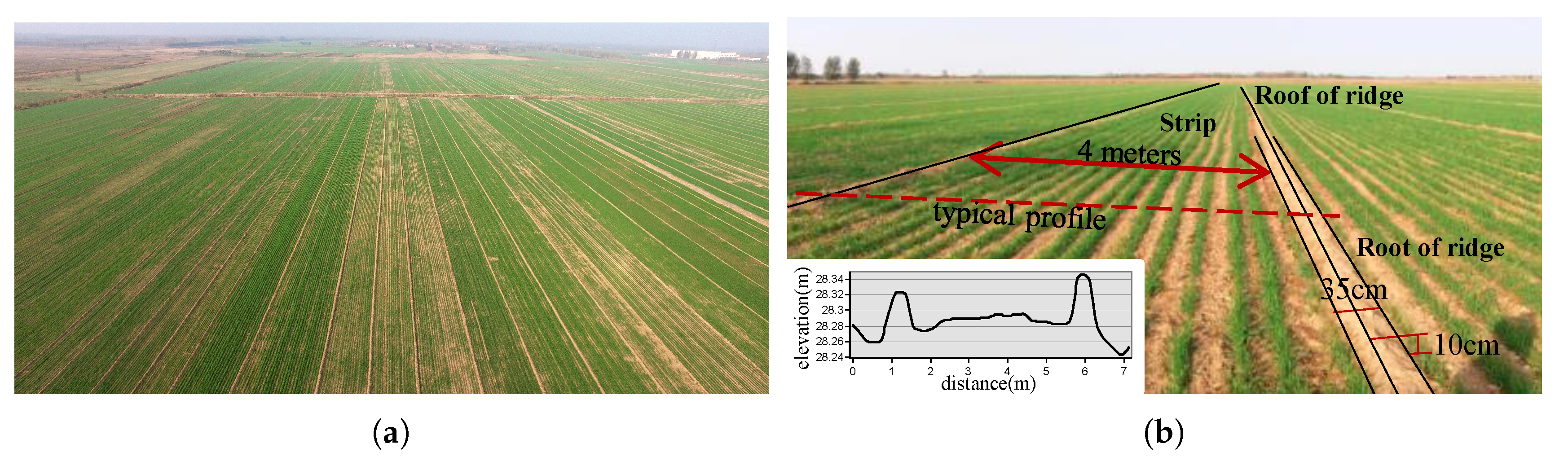
Figure 1.
Typical cropland landscape of (a) aerial view and (b) field photo of actual strips and ridges.
Figure 1.
Typical cropland landscape of (a) aerial view and (b) field photo of actual strips and ridges.
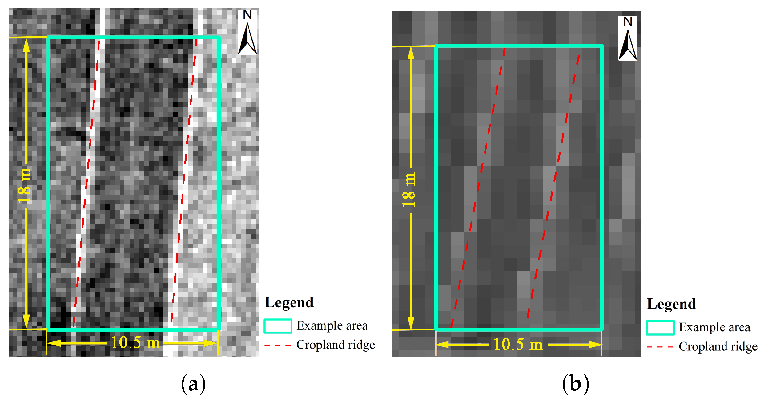
Figure 2.
Limited performance of satellite panchromatic image in cropland ridge identification: (a) WorldView-3 (0.31 m), (b) GF-2 (0.81 m). The bigger the digital number, the brighter the image pixel.
Figure 2.
Limited performance of satellite panchromatic image in cropland ridge identification: (a) WorldView-3 (0.31 m), (b) GF-2 (0.81 m). The bigger the digital number, the brighter the image pixel.
Figure 3.
Pipeline of the methods used in this study.
Figure 3.
Pipeline of the methods used in this study.
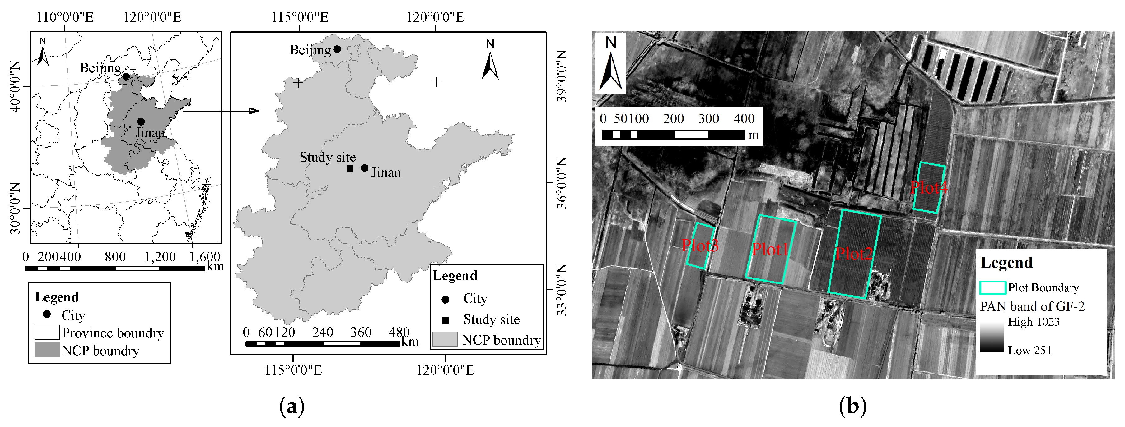
Figure 4.
(a) location of North China Plain (NCP) and study site; (b) location of four plots with a 32-bit panchromatic image from the GF-2 satellite (spatial resolution: 0.83 m) as background.
Figure 4.
(a) location of North China Plain (NCP) and study site; (b) location of four plots with a 32-bit panchromatic image from the GF-2 satellite (spatial resolution: 0.83 m) as background.
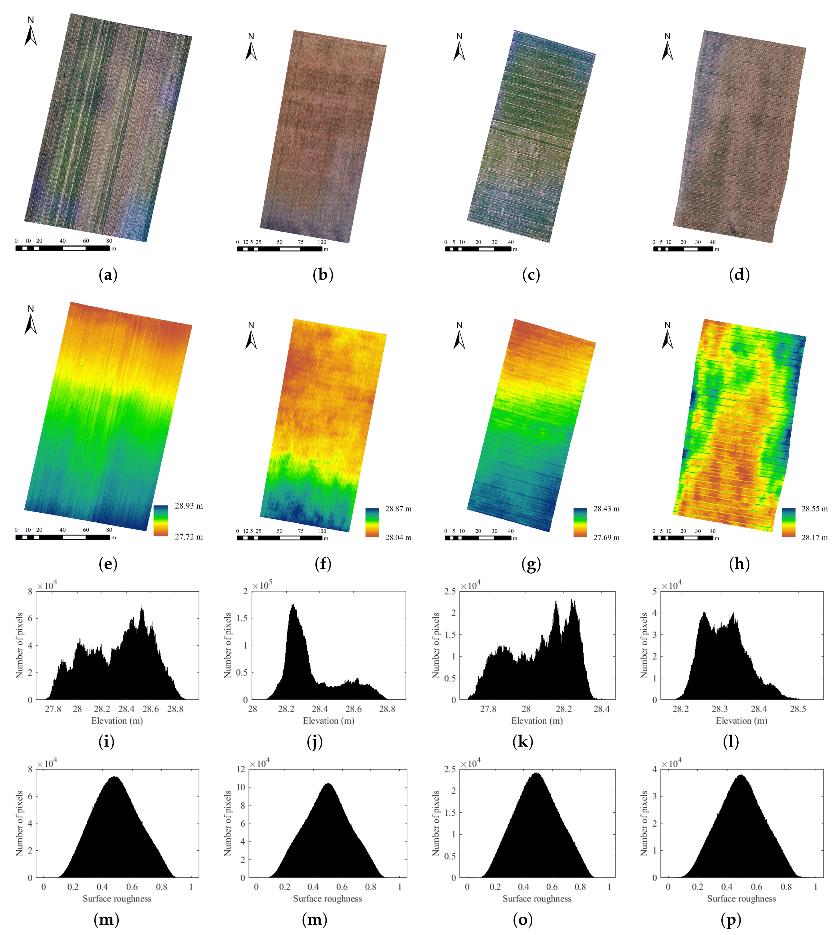
Figure 5.
Plot images of orthophoto for Plot 1 (a), Plot 2 (b), Plot 3 (c), Plot 4 (d), DSM for Plot 1 (e), Plot 2 (f), Plot 3 (g), Plot 4 (h), elevation histogram for Plot 1 (i), Plot 2 (j), Plot 3 (k), Plot 4 (l), and surface roughness histogram for Plot 1 (m), Plot 2 (n), Plot 3 (o), Plot 4 (p).
Figure 5.
Plot images of orthophoto for Plot 1 (a), Plot 2 (b), Plot 3 (c), Plot 4 (d), DSM for Plot 1 (e), Plot 2 (f), Plot 3 (g), Plot 4 (h), elevation histogram for Plot 1 (i), Plot 2 (j), Plot 3 (k), Plot 4 (l), and surface roughness histogram for Plot 1 (m), Plot 2 (n), Plot 3 (o), Plot 4 (p).
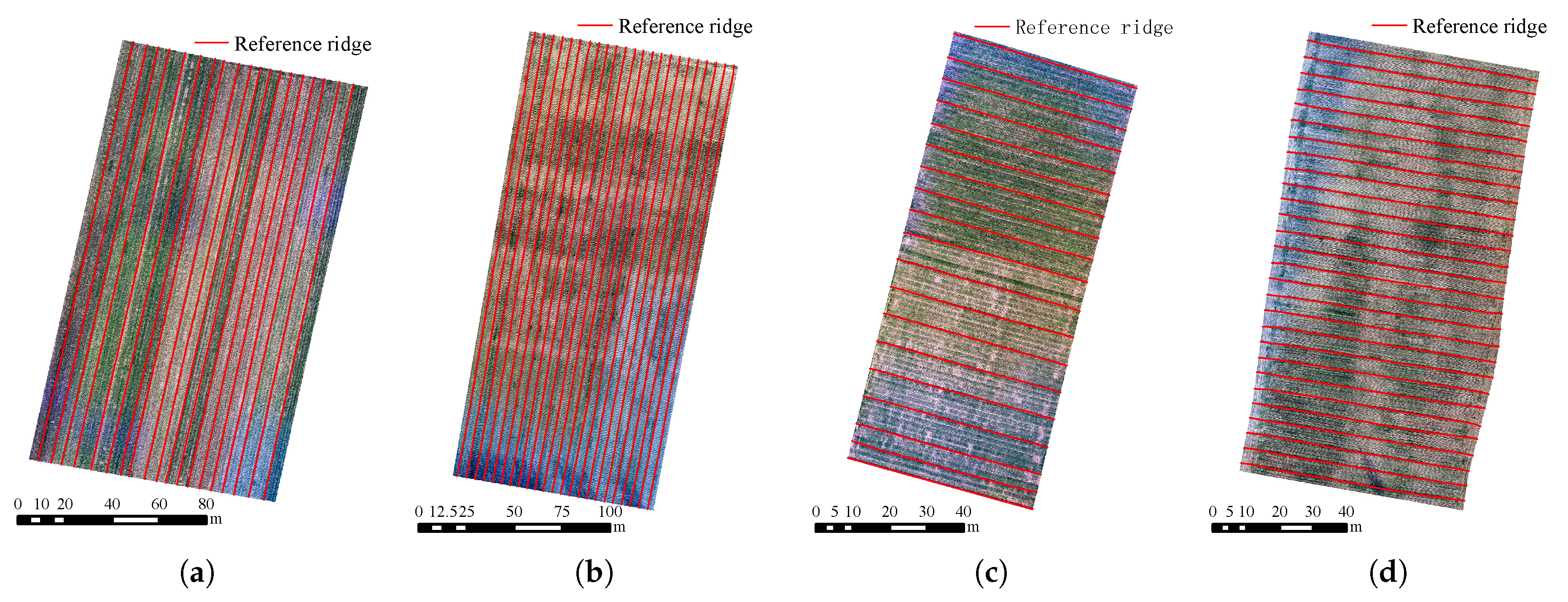
Figure 6.
Validation ridges obtained by manual digitization for Plot 1 (a), Plot 2 (b), Plot 3 (c), Plot 4 (d).
Figure 6.
Validation ridges obtained by manual digitization for Plot 1 (a), Plot 2 (b), Plot 3 (c), Plot 4 (d).
Figure 7.
Typical profile of DSM after processing sUAS images and field photo of actual strips and ridges. (a) typical DSM data and example profile line; (b) typical orthophoto data and example profile line; (c) typical DSM profile with black circles marking ridge peaks.
Figure 7.
Typical profile of DSM after processing sUAS images and field photo of actual strips and ridges. (a) typical DSM data and example profile line; (b) typical orthophoto data and example profile line; (c) typical DSM profile with black circles marking ridge peaks.
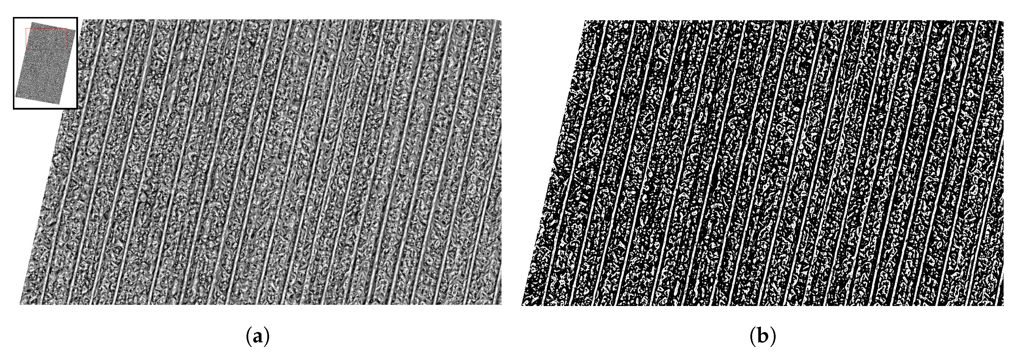
Figure 8.
Binary image before (
a) and after (
b) threshold segmentation. Partial location is displayed in the left upper corner in
Figure 8a. Ridge candidates are valued as 1 in white and non-ridge candidates are valued as 0 in black.
Figure 8.
Binary image before (
a) and after (
b) threshold segmentation. Partial location is displayed in the left upper corner in
Figure 8a. Ridge candidates are valued as 1 in white and non-ridge candidates are valued as 0 in black.
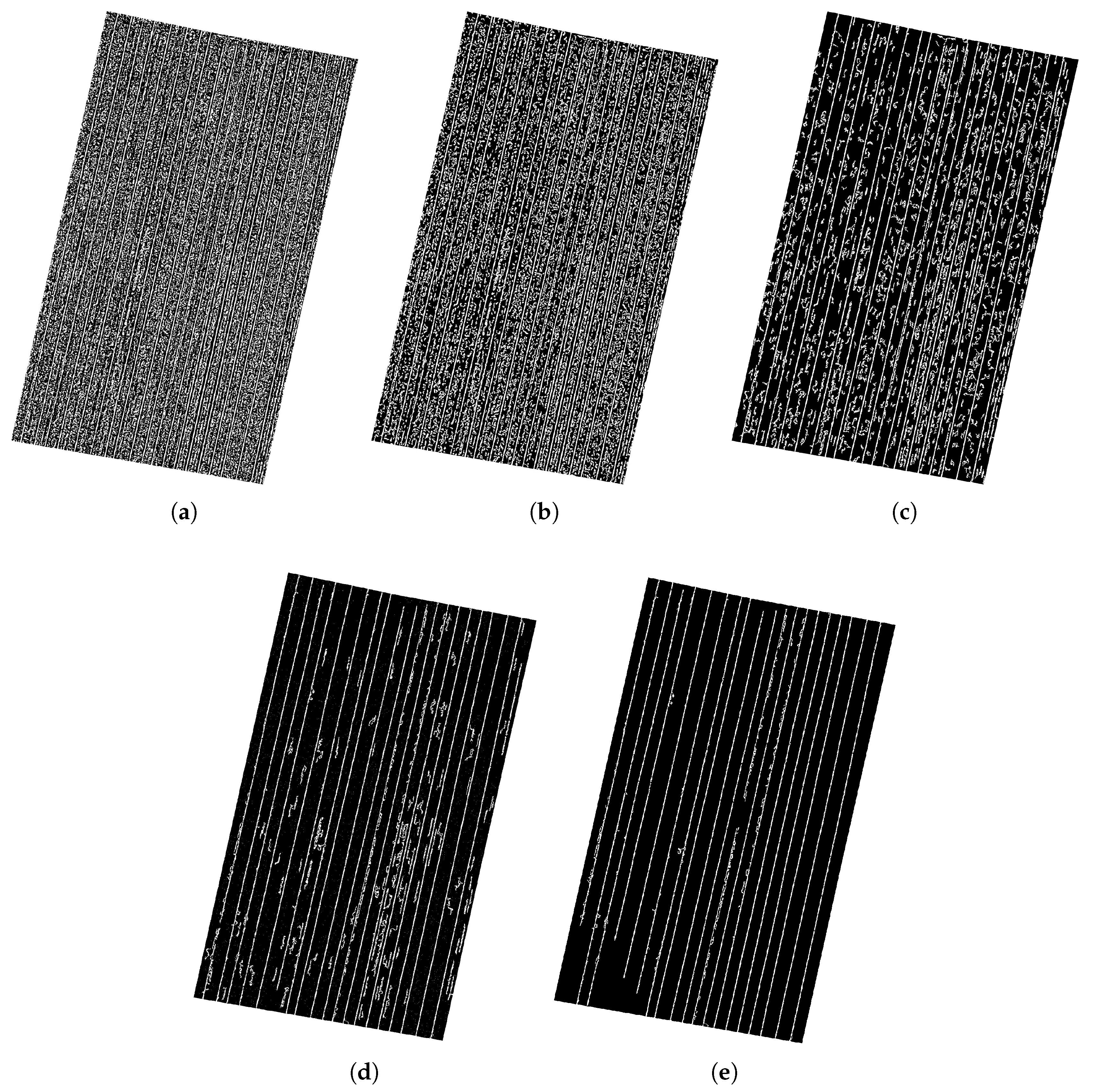
Figure 9.
Extracted results using the shape index filter. Ridge candidates are valued as 1 in white and non-ridge candidates are valued as 0 in black. (a) binary image () as segmented from surface roughness of Plot 1, (b) result () after the first filtering using mean area of , (c) result () after the second filtering using mean MER perimeter of , (d) result () after the third filtering using mean major axis length of , (e) result () after the fourth filtering using MER area of .
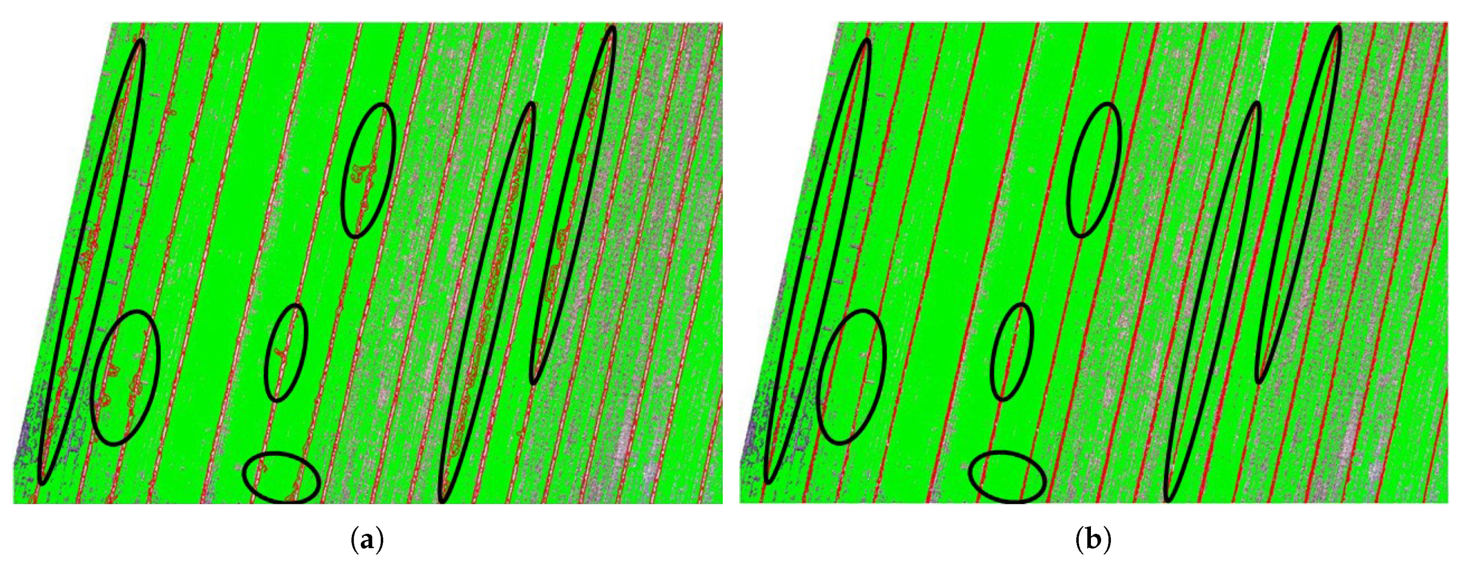
Figure 10.
Ridge extraction before (a) and after (b) removing vegetation impacts in partial Plot 1. Overlaying images are the ridge candidates (red lines) and vegetation coverage (green). Significantly improved ridges are marked with black ellipses.
Figure 10.
Ridge extraction before (a) and after (b) removing vegetation impacts in partial Plot 1. Overlaying images are the ridge candidates (red lines) and vegetation coverage (green). Significantly improved ridges are marked with black ellipses.
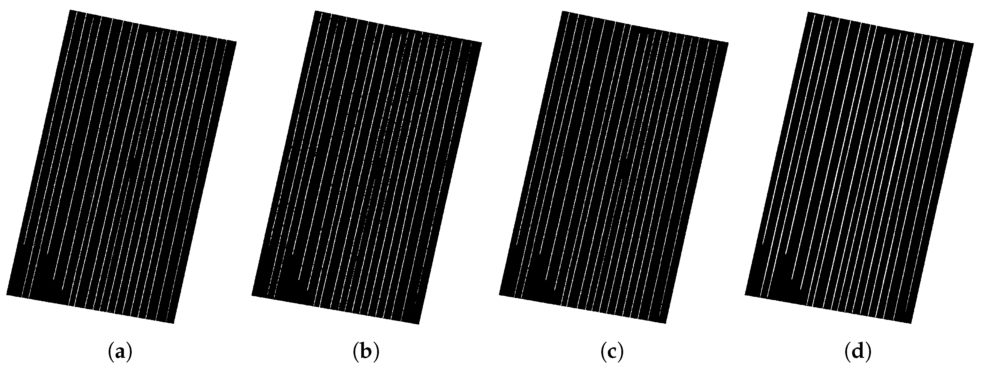
Figure 11.
Final results using morphological operation. Ridge candidates are valued as 1 in white and non-ridge candidates are valued as 0 in black. (a) binary image () after removing vegetation coverage of Plot 1, (b) result () using image opening with MDSE, (c) result () after removing small regions with threshold: 1000 pixels, (d) result () using image closing with SEL.
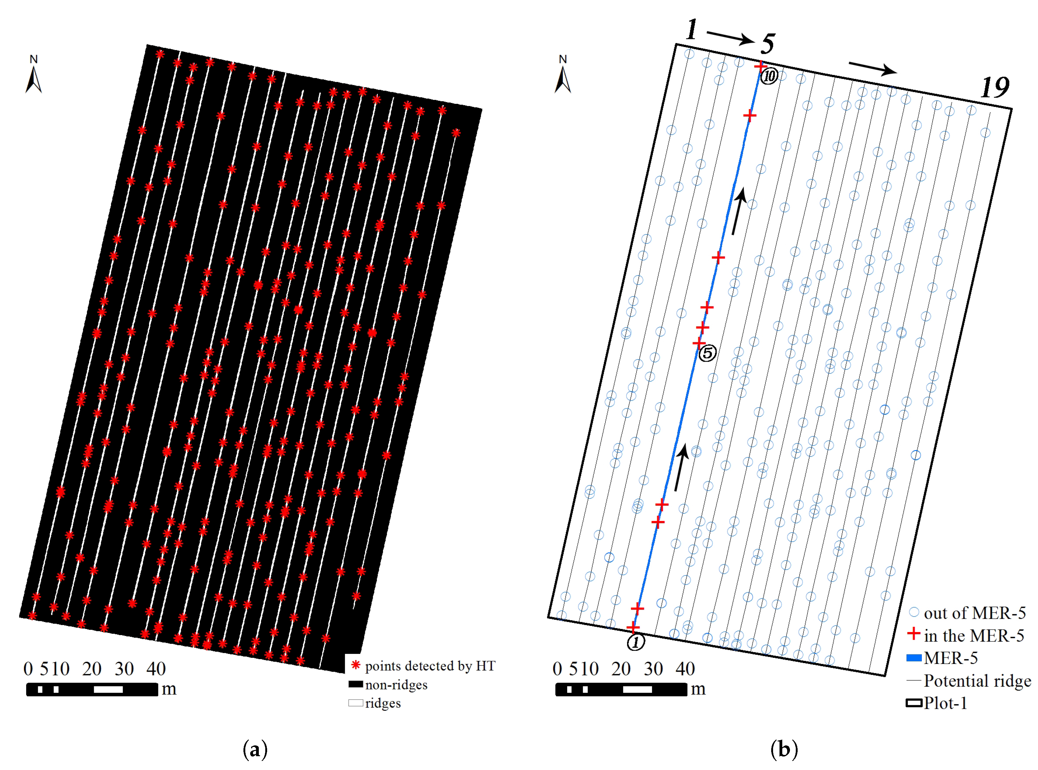
Figure 12.
Point detection using the Hough Transform and point labeling and sorting. The binary image of the ridge candidates is the background. (a) result of point detection using Hough Transform for Plot 1; (b) point labeling and sorting.
Figure 12.
Point detection using the Hough Transform and point labeling and sorting. The binary image of the ridge candidates is the background. (a) result of point detection using Hough Transform for Plot 1; (b) point labeling and sorting.
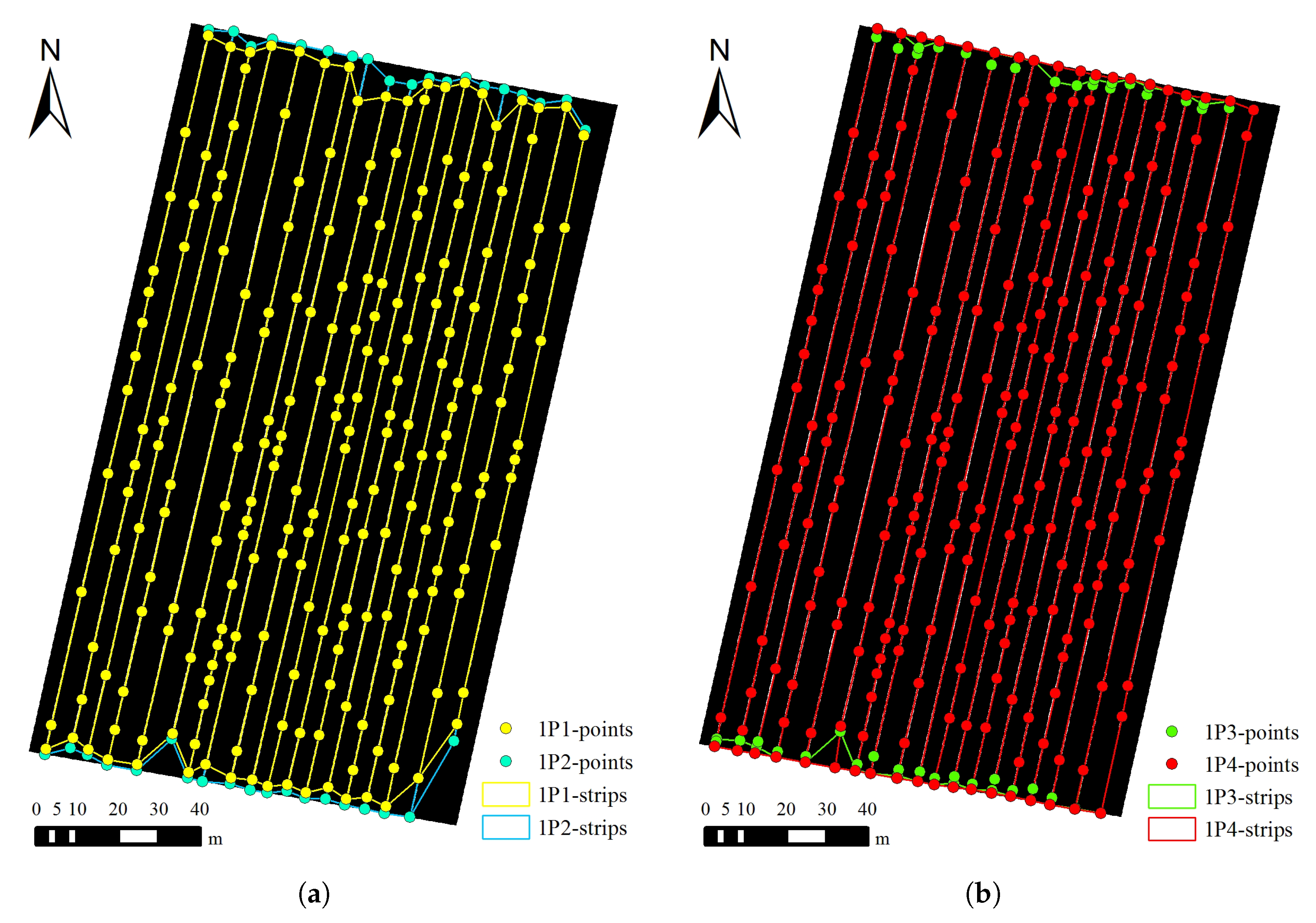
Figure 13.
Results of four steps after point reduction and improvement for Plot 1. The binary image of ridge candidates is the background. (a) overlaying results of point reduction (P1) and comparison with central points of MER minor axis borders (P2); (b) endpoint improvement for corner parts (P3) and other endpoints (P4).
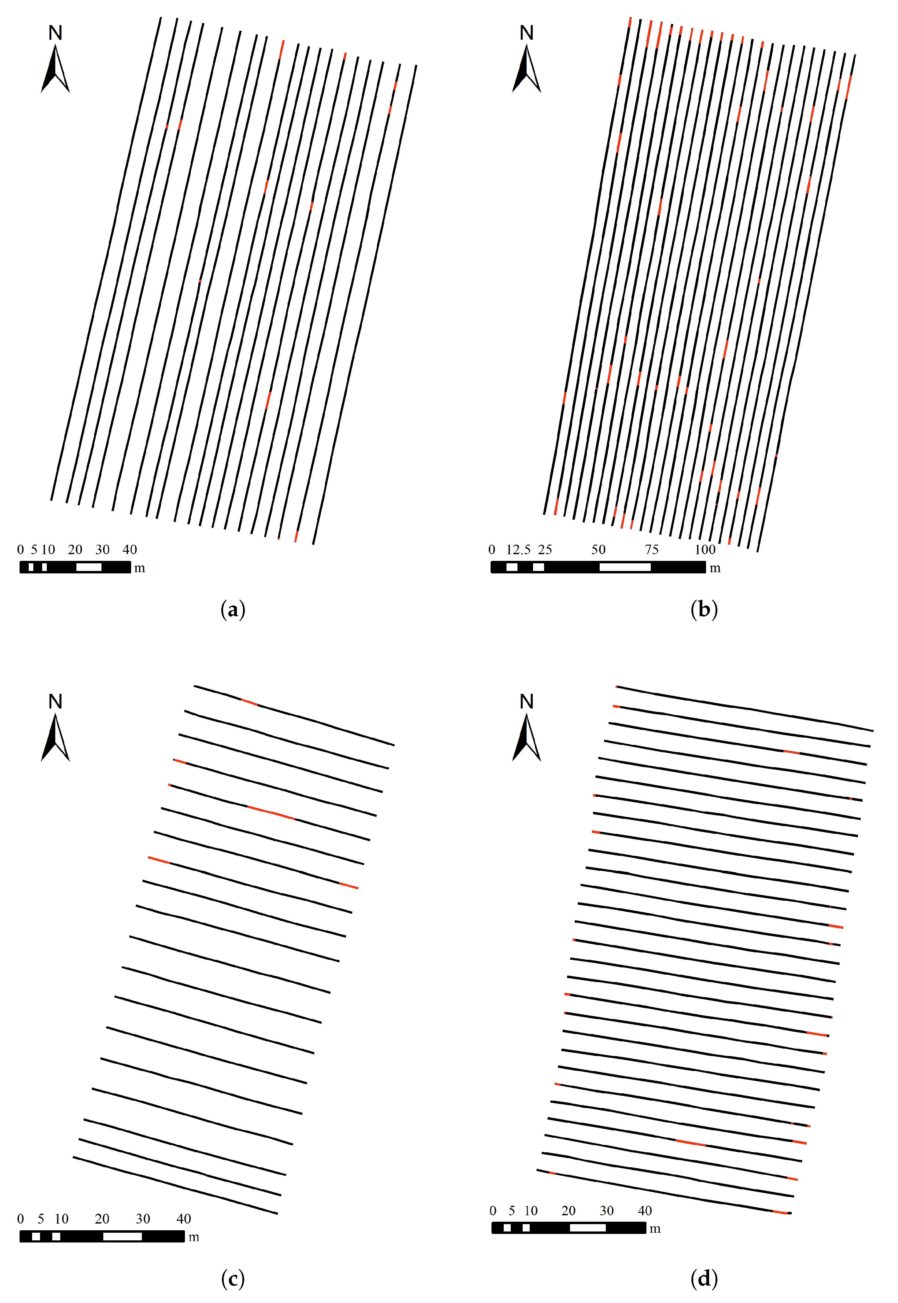
Figure 14.
Ridge detection assessment result. True positives (TP) are black and false positives (FP) are red. (a) Plot 1, (b) Plot 2, (c) Plot 3, (d) Plot 4.
Figure 14.
Ridge detection assessment result. True positives (TP) are black and false positives (FP) are red. (a) Plot 1, (b) Plot 2, (c) Plot 3, (d) Plot 4.
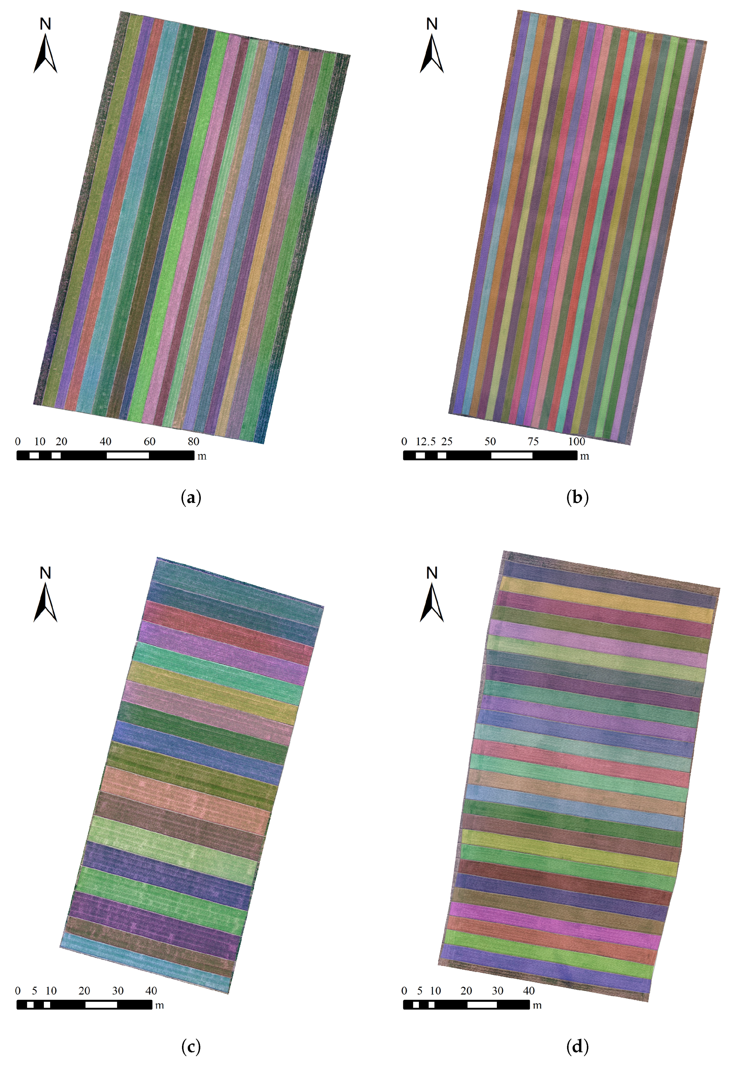
Figure 15.
Extracted strips of four plots filled with different colors. (a) Plot 1, (b) Plot 2, (c) Plot 3, (d) Plot 4.
Figure 15.
Extracted strips of four plots filled with different colors. (a) Plot 1, (b) Plot 2, (c) Plot 3, (d) Plot 4.
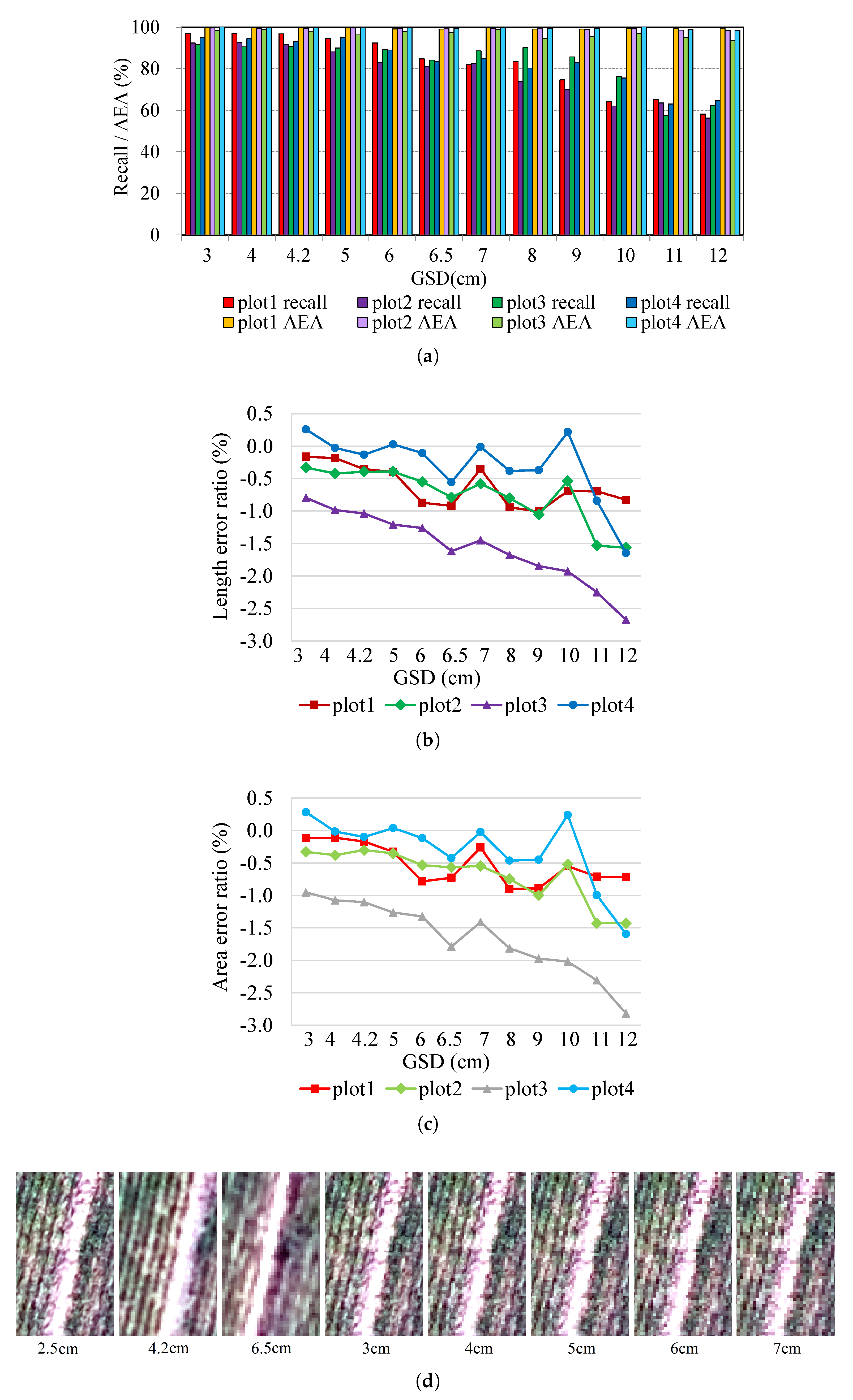
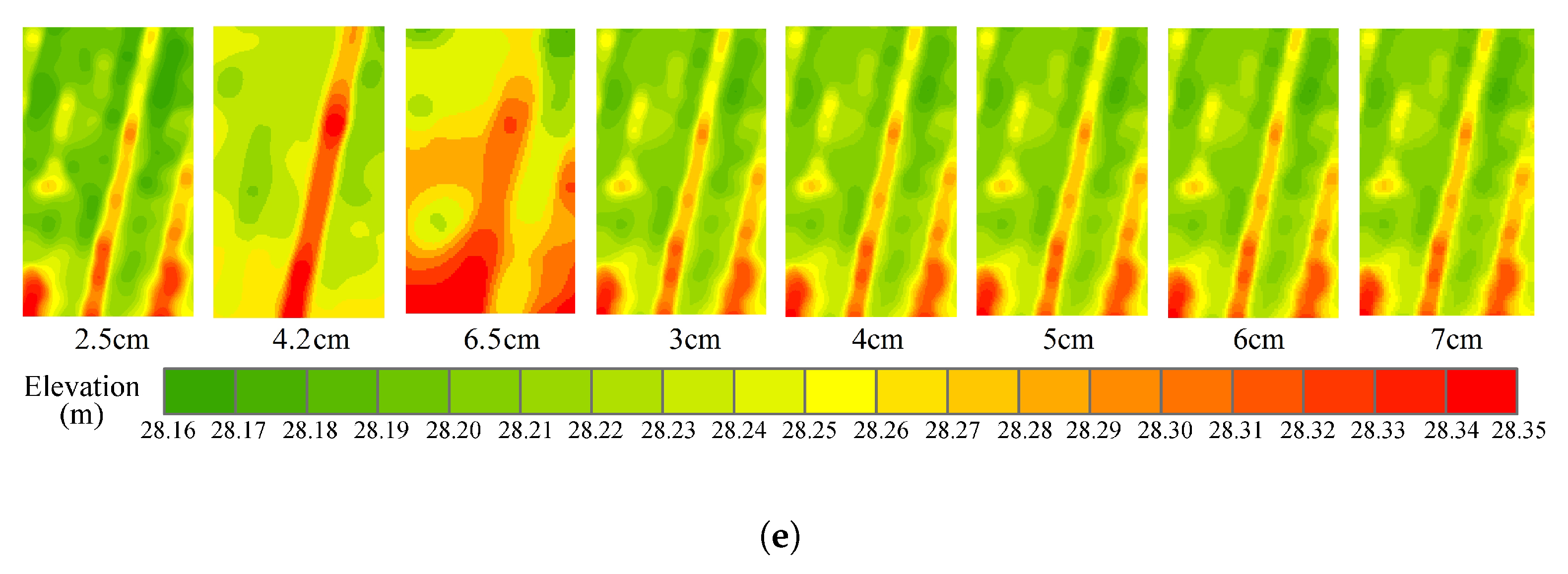
Figure 16.
The impacts on mapping performance of different resolution images: (a) recall and AEA, (b) length ratio error, (c) area ratio error; typical images of cropland ridge: (d) orthophoto and (e) DSM in different GSD with the actual extent: 2.1 m × 3.5 m.
Figure 16.
The impacts on mapping performance of different resolution images: (a) recall and AEA, (b) length ratio error, (c) area ratio error; typical images of cropland ridge: (d) orthophoto and (e) DSM in different GSD with the actual extent: 2.1 m × 3.5 m.
Table 1.
Specifications of sUAS employed in this study.
Table 1.
Specifications of sUAS employed in this study.
| No. | UAV Specification | UAV Parameter | Digital Camera Specification | Digital Camera Parameter |
|---|
| 1 | Diagonal wheelbase | 650 mm | Focal length | 3.64 mm |
| 2 | Maximum takeoff weight | 3.6 kg | Weight of camera and gimbal | 247 g |
| 3 | Maximum payload | 1.0 kg | Sensor size | mm |
| 4 | Maximum AGL | 500 m | Effective pixels | 12.4 megapixel |
| 5 | Hovering accuracy (P-mode with GPS) | Vertical: 0.5 m, Horizontal: 2.5 m | Diagonal field of view | 94 |
| 6 | Capacity of battery (TB48D) | 5700 mAh | Pixel size | 1.55 m |
| 7 | Hovering time (with TB48D battery) | No payload: 28 min, 500 g payload: 20 min, 1 kg payload: 16 min | Sensor type | complementary metal-oxide-semiconductor (CMOS) |
Table 2.
Summary of the sUAS flight parameters for the study site.
Table 2.
Summary of the sUAS flight parameters for the study site.
| Flight Mission | AGL (m) | Date of Flight | Overlap (Front × Side) | Number of GCPs | Resolution (cm) |
|---|
| Mission 1 | 60 | 1 November 2016 | 80% × 60% | 13 | 2.5 |
| Mission 2 | 100 | 2 November 2016 | 80% × 60% | 13 | 4.2 |
| Mission 3 | 150 | 2 November 2016 | 80% × 60% | 13 | 6.5 |
Table 3.
Specific parameters of four plots.
Table 3.
Specific parameters of four plots.
| Plot | Plot 1 | Plot 2 | Plot 3 | Plot 4 |
|---|
| area (m2) | 17,466 | 24,743 | 6228 | 9447 |
| number of cropland strips | 18 | 22 | 18 | 27 |
| ridge width (m) | 0.33 | 0.41 | 0.36 | 0.39 |
| strip, length × width range (m) | 181.5 × (3.8–7.5) | 237.8 × (4.5–5.3) | 52.1 × (5.5–8.0) | 72.3 × (4.7–5.0) |
| elevation, mean(min-max) (m) | 28.33(27.72–28.93) | 28.35(28.03–28.87) | 28.07(27.69–28.43) | 28.31(28.17–28.55) |
| gradient, mean(min-max) | 2.797(0,39.103) | 2.590(0,35.815) | 2.639(0,28.540) | 2.387(0,35.963) |
| surface roughness, mean(min-max) | 0.490(0,1) | 0.495(0,1) | 0.494(0,1) | 0.495(0,1) |
| crop coverage condition | partly | scarcely | partly | scarcely |
Table 4.
Details of pixel shape indexes (PSIs).
Table 4.
Details of pixel shape indexes (PSIs).
| Name | Unit | Concept |
|---|
| Area | pixel2 | Actual number of pixels in the region |
| Area of MER | pixel2 | Area of smallest rectangle containing the region |
| Perimeter of MER | pixel | Perimeter of smallest
rectangle containing the region |
| Major axis length | pixel | Length of the major axis of the ellipse with the same normalized second central |
| | | moments as the objective region |
| Minor axis length | pixel | Length of the minor axis of the ellipse with the same normalized second central |
| | | moments as the objective region |
| Orientation | degree | Angle between the x-axis and the major axis of the ellipse that has the same |
| | | second-moments as the region |
Table 5.
Parameter summary of cropland ridge detection.
Table 5.
Parameter summary of cropland ridge detection.
Table 6.
Accuracy assessment of point reduction and improvement.
Table 6.
Accuracy assessment of point reduction and improvement.
| Plot and | Detected | Mean Length of Ridges | Recall | Total Area of Strips | AEA |
|---|
| Step | Points | (m) | (%) | (m2) | (%) |
|---|
| 1P0 | 286 | 172.7 | 94.1 | 16,658 | 95.4 |
| 1P1 | 223 | 172.4 | 94.4 | 16,634 | 95.2 |
| 1P2 | 261 | 177.8 | 97.3 | 17,161 | 98.3 |
| 1P3 | 261 | 179.3 | 98.1 | 17,250 | 98.8 |
| 1P4 | 232 | 181.2 | 98.6 | 17,439 | 99.9 |
| 2P0 | 275 | 224.7 | 92.4 | 23,447 | 94.8 |
| 2P1 | 246 | 224.7 | 92.4 | 23,439 | 94.7 |
| 2P2 | 290 | 235.2 | 96.5 | 24,475 | 98.9 |
| 2P3 | 290 | 235.1 | 96.5 | 24,472 | 98.9 |
| 2P4 | 262 | 236.6 | 96.8 | 24,626 | 99.5 |
| 3P0 | 296 | 47.1 | 88.9 | 5565 | 90.2 |
| 3P1 | 92 | 39.9 | 76.2 | 4685 | 75.9 |
| 3P2 | 130 | 49.5 | 94.7 | 5889 | 95.5 |
| 3P3 | 130 | 49.8 | 95.4 | 5913 | 95.8 |
| 3P4 | 105 | 51.5 | 97.4 | 6106 | 99.0 |
| 4P0 | 292 | 64.7 | 91.5 | 8354 | 92.0 |
| 4P1 | 208 | 62.0 | 88.0 | 8031 | 88.5 |
| 4P2 | 264 | 67.6 | 95.3 | 8731 | 96.2 |
| 4P3 | 264 | 67.9 | 95.6 | 8748 | 96.4 |
| 4P4 | 222 | 69.6 | 97.1 | 8975 | 98.9 |
Table 7.
Accuracy assessment of ridge detection.
Table 7.
Accuracy assessment of ridge detection.
| Plot | Average Extracted | Average Actual | Length Error | Length Error | Recall | Precision |
|---|
| | Length (m) | Length (m) | (m) | Ratio (%) | (%) | (%) |
|---|
| 1 | 181.2 | 181.5 | −0.30 | −0.16 | 98.6 | 98.8 |
| 2 | 236.6 | 237.8 | −1.24 | −0.52 | 96.8 | 95.4 |
| 3 | 51.5 | 52.0 | −0.49 | −0.94 | 97.9 | 96.9 |
| 4 | 69.4 | 70.3 | −0.95 | −1.35 | 97.1 | 97.5 |
Table 8.
Accuracy assessment of strip extraction.
Table 8.
Accuracy assessment of strip extraction.
| Plot | Automated Extracted | Total Reference | Total Area | Total Area | KC Range |
|---|
| | Area (m2) | Area (m2) | Error (m2) | Extraction Ratio (%) | (%) |
|---|
| 1 | 17,439 | 17,466 | −26.9 | 99.9 | 97.6–99.4 |
| 2 | 24,626 | 24,743 | −117.3 | 99.5 | 97.4–99.3 |
| 3 | 6106 | 6170 | −63.8 | 99.0 | 98.6–99.8 |
| 4 | 8975 | 9075 | −99.6 | 98.9 | 98.5–99.9 |


 ,
, 


