Recent Surface Deformation in the Tianjin Area Revealed by Sentinel-1A Data

Abstract

In this study, we employed multitemporal InSAR (Interferometric Synthetic Aperture Radar) (MT-InSAR) to detect spatial and temporal ground deformations over the whole Tianjin region in the North China Plain area. Twenty-five ascending Sentinel-1A terrain observation by progressive scans (TOPS) synthetic aperture radar (SAR) scenes covering this area, acquired from 9 January 2016 to 8 June 2017, were processed using InSAR time series analysis. The deformation results derived from Sentinel-1A MT-InSAR were validated with continuously operating reference stations (CORS) at four sites and four stations of the Crustal Movement Observation Network of China (CMONOC). The overall results show good agreement, demonstrating the suitability of applying Doris with Sentinel-1A data to high-resolution monitoring of surface deformation. Significant deformation variations have been observed in different parts of Tianjin. These gradually increased from the central part of the metropolitan area to the nearby suburbs. The deformation rate of the main urban area is well-balanced and it is also relatively linear, with uplifting rates ranging from 0 to 20 mm/yr. However, due to the diversity of the geological conditions and anthropogenic activities, remarkable signs of subsidence were found in several parts of Tianjin. In particular, the south-western part of Wuqing District and western part of Beichen District showed subsidence rates of up to −136 mm/yr. We also found that, in addition to groundwater over-exploitation and lithological characteristics, additional factors also influence ground subsidence, including dynamic loads (e.g., railways), static loads (e.g., urban construction), and groundwater recharging.

1. Introduction

Ground subsidence has always been one of the most severe and widespread geological hazards in the cities of China [1]. Over 70,000 km${}^2$ in 17 provinces in China have been directly affected by subsidence [2,3]. The potential consequences of land subsidence mainly include degradation of the aquifer systems and damage to the utility infrastructure, buildings, railroads, highways, and bridges [4]. In 2010, Herrera et al. [5] selected the TerraSAR-X data acquired from July 2008 to September 2009 to study the deformation of the city of Murcia. Detailed discussions were given with respect to the main factors that control the subsidence mechanisms: the thickness of the compressible layer, the presence of pumping wells, and the water table variation. Local analysis of several buildings and infrastructures was presented. The results demonstrated that surface deformation variations were correlated with seasonal variations of groundwater table level. The rapid response of ground deformation to pore pressure changes is explained by the drainage capacity of the aquifer system, and particularly by the presence of sandy layers in shallow acquifers, that increase its permeability. Differential subsidence is caused when different types of foundations of buildings and infrastructures are jointed. With the rapid development of the economy, the amount of groundwater exploitation in cities has also risen sharply. As a result, a series of problems related to urban land surface subsidence have arisen. Surface subsidence is a slowly changing geological hazard that can cause a series of secondary chain of processes that are closely related to important factors such as human production, economic development, and urban development [6]. The North China Plain (NCP), Yangtze River Delta region and the Fenwei basin in China are the three major areas in which serious surface subsidence has occurred over the past few decades. The NCP includes three subsidence centres, in Tianjin, Cangzhou and the north-eastern corner of Beijing. The land subsidence in Tianjin began in the 1920s, accompanying large-scale urbanization and industrialization in Tianjin. After 1949, land subsidence in Tianjin accelerated and the maximum value exceeded $3.1$ m by 2005. This made it the most serious area of subsidence in China [1]. As one of the most serious affected areas in Tianjin, the special location of Wangqingtuo Town cannot be uniformly managed in administrative divisions [7].

To control the rate of land subsidence and reduce its harmfulness effectively, subsidence monitoring is extremely important. This is also basic work that is indispensable for studying the mechanism and trend of development of land subsidence. Traditional methods of land subsidence measurement include levelling, bedrock measurement and stratified measurement. A bedrock standard is a special monitoring point buried in intact underground bedrock by drilling. It is the marker point from the underground bedrock to the surface and acts as a starting point or elevation control point for leveling (i.e., the reference point for stratified target monitoring). Stratified marks are a special monitoring points buried at different depths of the ground layer by drilling methods according to the nature of the soil layer. With the development of modern surveying and mapping technology, GPS surveying has also become an important method of subsidence monitoring. Although traditional levelling and GPS data are able to provide reliable observations of ground subsidence, they are limited by low spatial sampling density and high cost. It is hard to obtain subsidence information with consistent spatial distribution at large scale [6].

In order to overcome these problems, an advanced remote sensing technique, referred to as differential interferometric synthetic aperture radar (D-InSAR), was introduced as a way to monitor deformation over wide areas with centimetre to millimetre accuracy [8]. Repeat-pass satellite InSAR is potentially a unique tool for low cost, precise generation of digital elevation models (DEM) and broad-coverage surface deformation monitoring [9]. The D-InSAR technique uses two SAR scenes of the same area taken at different times and calculates an interferogram that shows the line-of-sight (LOS) ground-surface displacement (range change) between two time periods [8,10,11]. It has been proven to be an effective remote sensing tool for mapping urban land subsidence and is widely used to monitor surface subsidence, landslides, volcano dynamics, earthquakes, snow changes, etc. [12,13,14,15]. However, D-InSAR is susceptible to atmospheric disturbance, and to temporal and spatial decorrelation. These make it difficult to use for long time-interval surface monitoring with high precision [16,17,18]. Temporal decorrelation makes D-InSAR measurements unfeasible over vegetated areas and where the electromagnetic profiles and/or positions of the scatterers change with time within the resolution cell. Geometric decorrelation limits the number of image pairs suitable for interferometric applications and prevents full exploitation of the data sets available. Atmospheric inhomogeneities create an atmospheric phase screen (APS) superimposed on each SAR image that can seriously compromise accurate deformation monitoring [18].

In summary, under the influence of decorrelation factors and atmospheric delay effects, the accuracy in deformation monitoring achieved with the traditional D-InSAR method is generally not high enough, ranging from the decimetre to centimetre level. However, the accuracy of deformation monitoring often needs to be higher, so D-InSAR has substantial limitations in urban infrastructure monitoring applications. To overcome temporal and spatial decorrelation and the atmospheric delay of D-InSAR and to improve the applicability of the D-InSAR technique, multi-temporal InSAR (MT-InSAR) was developed to extract and analyse high precision and high density measurement points using multi-view SAR images. In 2001, Ferretti et al. [9] proposed a kind of MT-InSAR, the ‘permanent scatterers’ InSAR (PS-InSAR) method—known as the first persistent scatterers interferometry (PSI) technique [19,20]—a powerful technique for wide-area deformation monitoring with millimetre accuracy [21]. Reliable deformation and height correction information can be obtained by adopting stable scattering targets (buildings, structures, etc.) from a long temporal series of interferometric stacks. Later, Berardino et al. [22] proposed a small baseline subset InSAR (SBAS-InSAR) method to study low-resolution, large-scale deformation. SBAS-InSAR is another TS-InSAR method that effectively mitigates decorrelation phenomena by analysing distributed scatterers (DSs) with high coherence based on an appropriate combination of interferograms. These can reduce the geometrical and temporal decorrelation more than with PS-InSAR [22,23,24].

There has been some debate about the relative merits of the PS and SBAS methods. However, because they are optimized for different models of ground scattering, the two approaches are in fact complementary, at least in the usual case where a data set contains pixels with a range of scattering characteristics; the scattering characteristics of the terrain are often between these two models. Recently, both of these two advanced InSAR techniques have been widely used in monitoring urban ground deformation around the world. For instance, Perissin and Wang [25] used PS-InSAR to monitor subsidence and landslides in urban areas of China (e.g., Shanghai, Tianjin, and Badong) and near the Three Gorges Dam. Heleno et al. [26] used PS-InSAR to detect and measure ground subsidence in Lisbon, Portugal. Castellazzi et al. [27] applied the SBAS-InSAR method to monitor the spatiotemporal variations of displacements and fracturing from 2012 to 2014 in Mexico. Bai et al. [4] presented results based on SBAS-InSAR observations to monitor the ground deformation in the Wuhan region of China.

In 2008, Hooper et al. [28] presented a new algorithm (released software package ‘StaMPS/MTI’ (Stanford Method for Persistent Scatterer/Multi temporal InSAR)) that combined both the PS and SBAS approaches to maximize the spatial sampling of a useble signal and get a higher signal-to-noise ratio than with either approach alone. Improvement of the spatial sampling is important, not only because the resolution of any deformation signal is increased, but it also enables more reliable estimation of integer phase-cycle ambiguities present in the data (phase unwrapping).

Over the past few decades, several techniques based on InSAR have proven an effective way to detect ground deformation related to several dynamic process, such as earthquakes [29], permafrost degradation [30], volcanic eruptions [31], groundwater induced subsidence [5,32,33,34,35], building monitoring [36], landslide activity [37], and especially for land subsidence [38,39,40,41,42,43,44]. Bianchini et al. [37] also presented a review on different applications of persistent scatterers InSAR approaches, proposed and applied over the Tuscany region, Italy across time. With the application of ERS-1/2 to Sentinel-1 data, Solari et al. [43] derived 25 years of land subsidence in Italy; the relationship between the occurrence of the displacement and its main driving factors were also discussed.

In this paper, we present the first investigation of land deformation in the Tianjin area based on the Sentinel-1A terrain observation by progressive scans (TOPS) data with Delft object-oriented radar interferometric software (Doris ) at large scale. The StaMPS approach was applied to 24 ascending Sentinel-1A scenes acquired from 9 January 2016 to 8 June 2017 to retrieve and characterize spatiotemporal variations of ground deformation in the Tianjin region. Moreover, the corresponding validation, detailed illustration, and analysis provided were done using the results of the MT-InSAR and GPS time series. Finally, the potential factors influencing subsidence and analysis of the mechanisms were investigated from the viewpoint of geological tectonic movement, urban development and various external factors.

2. Study Area and Datasets

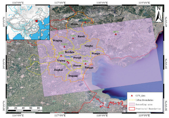
2.1. Study Area

Tianjin is located at the junction of three tectonic units, with the east-west trending Yanshan mountain structural high to the north, the north-easterly Taihang mountain structural high to the southwest and the North China rift-depression basin to the south and southeast. The city is also on the western shore of the Bohai Gulf [45]. Tianjin is separated by the Baodi-Ninghe Fault into two parts, with the northern part on the Yanshan Folded Belt. The southern part is in the Bohai Bay Basin, which contains three tectonic divisions: the Jizhong Depression, Cangxian Uplift, and Huanghua Depression. The Jizhong Depression and Cangxian Uplift are separated by a Paleogene lacuna. The Cangxian Uplift and Huanghua Depression are separated by the Cangdong Fault [46]. To control further deterioration of the land subsidence condition in Tianjin, during 1995, a special group named the ‘Tianjin Office of Land Subsidence’ was set up. To date, 2100 benchmarks (BMs), 2 bedrock marks, 14 layerwise marks, 503 groundwater monitoring wells, 11 continuously operating reference stations (CORS), and 35 GPS stations have been built to monitor land subsidence [47,48].

The study area of our research covers almost all districts, except for a few small parts of Tianjin. The overall study area was approximately 170 by 167 km (Figure 1). It covered Ninehe and Jinghai Counties, Jixian, Baodi, Wuqing, Beichen, Dongli, Jinnan, and Binhai new districts (i.e., Hangu, Tanggu, and Dagang). Figure 2 illustrates the tectonic framework of the study area.

2.2. Sentinel1-A Datasets

In order to investigate the latest land deformation over the whole of Tianjin, 25 ascending Sentinel-1A TOPS SAR scenes with VV polarisation from the European Space Agency (ESA) were processed. As we considered only the ascending orbit dataset, negative values could only show subsidence in flat plain sectors; this was not valid for hilly and mountainous sectors, where the geometry (slope and aspect) of the mountain and hill sides influences the LOS velocity values. Except for a small part in the northeastern corner which is mountainous area, the study area is a flat plain. Therefore, the deformation results are reliable in the area we discuss below. Data were acquired from 9 January 2016 to 8 June 2017. The Sentinel-1A TOPS mode data consist of series of bursts with mutual overlaps, which provides a wide swath with resolution of 5 × 20 m [49]. To improve the solution efficiency, swath1 and swath2 were selected for each of the scenes. Detailed parameters of the Sentinel-1A data are given in

Table 1. Parameters of the Sentinel-1A data.

Parameters	Description
Orbit direction	Ascending
Product type	SLC (Single Look Complex), IW (Interferometric Wide swath) mode
Path	56
Frame	121
Central incidence angle (degree)	33.7
Azimuth angle (degree)	−13.4
Azimuth resolution (m)	20
Range resolution (m)	5
Polarization	VV
Number of scenes	25
Time range	9 Jan 2016–8 Jun 2017

.

The Shuttle Radar Topography Mission (SRTM) data product released in 2015 by the U.S. Geological Survey (USGS) with a spatial resolution of 1 arc-second (30 m) was used to remove the topographic phase [4,27] (https://lta.cr.usgs.gov/SRTM1Arc). Finally, time series for 2015 to 2018 from four continuously operating reference stations (CORS) and four stations of the Crustal Movement Observation Network of China (CMONOC) were utilised to evaluate the results derived from Sentinel-1A MT-InSAR data.

3. MT-InSAR Data Processing with the Application of StaMPS

In the traditional PS-InSAR technique [9], PS candidates (PSC) are selected based on thresholding pixel amplitude dispersion with time, and a temporal linear deformation model is assumed. For high signal-to-noise ratio (SNR) targets, this PS method and its variant [50,51] have been successfully used for picking bright PS, e.g., urban areas with much man-made construction. Without prior assumptions about its temporal nature, StaMPS takes spatial correlation of phase into consideration and succeeds in picking PSC with low SNR scatterers in the natural terrain [20,49]. The StaMPS software package, which contains the PS, SBAS, and combined MT-InSAR algorithms, can be download from http://www.hi.is/~ahooper/stamps [52]. The general processing procedures used for StaMPS-PS are briefly introduced in the following steps; a more detailed description can be found in [20,28,52].

3.1. Interferogram Formation

Firstly, Doris software was used to generate the interferograms needed [53,54]. Generally, at least 25 interferograms are required based on the functional temporal model [28,55]. However, according to Hooper et al. [28], if StaMPS is applied, the number of the required interferograms can be reduced to approximately 12. In this study, 25 scenes were applied to generate the interferograms (Figure 3). In order to minimize the temporal and spatial decorrelation, the scene acquired on 22 December 2016 was selected as the master image, and all of the remaining scenes were co-registered and resampled in relation to the master image. Next, the topographic phase was removed from the interferograms using the SRTM data.

3.2. PS Pixel Selection

Next, PS methods of the StaMPS software package have been used to process the images [20,28,46]. Initially, StaMPS selected a subset of pixels that included almost all of the PS pixels based on an analysis of their amplitude dispersion. The amplitude dispersion index, $D_A$, was defined by [9] as:

$$D_A=\frac{{\sigma }_A}{{\mu }_A},$$

(1)

where ${\sigma }_A$ is the standard deviation and ${\mu }_A$ is the mean of a series of amplitude values. Generally, a threshold value of $D_A$ is used to select PSC. For different study areas, [9,28] adopted threshold values of 0.25 and 0.40, respectively. Because most of the area under investigation was covered by natural vegetation, the threshold value we adopted was 0.40. After selection of a subset of pixels as the initial PSC, StaMPS estimated the phase stability for each of them using phase analysis. The wrapped phase of the x-th point in the i-th interferogram, can be illustrated as follows [9,28,56]:

$${\varphi }_{x,i}={\varphi }_{def,x,i}+{\varphi }_{\alpha ,x,i}+{\varphi }_{orb,x,i}+{\varphi }_{\epsilon ,x,i}+n_{x,i}$$

(2)

where ${\varphi }_{def,x,i}$ is the phase change due to surface deformation of pixels in the direction of LOS, ${\varphi }_{\alpha ,x,i}$ is the phase of atmospheric delay between different passes, ${\varphi }_{orb,x,i}$ is the residual phase caused by satellite orbit error, ${\varphi }_{\epsilon ,x,i}$ is the phase due to look angle error (DEM error), $n_{x,i}$ is noise (e.g., thermal effect, coregistration error, azimuth phase center uncertainty, etc.). Based on the error characteristics of the variables in Equation (2), [28] defined a phase stability indicator ${\gamma }_x$ (3) to evaluate whether the pixel is a PS:

$${\gamma }_x=\frac{1}{N}\left|\sum _{i=1}^{N}exp\left\{\sqrt{-1}\left({\varphi }_{x,i}-{\tilde{\varphi }}_{x,i}-\Delta {\widehat{\varphi }}_{\epsilon ,x,i}^u\right)\right\}\right|$$

(3)

where N is the number of interferograms, ${\tilde{\varphi }}_{x,i}$ is a wrapped estimate of the spatially correlated parts on the right side of Equation (2). ${\widehat{\varphi }}_{\epsilon ,x,i}^u$ is the estimate of the uncorrelated part of ${\varphi }_{\epsilon ,x,i}$. Once this solution has converged to the estimated stability of each pixel and stops iterating, the resulting PS pixels was selected. Typically, PS pixel densities of 5–10 px per km${}^2$ is required to properly estimate and remove atmospheric heterogeneity. With the different threshold values of the amplitude dispersion we selected, each of the PS densities could be raised to 145 px per km${}^2$ by StaMPS.

3.3. Three Dimensional Phase Unwrapping and LOS Deformation Rates Deriving

Phase unwrapping is the process of recovering data from only known modulo 2$\pi$ radians phase to unambiguous phase values. For large displacement of this area, a full three-dimensional (3-D; two spatial dimensions, as with conventional InSAR, and one temporal) unwrapping algorithm is required to derive the deformation rates [57]. Before unwrapping, the spatially uncorrelated term DEM error was subtracted. After unwrapping, there are still four error terms in Equation (2). The spatially correlated portion of these errors are assumed to be temporally uncorrelated. Thus, high-pass filtering the unwrapped data in the temporal dimension and low-pass filtering in the spatial dimensions was applied to estimate the spatially correlated error [57]. Then least-squares inversion was applied to derive the LOS displacement time series for PS points [52], and all the PS points were calibrated to a stable CORS reference station located in the north-east corner of Tianjin (Figure 12).

4. Results and Validation

4.1. Precision Evaluation

At present, there are two methods to assess the accuracy of the PSInSAR technology. One is represented by Politecnico di Milano, which uses the SNR to calculate the noise of the signal [58,59,60]. Another method comes from the Delft University of Technology and establishes the statistical relationship of various phase components. The accuracy of the PS points is finally determined based on the error propagation principle [53,61]. As shown in Equation (3), the PS points were identified based on coherence in the temporal dimension. Therefore, the first method was adopted for accuracy assessment.

For temporally correlated radar targets, noise is mainly caused by the uncorrelated noise of the PS points. Generally, the residual phases are considered to conform to a normal distribution. The relationship between the temporal coherence and the phase variance of PS points can be expressed as: Equation (4):

$$\mathbb{E}\left[\left|\gamma \right|\right]\approx \mathbb{E}\left[{\gamma }_R\right]=e^{-\frac{{\sigma }_{\omega }^2}{2}}$$

(4)

where the standard deviation of the phase ${\sigma }_{\omega }$ can be obtained by the temporal coherence value $\widehat{\gamma }$:

$${\widehat{\sigma }}_{\omega }\approx \sqrt{-2\ln \left|\widehat{\gamma }\right|}$$

(5)

where $\widehat{\gamma }$ is the estimated value of ${\gamma }_x$, which can be obtained from Equation (3). The velocity accuracy of the PS points can be illustrated as

$${\sigma }_v^2\approx \frac{{\sigma }_w^2}{{\left(\frac{4\pi }{\lambda }\right)}^2·{\sum }_{i=1}^N{\left(T_i-\overline{T}\right)}^2}$$

(6)

where $\lambda$ is the C-band microwave wavelength used by the Sentinel satellite. $T_i$ is the i-th acquisition date of the images and $\overline{T}$ is the mean value of $T_i$.

The values mentioned in this section are all ‘precision of inner coincidence’, which are obtained based on the phase stability. This mainly reflects the dispersion of the phase for PS points in the time dimension. The distribution of the calculated temporal coherence $\widehat{\gamma }$ for all of the PS pixels are illustrated in Figure 4 and the values of the statistics are summarized in

Table 2. Statistics table for the calculated temporal coherence.

Phase Correlation	Min	Max	Mean	>0.7
Statistics	0.161	0.999	0.827	81.280%

.

The relationship between the temporal coherence $\widehat{\gamma }$ and the theoretical value of the velocity accuracy for PS points is also given as in Figure 5. In theory, we can find that the accuracy of the velocity ${\sigma }_v$ can reach up to about 2 mm/yr when the coherence reaches 0.7 for each PS point. Although this velocity accuracy is the theoretical limit, it can also explain the reliability of the derived velocity for most of the PS points to some extent.

In order to access the accuracy of the derived velocity, the standard deviation of the velocity for PS points in the direction of LOS have been shown in Figure 6. It shows that the accuracy rate is very high in most areas, except for the southern area and a small part of Tangshan. This was mainly caused by phase unwrapping errors, especially in the edge region where 3-D phase unwrapping could not be well constrained. Results indicate that the minimum, maximum, and mean standard deviation of the derived velocity for PS points are 1.841 mm/yr, 12.124 mm/yr, and 4.761 mm/yr, respectively. Root-mean-square error reached 5.015 mm/yr. For 60.720 % of the PS points, the standard deviation was less than 5 mm/yr, and over 99.31 % of all PS points retain a relatively high precision with the error lower than 10 mm/yr. Furthermore, we also compared the results between the theoretical and calculated statistics of the standard deviation, as shown in Figure 7. For the theoretical value of the standard deviation, most of the PS points range from 0.5 mm/yr to 1.5 mm/yr, while the calculated standard deviations are mostly between 2.5 mm/yr and 4 mm/yr. These inner coincidence results suggest that the deformations derived by InSAR are reliable.

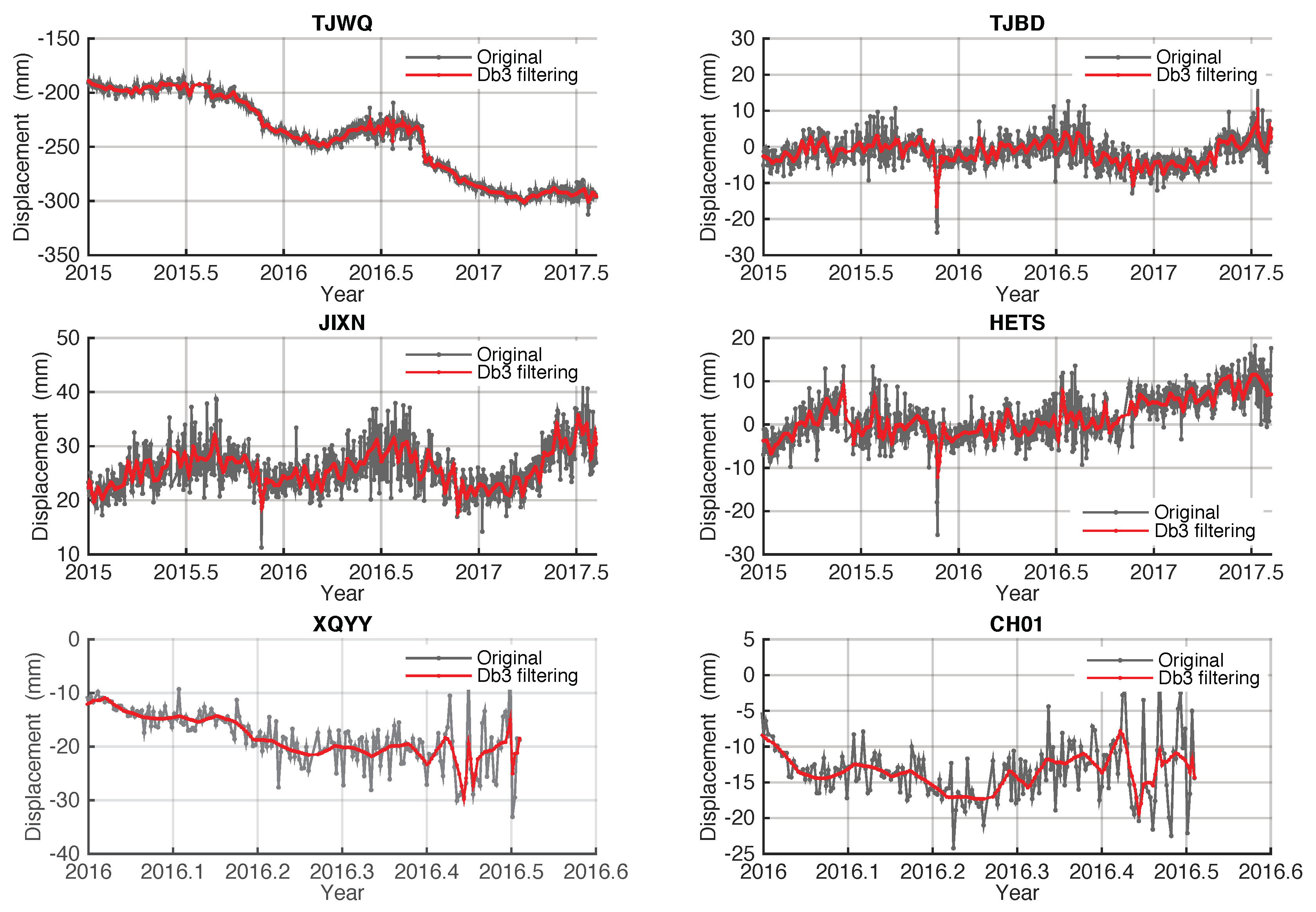
4.2. Validation with GPS Time Series

To further verify the accuracy of the InSAR derived results, a comparative analysis was performed by comparing the results with the GPS time series. Before comparison, all of the GPS time series were projected along the LOS direction and all the PS pixels located within a circle with 50 m radius around the corresponding GPS station were selected. Time series of the two CORS stations (i.e., XQYY and CH01) and the corresponding PS points were all referenced to the JIXN CORS station, as can be seen from Figure 10. This time series is relatively stable and the velocity in the direction of LOS was only 1.9 mm/yr. The other GPS time series were also referenced to a stable IGS (International GPS Service) station. In addition, all of GPS time series and the InSAR results were referenced to the data of the master image (22 December 2016). Due to various random noises in the GPS time series, a Db3 wavelet was introduced to filter the original data [48], as shown in Figure 8 and Figure 9.

The Daubechies extremal phase wavelets (dbN) refers to a particular family of wavelets. N is the order of the wavelet and refers to the number of vanishing moments. Basically, the higher the number of N, the smoother the wavelet (and longer the wavelet filter). A wavelet with N vanishing moments is orthogonal to polynomials of degree at most N. In this paper, the Db3 wavelet was used to filter the original GPS time series.

Figure 9 indicates that the SNR of the time series improved after the filtering was implemented. After the above data processing, we compared the deformation time series of GPS and InSAR, as shown in Figure 10. Since time series of XQYY and CH01 are too short, it is not reliable for us to compare the results with a limited time series. Therefore, these two stations were removed for validation. A curvilinear regression analyzing method was also applied for quantitative assessment the accuracy of PS time series. The results were that root mean square errors for TJWQ, TJBD, JIXN and HETS were 4.35 mm, 4.69 mm, 7.27 mm and 5.03 mm, respectively. Generally, the GPS and InSAR-derived deformation time series may not be consistent with each other. Since there was no Sentinel-1B data in Tianjin area during the investigated time period, there is a long time interval for other scenes, and only Sentinel-1A data was used to derive the deformation velocity, which may have led to three-dimensional phase unwrapping errors. Due to the long time interval of the Sentinel data and the severe subsidence situation in Tianjin, it could lead to poor coherence between scenes and phase unwrapping errors. Furthermore, a linear model was adopted to fit the Sentinel-1A image, which might generate unwrapping errors and lead to misleading results [48]. Despite these issues, the long-term trends for both time series show good consistency. These results suggest that it is reliable enough for further research on the mechanism of deformation in Tianjin.

4.3. Time Series of Deformation

According to the processing procedure mentioned above, the cumulative time series of vertical deformation for Tianjin and its surrounding area were derived, as shown in Figure 11. To obtain a better surface deformation trend in this area, the oldest image, acquired on 9 January 2016, was selected as the time reference.

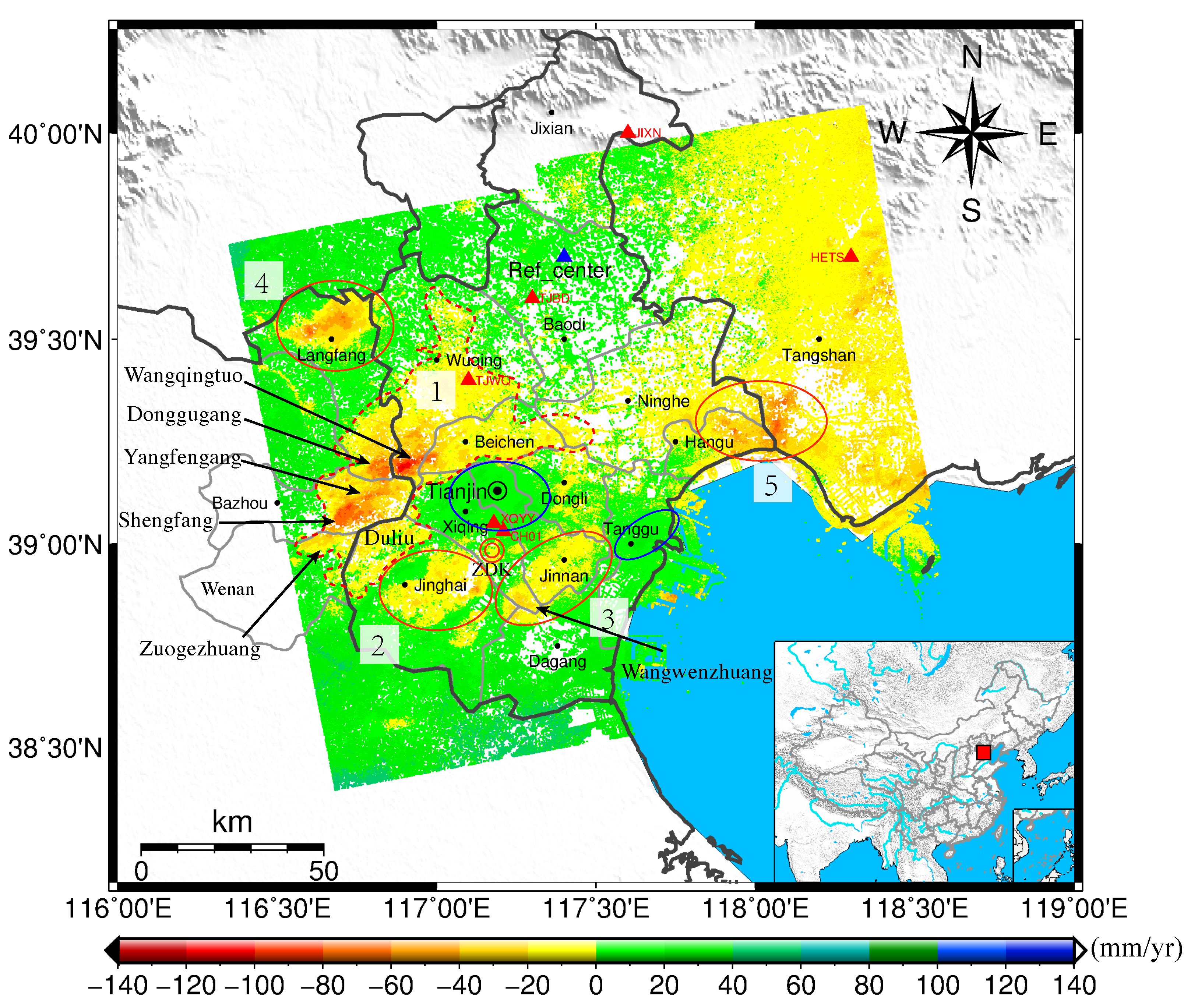
4.4. Mean Velocities Derived from Sentinel-1A Data

Figure 12 shows the annual surface deformation rates derived by the PS technique along the LOS direction of ascending pairs. The blue triangle denotes the reference points (TJA2), located in the north-east of Tianjin, north of Baodi District. The positive and negative signs indicate uplift and subsidence, respectively, in the direction of LOS. A total of approximately four million PS pixels were ultimately identified. Due to the difference in the distribution of man-made objects, significant gaps exist between different parts of Tianjin. The distribution of PS points with higher density are approximately located in the southern part of Wuqing District, the southwest part of Beichen District, in central Tianjin, in central south Dongli District, in north and central Binhai New District, in Jinnan District, and in Jinghai District. Other areas with more vegetation have fewer PS points.

From the spatial distribution of land subsidence, the center of the subsidence area exhibited two large shifts. In the early 1980s, with the completion of the Luanhe-Tianjin water diversion project, subsidence funnels were transferred from the central city to four districts in the vicinity (i.e., Beichen, Dongli, Jinnan, and Xiqing) and to Jinghai District. In recent years, in additional to Jinghai district, with the increasing control of ground subsidence in the four districts, the subsidence funnels have been transferred to Hangu district, and the junction of Wuqing, Beichen and Xiqing districts.

As illustrated in Figure 12, heterogeneous land deformation patterns are widely found in different districts of Tianjin and its surrounding cities. The deformation rates are relatively linear in the north part of Tianjin (i.e., Jixian, north Wuqing, Baodi, and north Ninghe). Actually, this is related to the geological conditions of these areas, where the groundwater is mainly stored in an aquifer with small storage, so that it has not been withdrawn.

The deformation rates in the main urban areas of Tianjin are well-balanced and stable, and exhibit a uplifting trend. The average deformation rate along the direction of LOS reached 7.98 mm/yr, which indicates that the subsidence of Tianjin has been well controlled in recent years. Additionally, we found that the subsidence rate gradually increased from central Tianjin toward the surrounding areas. These subsidence areas include mainly three parts (Region 1 to 3 in Figure 12 ).

Among these three subsidence funnels, Region 1 has the widest coverage and the most serious deformation rates. Additionally, two subsidence funnels have been detected in this continuous deformation region, one is located in the town of Wangqingtuo in the southern part of Wuqing District. The other is in Shengfang Town, east of Bazhou City in Hebei Province. This shows that the most serious area of subsidence is in Wangqingtuo Town, where the maximum subsidence rate reached −136 mm/yr. It has been difficult to determine the complex causes and to take effective measures to control this subsidence [7]. Detailed discussion and explanation of possible causes for the various deformation patterns of Wangqingtuo and the town surrounding it will be presented in Section 5.

The maximum subsidence rates in the LOS direction in Shengfang Town reached −110 mm/yr. Due to the influence of these two major subsidence funnels, the areas of subsidence continue to expand outwards. Most of the northern and southern parts of Beichen District, central Wuqing District, and the north-eastern corner of Jinghai District are subject to different degrees of subsidence. In particular, the subsidence rate in the direction of LOS of Donggugang Town in south Langfang City is more serious (−35 mm/yr to −95 mm/yr), and located between the two subsidence funnels. Yangfengang Town has also been seriously affected.

As shown in Region 2, there are still large areas of subsidence in the northern and eastern parts of Jinghai District. Actually, as a region in Tianjin with a high degree of agricultural development, the amount of groundwater exploitation in Jinghai District is still increasing. Likewise, due to the rapid development of industrial production in the southern part of Xiqing District, a large area of subsidence is found in Wangwenzhuang Town (i.e., Region 3). The cities surrounding Tianjin, such as Langfang (i.e., Region 4) and Tangshan (i.e., Region 5, industrial area) exhibit the highest subsidence rates, −75 mm/yr and −84 mm/yr in LOS direction, respectively. In particular, the support of aquaculture policies has driven further increase in the amount of groundwater exploitation and the average subsidence velocity has reached -21 mm/yr in the east of Hangu District in LOS direction.

5. Discussion

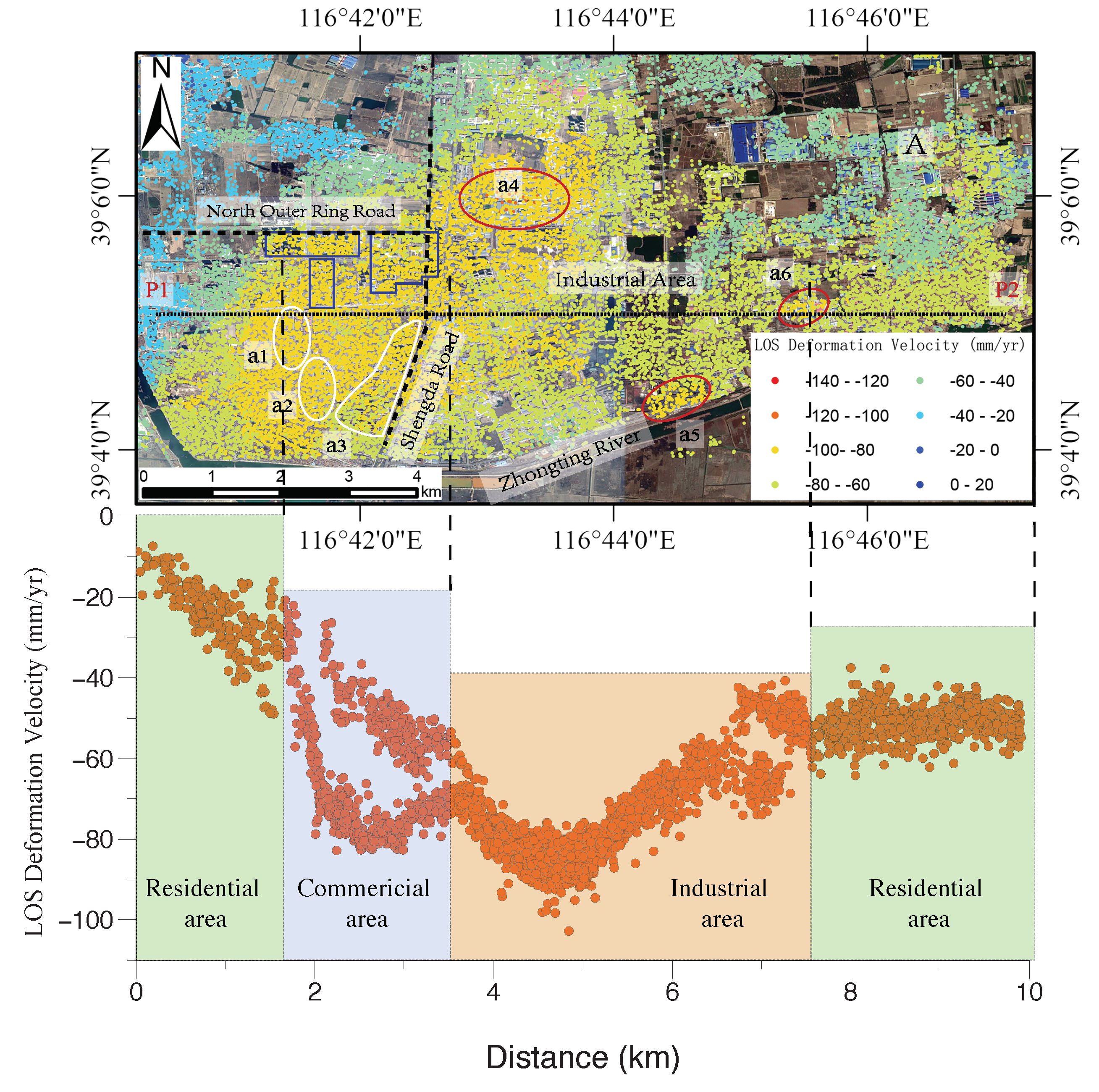
5.1. Subsidence Investigation and Their Causes

In order to better study the latest deformation velocities and trends of the serious subsidence funnels, and analyze its subsidence mechanism, the subsidence funnel of Part 1 in Figure 12 was enlarged as shown in Figure 13. It can be observed that most parts of the subsidence areas are located in and around Shengfang Town, Donggugang Town, and Wangqingtuo Town, and are distributed on both sides of the Rongcheng-Wuhai (i.e., Rongwu) highway and of the Tianjin-Baoding Intercity Railway. We can also see that the coverage area of Shengfang Town is not only the largest but also the one with the greatest area of subsidence. The most severe subsidence area was located in the western and north-eastern parts of Shengfang Town and in small portions of the eastern parts, showing an obvious regional subsidence pattern. The most serious subsidence area detected was located in Wangqingtuo Town, where the maximum subsidence velocity reached −136 mm/yr. The intercity railway from Tianjin to Baoding and the highway from Rongcheng to Wuhai are also affected by serious subsidence, and show obvious subsidence velocities in different sections. In order to figure out the subsidence mechanism, areas A, B, and C were enlarged, a well station has also been chosen to illustrate the variation of groundwater level, as shown in Figure 14, Figure 15 and Figure 16.

The subsidence in Tianjin might be caused by urban exploitation and geological influence. For Shengfang Town, urban development may play the most important role. The groundwater storage in Shengfang Town is abundant, but the shallow water is salt water, not suitable for irrigation. The deep groundwater has low mineralization and is widely exploited. There are 26 different types of industrial districts with more than 5200 industrial enterprises in this town. These are mainly furniture manufacturing and steel factories. As shown in Figure 14, the factories are mainly distributed in the north part of the North Outer Ring Road and east of Shengda Road. Most of these are furniture factories and there is a dense residential area located west of Shengda Road. A distinct subsidence funnel was detected in Zones a1 to a6 and in the Blue Line Zone. It can be seen that the subsidence rates in the a1, a2, and a3 commercial areas and near the new high-rise buildings in the south part of the North Outer Ring Road are much more serious than in the surrounding area (−110 mm/yr to −83 mm/yr). There has been little research on Shengfang Town, especially geological strata in this area. We have obtained a small amount of soil data from the Government development document. The document indicates that the soil in the north part of Zhongting River is lacustrine sediment, mainly fine silt and fine medium sand. Typically, in the centre of Shengfang Town, the soil is miscellaneous fill and the bearing capacity of such foundations is small, merely about 6 to 8 ton/m${}^2$. This weakness could easily lead to subsidence in major loading areas with intensive construction of buildings.

The north of the North Outer Ring Road is the old industrial district, most of the factories in this area are operating poorly, and some have already faced production suspension or closed down. However, the factories east of Shengda Road are operating well and most of these factories are new enterprises. Figure 14 illustrates that a high density of PS pixels were finally identified and less serious subsidence rates are detected in the new industrial district (−66 mm/yr to −10 mm/yr) than the old area (−110 mm/yr to −60 mm/yr). Furthermore, serious subsidence funnels were detected in Zones a4, a5, and a6. After investigating, we found that these factories are mainly for metal processing and glass manufacturing, so excessive groundwater exploitation may be the main cause of the differences in subsidence. In order to monitor the variation of groundwater level caused by the over exploitation of groundwater, a number of well stations have been built in different areas. A well station has been chosen to illustrate the variation of groundwater level, as shown in Figure 15.

Figure 15 shows that, apart from the visually prominent seasonal oscillations, a long-term linear trend was also detected in the time series. It indicates that the groundwater level has decreased year by year, mostly caused by the consumption of groundwater. This is even though the well station is located in Xiqing District, about 45 kilometers away from Shengfang Town. However, both of these areas are industrial cities, and Figure 12 shows that the subsidence in Shengfang Town and Wangqingtuo Town are the most severe in the study area. Therefore, the groundwater level variation in Xiqing District could also represent the groundwater level variation trend in Shengfang Town and Wangqingtuo Town to some extent.

To better study the surface deformation for the whole town, a profile line from point P1 to point P2 along the direction of the town was selected. The mean LOS deformation velocity of the profile is shown in Figure 14. It indicates that ground subsidence rates change with the different types of land use, as indicated by good correlation. In residential areas mainly located east and west of Shengfang Town, the subsidence rates range from −10 mm/yr to −60 mm/yr. The subsidence rates in the commercial areas are more serious than in the residential areas, with subsidence rates ranging from −30 mm/yr to −90 mm/yr. The most serious subsidence area is the industrial area, where the maximum subsidence rate reached −110 mm/yr. In 2017, Guo et al. [48] used a total of 27 Sentinel-1A images over Tianjin acquired between 31 May 2015 and 13 May 2016 to derive the subsidence of Tianjin. They found that the maximum subsidence rates have reached about −80mm/yr. The subsidence rate is further accelerating during 2016 to 2017. This result shows that the ground subsidence there is mainly caused by surface loads and groundwater extraction. In Shengfang Town, due to the large number of factories, the subsidence caused by over exploitation of groundwater is more serious.

5.2. Influence of Geological Factors on Subsidence

Region B and C have also been enlarged in Figure 16. We can see different subsidence rates on both sides of Line L1 and Line L2.

In Donggugang Town, some research has indicated that a rock layer was found when drilling at a depth of 100 m. Thus, different geological conditions may cause the differential subsidence rates on two sides of Line L1 [62]. Although much research has been carried out on subsidence in Wangqingtuo Town, little attention has focused on these differences. Here, hydrological and geological factors were analysed to discover the reason for the differences. The geological and hydrological map of Wangqingtuo Town is shown in Figure 17.

Figure 17 shows that the aquifer can be divided into four layers [62], with the first to fourth layers under Wangqingtuo Town at depths of 30 to 70 m, 180 to 220 m, 280 to 320 m and 370 to 430 m, respectively. A single well has also been used to assess the water abundance, and the experimental evidence suggests that the water yield property of the first layer is less than 100 m${}^3$/d and that the other three layers are in a relatively strong class (1000 to 3000 m${}^3$/d). This means that more space is needed between wells when drilling for equal amounts of groundwater from the different aquifers. This may lead to more serious subsidence while extracting shallow groundwater from the first aquifer than while extracting the deep phreatic water in Wangqingtuo Town. The areas in Wangqingtuo Town have the same geological conditions, so the differences of subsidence rates between the residential area and the industrial area may be due to the depth of the wells. For factories which require a large amount of water, it may be that only the deep, plentiful phreatic water can meet its production needs. In contrast, the shallow groundwater could meet the demand for water consumption in residential areas. This could be a good explanation for the differences in subsidence. Of course, with further improvement of the water supply system, it is also possible that the industrial water is derived from wells located in the main urban area. These are also likely to lead to the present subsidence differences. In order to get better and rational interpretations, more field trips need to be conducted and more relevant data need to be obtained.

Excessive extraction of groundwater is the main contributor to the subsidence in Tianjin. However, different geological conditions can also contribute to different degrees of subsidence. As Figure 16 illustrates, there are distinct differences in the subsidence rates within Donggugang Town and Wangqingtuo Town. Subsidence is more serious in Wangqingtuo Town than in Donggugang Town, and the maximum difference could reach 46 mm/yr. Generally, sediments underground to depths of about 20 to 30 m (e.g., Holocene) have great influence on the degree of subsidence, especially where shallow groundwater is withdrawn. The surface sediment of Wangqingtuo Town is alluvial–diluvial, which is composed of fine sand and silty sand with high porosity. The surrounding areas are formed by alluvium and lacustrine deposits, which are mainly composed of clay with low porosity. Therefore, subsidence is more likely to happen in Wangqingtuo Town when the same amount of groundwater is withdrawn in the two areas [62].

Additionally, since 2006, the groundwater exploitation in Wangqingtuo Town has extended from the third aquifer to the first aquifer and the amount of groundwater mining has also been increasing. Particularly in 2008, the amount of groundwater mining of the second aquifer was increased by about 26% relative to 2007, while use of the shallow aquifer was increased to 900,000, accounting for 36% of the total volume. Therefore, it is suggested that the continuing and increasing consumption of the shallow groundwater could accelerate the subsidence rates in Wangqingtuo Town, and that different geological conditions also have an important effect on surface subsidence.

6. Conclusions

In this study, we first applied StaMPS MT-InSAR methodology to Sentinel-1A TOPS SAR scenes collected from 9 January 2016 to 8 June 2017, to detect spatial and temporal ground deformation across the city of Tianjin. The evaluation of the results of the deformation in the Tianjin area suggests that the accuracy is very high in most of the area. The root mean square (RMS) reached 5.015 mm/yr and the standard deviation reached 5 mm/yr for 60.720 % of the PS points, except for the edge region where three-dimensional phase unwrapping cannot be well constrained. Furthermore, the InSAR-derived deformation time series show good agreement with the GPS time series, especially for the long-term trends, and present good consistency with each other.

This study shows that significant deformation has occurred in different parts of the Tianjin area, gradually increasing from the central part of the metropolitan areas toward the suburbs. The deformation rate of the main urban area is well-balanced and it is also relatively stable, with deformation rates ranging from 0 to 20 mm/yr in the LOS direction. This indicates that the Tianjin ground subsidence has been well controlled due to groundwater recharge by the government and factory migration in recent years. Remarkable subsidence funnels have also been detected in the eastern part of Tianjin, especially in Shengfang Town, Donggugang Town, and Wangqingtuo Town, with maximum subsidence rates reaching −120 mm/yr. Subsidence funnels in Wangqingtuo Town are mainly caused by intensive construction of buildings with heavy surface loading as well as industrial production with over exploitation of groundwater.

From the difference of subsidence rates in both Donggugang Town and Wangqingtuo Town, we draw the conclusion that different geological conditions also contribute to different degrees of subsidence, and that the maximum difference could reach 46 mm/yr. Shallow deposits formed by alluvial–diluvial sediment are more likely to exhibit subsidence than that by alluvium and lacustrine deposits in the case where the same amount of groundwater is withdrawn. Furthermore, obvious subsidence differences between the residential area and industrial area may demonstrate that differences in the depth of the wells used could also cause different subsidence rates, even in the same geological region.

References

1. Yin, Y.; Zuochen, Z.; Kaijun, Z. Land subsidence and countermeasures for its prevention in China. Chin. J. Geol. Hazard Control 2005, 16, 1–8. [Google Scholar]
2. Xue, Y.Q.; Zhang, Y.; Ye, S.J.; Wu, J.C.; Li, Q.F. Land subsidence in China. Environ. Geol. 2005, 48, 713–720. [Google Scholar] [CrossRef]
3. Dong, S.; Samsonov, S.; Yin, H.; Ye, S.; Cao, Y. Time-series analysis of subsidence associated with rapid urbanization in Shanghai, China measured with SBAS InSAR method. Environ. Earth Sci. 2013, 72, 677–691. [Google Scholar] [CrossRef]
4. Bai, L.; Jiang, L.; Wang, H.; Sun, Q. Spatiotemporal Characterization of Land Subsidence and Uplift (2009–2010) over Wuhan in Central China Revealed by TerraSAR-X InSAR Analysis. Remote Sens. 2016, 8, 350. [Google Scholar] [CrossRef]
5. Herrera, G.; Tomás, R.; Monells, D.; Centolanza, G.; Mallorquí, J.J.; Vicente, F.; Navarro, V.D.; Lopez-Sanchez, J.M.; Sanabria, M.; Cano, M. Analysis of subsidence using TerraSAR-X data: Murcia case study. Eng. Geol. 2010, 116, 284–295. [Google Scholar] [CrossRef]
6. Luo, S.M.; Shan, X.J.; Zhu, W.W.; Kai-Fu, D.U.; Wan, W.N.; Liang, H.B.; Liu, Z.G. Monitoring vertical ground deformation in the North China Plain using the multitrack PSInSAR technique. Chin. J. Geophys. 2014, 57, 3129–3139. [Google Scholar]
7. Wei, J.S.; Jia, X.U.; Yang, L.U.; Chang-Rong, Y.I. Analysis on Land Subsidence Funnel in Wangqingtuo Area of Tianjin. Ground Water 2012, 34, 49–51. [Google Scholar]
8. Gabriel, A.K.; Goldstein, R.M.; Zebker, H.A. Mapping small elevation changes over large areas: Differential radar interferometry. J. Geophys. Res. Solid Earth 1989, 94, 9183–9191. [Google Scholar] [CrossRef]
9. Ferretti, A.; Prati, C.; Rocca, F. Permanent scatterers in SAR interferometry. IEEE Trans. Geosci. Remote Sens. 2001, 39, 8–20. [Google Scholar] [CrossRef] [Green Version]
10. Sneed, M.; Stork, S.V.; Ikehara, M.E.; Galloway, D.L.; Amelung, F. Detection and measurement of land subsidence using Global Positioning System and interferometric synthetic aperture radar, Coachella Valley, California, 1996–98. Water-Resour. Investig. Rep. 2002, 8. [Google Scholar] [CrossRef]
11. Samsonov, S.; Marco, V.D.K.; Tiampo, K. A simultaneous inversion for deformation rates and topographic errors of DInSAR data utilizing linear least square inversion technique. Comput. Geosci. 2011, 37, 1083–1091. [Google Scholar] [CrossRef]
12. Crosetto, M.; Castillo, M.; Arbiol, R. Urban Subsidence Monitoring Using Radar Interferometry. Photogramm. Eng. Remote Sens. 2003, 69, 775–783. [Google Scholar] [CrossRef]
13. Metternicht, G.; Hurni, L.; Gogu, R. Remote sensing of landslides: An analysis of the potential contribution to geo-spatial systems for hazard assessment in mountainous environments. Remote Sens. Environ. 2005, 98, 284–303. [Google Scholar] [CrossRef]
14. Stramondo, S.; Cinti, F.R.; Dragoni, M.; Salvi, S. The August 17, 1999 Izmit, Turkey, earthquake: Slip distribution from dislocation modeling of DInSAR and surface offset. Ann. Geophys. 2002, 45, 527–536. [Google Scholar]
15. Guneriussen, T.; Hogda, K.A.; Johnsen, H.; Lauknes, I. InSAR for estimation of changes in snow water equivalent of dry snow. IEEE Trans. Geosci. Remote Sens. 2001, 39, 2101–2108. [Google Scholar] [CrossRef]
16. Zhou, L.; Guo, J.; Hu, J.; Li, J.; Xu, Y.; Pan, Y.; Shi, M. Wuhan Surface Subsidence Analysis in 2015–2016 Based on Sentinel-1A Data by SBAS-InSAR. Remote Sens. 2017, 9, 982. [Google Scholar] [CrossRef]
17. Zebker, H.A.; Rosen, P.A.; Hensley, S. Atmospheric Artifacts in Interferometric SAR Surface Deformation and Topographic Maps. J. Geophys. Res. Solid Earth 1997, 102, 7547–7563. [Google Scholar] [CrossRef]
18. Zebker, H.A.; Villasenor, J. Decorrelation in Interferometric Radar Echoes. IEEE Trans. Geosci. Remote Sens. 1992, 30, 950–959. [Google Scholar] [CrossRef]
19. Mora, O.; Mallorqui, J.J.; Broquetas, A. Linear and nonlinear terrain deformation maps from a reduced set of interferometric SAR images. IEEE Trans. Geosci. Remote Sens. 2003, 41, 2243–2253. [Google Scholar] [CrossRef]
20. Hooper, A.; Zebker, H.; Segall, P.; Kampes, B. A new method for measuring deformation on volcanoes and other natural terrains using InSAR persistent scatterers. Geophys. Res. Lett. 2004, 31, 1–5. [Google Scholar] [CrossRef]
21. Ferretti, A.; Savio, G.; Barzaghi, R.; Borghi, A.; Musazzi, S.; Novali, F.; Prati, C.; Rocca, F. Submillimeter Accuracy of InSAR Time Series: Experimental Validation. IEEE Trans. Geosci. Remote Sens. 2007, 45, 1142–1153. [Google Scholar] [CrossRef]
22. Berardino, P.; Fornaro, G.; Lanari, R.; Sansosti, E. A new algorithm for surface deformation monitoring based on small baseline differential SAR interferograms. IEEE Trans. Geosci. Remote Sens. 2002, 40, 2375–2383. [Google Scholar] [CrossRef]
23. Vilardo, G.; Ventura, G.; Terranova, C.; Matano, F.; Nardò, S. Ground deformation due to tectonic, hydrothermal, gravity, hydrogeological, and anthropic processes in the Campania Region (Southern Italy) from Permanent Scatterers Synthetic Aperture Radar Interferometry. Remote Sens. Environ. 2009, 113, 197–212. [Google Scholar] [CrossRef]
24. Vilardo, G.; Isaia, R.; Ventura, G.; Martino, P.D.; Terranova, C. InSAR Permanent Scatterer analysis reveals fault re-activation during inflation and deflation episodes at Campi Flegrei caldera. Remote Sens. Environ. 2010, 114, 2373–2383. [Google Scholar] [CrossRef]
25. Perissin, D.; Wang, T. Time-Series InSAR Applications Over Urban Areas in China. IEEE J. Sel. Top. Appl. Earth Observ. Remote Sens. 2011, 4, 92–100. [Google Scholar] [CrossRef]
26. Heleno, S.I.N.; Oliveira, L.G.S.; Henriques, M.J.; Falcão, A.P.; Lima, J.N.P.; Cooksley, G.; Ferretti, A.; Fonseca, A.M.; Lobo-Ferreira, J.P.; Fonseca, J.F.B.D. Persistent Scatterers Interferometry detects and measures ground subsidence in Lisbon. Remote Sens. Environ. 2011, 115, 2152–2167. [Google Scholar] [CrossRef]
27. Castellazzi, P.; Arroyo-Domínguez, N.; Martel, R.; Calderhead, A.I.; Normand, J.C.L.; Gárfias, J.; Rivera, A. Land subsidence in major cities of Central Mexico: Interpreting InSAR-derived land subsidence mapping with hydrogeological data. Int. J. Appl. Earth Observ. Geoinf. 2016, 47, 102–111. [Google Scholar] [CrossRef]
28. Hooper, A.; Segall, P.; Zebker, H. Persistent scatterer interferometric synthetic aperture radar for crustal deformation analysis, with application to Volcán Alcedo, Galápagos. J. Geophys. Res. Solid Earth 2007, 112. [Google Scholar] [CrossRef]
29. Massonnet, D.; Rossi, M.; Carmona, C.; Adragna, F.; Peltzer, G.; Feigl, K.; Rabaute, T. The displacement field of the Landers earthquake mapped by radar interferometry. Nature 1993, 364, 138–142. [Google Scholar] [CrossRef]
30. Li, Z.; Zhao, R.; Hu, J.; Wen, L.; Feng, G.; Zhang, Z.; Wang, Q. InSAR analysis of surface deformation over permafrost to estimate active layer thickness based on one-dimensional heat transfer model of soils. Sci. Rep. 2015, 5, 15542. [Google Scholar] [CrossRef] [PubMed] [Green Version]
31. Salvi, S.; Atzori, S.; Tolomei, C.; Allievi, J.; Ferretti, A.; Rocca, F.; Prati, C.; Stramondo, S.; Feuillet, N. Inflation rate of the Colli Albani volcanic complex retrieved by the permanent scatterers SAR interferometry technique. Geophys. Res. Lett. 2004, 31, 261–268. [Google Scholar] [CrossRef]
32. Motagh, M.; Shamshiri, R.; Haghighi, M.H.; Wetzel, H.U.; Akbari, B.; Nahavandchi, H.; Roessner, S.; Arabi, S. Quantifying groundwater exploitation induced subsidence in the Rafsanjan plain, southeastern Iran, using InSAR time-series and in situ measurements. Eng. Geol. 2017, 218, 134–151. [Google Scholar] [CrossRef]
33. Béjar-Pizarro, M.; Ezquerro, P.; Herrera, G.; Tomás, R.; Guardiola-Albert, C.; Hernández, J.M.R.; Merodo, J.A.F.; Marchamalo, M.; Martínez, R. Mapping groundwater level and aquifer storage variations from InSAR measurements in the Madrid aquifer, Central Spain. J. Hydrol. 2017, 547, 678–689. [Google Scholar] [CrossRef]
34. Ma, T.; Du, Y.; Ma, R.; Xiao, C.; Liu, Y. Review: Water–rock interactions and related eco-environmental effects in typical land subsidence zones of China. Hydrogeol. J. 2018, 26, 1339–1349. [Google Scholar] [CrossRef]
35. Matano, F.; Sacchi, M.; Vigliotti, M.; Ruberti, D. Subsidence Trends of Volturno River Coastal Plain (Northern Campania, Southern Italy) Inferred by SAR Interferometry Data. Geosciences 2018, 8, 8. [Google Scholar] [CrossRef]
36. Yang, Q.; Ke, Y.; Zhang, D.; Chen, B.; Gong, H.; Lv, M.; Zhu, L.; Li, X. Land Subsidence and Buildings: A Case Study in an Eastern Beijing Urban Area Using the PS-InSAR Technique. Remote Sens. 2018, 10, 1006. [Google Scholar] [CrossRef]
37. Bianchini, S.; Tapete, D.; Ciampalini, A.; Traglia, F.D.; Ventisette, C.D.; Moretti, S.; Casagli, N. Multi-Temporal Evaluation of Landslide-Induced Movements and Damage Assessment in San Fratello (Italy) by Means of C- and X-Band PSI Data. In Mathematics of Planet Earth; Springer: Berlin/Heidelberg, Germany, 2014; pp. 257–261. [Google Scholar]
38. Bianchini, S.; Raspini, F.; Solari, L.; Del Soldato, M.; Ciampalini, A.; Rosi, A.; Casagli, N. From Picture to Movie: Twenty Years of Ground Deformation Recording Over Tuscany Region (Italy) With Satellite InSAR. Front. Earth Sci. 2018, 6, 177. [Google Scholar] [CrossRef]
39. Raspini, F.; Bianchini, S.; Ciampalini, A.; Soldato, M.; Solari, L.; Novali, F.; Conte, S.; Rucci, A.; Ferretti, A.; Casagli, N. Continuous, semi-automatic monitoring of ground deformation using Sentinel-1 satellites. Sci. Rep. 2018, 8. [Google Scholar] [CrossRef]
40. Del Soldato, M.; Farolfi, G.; Rosi, A.; Raspini, F.; Casagli, N. Subsidence Evolution of the Firenze–Prato–Pistoia Plain (Central Italy) Combining PSI and GNSS Data. Remote Sens. 2018, 10, 1146. [Google Scholar] [CrossRef]
41. Zhou, C.; Gong, H.; Zhang, Y.; Warner, T.; Wang, C. Spatiotemporal Evolution of Land Subsidence in the Beijing Plain 2003–2015 Using Persistent Scatterer Interferometry (PSI) with Multi-Source SAR Data. Remote Sens. 2018, 10, 552. [Google Scholar] [CrossRef]
42. Xu, B.; Feng, G.; Li, Z.; Wang, Q.; Wang, C.; Xie, R. Coastal Subsidence Monitoring Associated with Land Reclamation Using the Point Target Based SBAS-InSAR Method: A Case Study of Shenzhen, China. Remote Sens. 2016, 8, 652. [Google Scholar] [CrossRef]
43. Solari, L.; Del Soldato, M.; Bianchini, S.; Ciampalini, A.; Ezquerro, P.; Montalti, R.; Raspini, F.; Moretti, S. From ERS 1/2 to Sentinel-1: Subsidence Monitoring in Italy in the Last Two Decades. Front. Earth Sci. 2018, 6, 149. [Google Scholar] [CrossRef]
44. Tomás, R.; Romero, R.; Mulas, J.; Marturià, J.; Mallorquí, J.; López-Sánchez, J.; Herrera, G.; Gutiérrez, F.; González, P.; Fernández, J. Radar interferometry techniques for the study of ground subsidence phenomena: A review of practical issues through cases in Spain. Environ. Earth Sci. 2014, 71, 163–181. [Google Scholar] [CrossRef]
45. Jia, S.X.; Zhang, C.K.; Zhao, J.R.; Fang, S.M.; Liu, Z.; Zhao, J.M. Crustal structure of the rift-depression basin and Yanshan uplift in the northeast part of North China. Chin. J. Geophys. 2009, 52, 99–110. [Google Scholar] [CrossRef]
46. Liu, P.; Li, Q.; Li, Z.; Hoey, T.; Liu, G.; Wang, C.; Hu, Z.; Zhou, Z.; Singleton, A. Anatomy of Subsidence in Tianjin from Time Series InSAR. Remote Sens. 2016, 8, 266. [Google Scholar] [CrossRef]
47. Lixin, Y.; Fang, Z.; He, X.; Shijie, C.; Wei, W.; Qiang, Y. Land subsidence in Tianjin, China. Environ. Earth Sci. 2011, 62, 1151–1161. [Google Scholar] [CrossRef]
48. Guo, J.; Hu, J.; Li, B.; Zhou, L.; Wang, W. Land subsidence in Tianjin for 2015 to 2016 revealed by the analysis of Sentinel-1A with SBAS-InSAR. J. Appl. Remote Sens. 2017, 11, 026024. [Google Scholar] [CrossRef]
49. Czikhardt, R.; Papco, J.; Bakon, M.; Liscak, P.; Ondrejka, P.; Zlocha, M. Ground Stability Monitoring of Undermined and Landslide Prone Areas by Means of Sentinel-1 Multi-Temporal InSAR, Case Study from Slovakia. Geosciences 2017, 7, 87. [Google Scholar] [CrossRef]
50. Lyons, S.; Sandwell, D. Fault creep along the southern San Andreas from interferometric synthetic aperture radar, permanent scatterers, and stacking. J. Geophys. Res. Solid Earth 2003, 108. [Google Scholar] [CrossRef] [Green Version]
51. Kampes, B. Displacement Parameter Estimation Using Permanent Scatterer Interferometry. Ph.D. Thesis, Delft Univ. of Technol., Delft, The Netherlands, 2005. [Google Scholar]
52. Hooper, A. A multi-temporal InSAR method incorporating both persistent scatterer and small baseline approaches. Geophys. Res. Lett. 2008, 35, 96–106. [Google Scholar] [CrossRef]
53. Kampes, B.M. Radar Interferometry: Persistent Scatterer Technique; Springer Publishing Company, Incorporated: New York, NY, USA, 2014. [Google Scholar]
54. Yang, C.; Zhang, Q.; Lu, Z.; Zhao, C.; Peng, J.; Ji, L. Deformation at Longyao Ground Fissure and its Surroundings Revealed by ALOS PALSAR PS-InSAR, North China Plain. In Proceedings of the AGU Fall Meeting, New Orleans, LA, USA, 11–15 December 2017. [Google Scholar]
55. Sousa, J.J.; Ruiz, A.M.; Hanssen, R.F.; Bastos, L.; Gil, A.J.; Galindo-Zaldívar, J.; Galdeano, C.S.D. PS-InSAR processing methodologies in the detection of field surface deformation—Study of the Granada basin (Central Betic Cordilleras, southern Spain). J. Geodyn. 2010, 49, 181–189. [Google Scholar] [CrossRef]
56. Hung, W.C.; Hwang, C.; Chen, Y.A.; Chang, C.P.; Yen, J.Y.; Hooper, A.; Yang, C.Y. Surface deformation from persistent scatterers SAR interferometry and fusion with leveling data: A case study over the Choushui River Alluvial Fan, Taiwan. Remote Sens. Environ. 2011, 115, 957–967. [Google Scholar] [CrossRef]
57. Hooper, A.J. Persistent Scatter Radar Interferometry for Crustal Deformation Studies and Modeling of Volcanic Deformation; Stanford University: Stanford, CA, USA, 2006. [Google Scholar]
58. Rocca, F. Modeling Interferogram Stacks. IEEE Trans. Geosci. Remote Sens. 2007, 45, 3289–3299. [Google Scholar] [CrossRef]
59. Colesanti, C.; Ferretti, A.; Novali, F.; Prati, C. SAR monitoring of progressive and seasonal ground deformation using the permanent scatterers technique. IEEE Trans. Geosci. Remote Sens. 2003, 41, 1685–1701. [Google Scholar] [CrossRef]
60. Zan, F.D.; Rocca, F. Coherent processing of long series of SAR images. In Proceedings of the 2005 IEEE International Geoscience and Remote Sensing Symposium, Seoul, Korea, 25–29 July 2005; pp. 1987–1990. [Google Scholar]
61. Hanssen, R.F. Radar Interferometry Data Interpretation and Error Analysis. J. Grad. School Chin. Acad. Sci. 2001, 2, V5-577–V5-580. [Google Scholar]
62. Luo, Q.; Perissin, D.; Zhang, Y.; Jia, Y. L- and X- band Multi-temporal InSAR Analysis of Tianjin. Remote Sens. 2014, 6, 7933–7951. [Google Scholar] [CrossRef]
63. Luo, Q.; Perissin, D.; Lin, H.; Zhang, Y.; Wang, W. Subsidence Monitoring of Tianjin Suburbs by TerraSAR-X Persistent Scatterers Interferometry. IEEE J. Sel. Top. Appl. Earth Obs. Remote Sens. 2014, 7, 1642–1650. [Google Scholar] [CrossRef]
Figure 1. This satellite image shows the location of the study area in our research and the red line is the provincial boundary. The pink rectangular frame denotes the coverage of the Sentinel-1A image and the red triangles represent the distribution of GPS stations.
Remotesensing 11 00130 g001
Figure 2. The tectonic framework of the study area. Piedmont plain, alluvial fan and flood plain, and coastal plain in North China Plain are bounded by thick red and blue lines. Major faults and subsidiary faults are shown in thick yellow and black solid lines, respectively. (Revised from [46])
Remotesensing 11 00130 g002
Figure 3. Temporospatial baseline distribution of ascending Sentinel-1A interferograms. The vertical axis shows the space perpendicular baseline in metres, the horizontal axis shows the image acquisition dates. All of the baselines represent interferometric pairs used for the time-series analysis. The green triangle represents the master image and the blue asterisks represent the slave images.
Remotesensing 11 00130 g003
Figure 4. Distribution of the calculated temporal coherence γ ^ for all of the PS pixels: The X-axis and Y-axis denote the coordinates of PS pixels in the direction of Azimuth and Range, respectively. The color scale shows the temporal correlation ranges from ‘0’ to ‘1’.
Remotesensing 11 00130 g004
Figure 5. The blue line shows the relationship between the temporal coherence γ ^ and the theoretical value of the velocity accuracy σ v for PS points (i.e., left-hand vertical axis). The histogram represents the statistic for the calculated coherence of PS points (i.e., right-hand vertical axis).
Remotesensing 11 00130 g005
Figure 6. Distribution of the standard deviation of the velocity for PS points in the direction of LOS.
Remotesensing 11 00130 g006
Figure 7. Theoretical and calculated statistics of the standard deviation of the mean velocity for PS points in the direction of LOS. Blue histogram denotes the theoretical statistics (left axis) and the red histogram denotes the calculated statistics (right axis).
Remotesensing 11 00130 g007
Figure 8. Comparison of the original and filtered GPS vertical deformation time series. The grey line denotes the original GPS time series and the red line denotes the time series filtered with a Db3 wavelet.
Remotesensing 11 00130 g008
Figure 9. Signal-to-noise ratio of the original and filtered GPS time series. The blue line denotes the SNR of the original GPS time series and the red line denotes the SNR of the time series filtered with a Db3 wavelet.
Remotesensing 11 00130 g009
Figure 10. Comparison between GPS time series and Sentinel-1A derived LOS deformation time series. The velocities of the GPS sites were projected in the LOS direction. The red line represents the filtered time series of GPS stations, black dotted line represent the 95% confidence interval, and the asterisk represents the InSAR-derived time series for the corresponding PS points.
Remotesensing 11 00130 g010
Figure 11. Time series of the vertical deformation for Tianjin from 26 February 2016 to 8 June 2017 referenced temporally to the earliest image (9 January 2016) and referenced spatially to a stable CORS station (JIXN) located in the north-east corner of Tianjin.
Remotesensing 11 00130 g011
Figure 12. Linear deformation trend derived by PS technique along the LOS direction of ascending pairs, blue triangle denotes the reference point, red triangles denote the GPS stations and the double circles denote the well station ZDK. Each administrative region and severely deformation areas are marked in black font. 1–5 represent five major subsidence areas which enclosed by red lines. Two surface uplifting areas are also represent by blue ovals.
Remotesensing 11 00130 g012
Figure 13. The mean LOS deformation velocity of the subsidence funnel over Part 1 as shown in Figure 12: The white boxes A, B, and C represent Shengfang, Donggugang and Wangqingtuo Town, respectively. The red lines L1 and L2 represent the borders of different subsidence velocities.
Remotesensing 11 00130 g013
Figure 14. The mean LOS deformation velocity map over Shengfang Town, Part A, as shown in Figure 13. Zones a1, a2, and a3 represent commercial zones in Shengfang. The red ellipses indicate Zones a4, a5, and a6 where subsidence velocities are different from those in the surrounding areas and where there are many steel factories. The blue line represents the new residential district. The black dotted line from point P1 to P2 is the profile of Shengfang Town.
Remotesensing 11 00130 g014
Figure 15. Groundwater level variation of the well station ZDK. The location of this station has been given in Figure 12. Red dotted line denotes the time span for the Sentinel data acquisition. Vertical axis denotes the measured values, which is contrary to the actual groundwater level.
Remotesensing 11 00130 g015
Figure 16. The mean LOS deformation velocity map of Shengfang Town and Wangqingtuo Town: The black dotted line from point P3 to P4 represent the profile of the Jintong Road.
Remotesensing 11 00130 g016
Figure 17. (a) Geological map of Wangqingtuo Town, (b) Geological profile map (above) and Hydrological profile map (below). The black box in panel b denotes the span in the direction from north-west to south-east, W1 denotes Wangqingtu Town, W2 and W3 denote Xiqing District, the red dotted line L3 in the panel a denotes the profile from W1 to W3. This figure is revised from [62,63].
Remotesensing 11 00130 g017