A Unified Model for Multi-Frequency PPP Ambiguity Resolution and Test Results with Galileo and BeiDou Triple-Frequency Observations

Abstract

With the modernization of Global Navigation Satellite System (GNSS), triple- or multi-frequency signals have become available from more and more GNSS satellites. The additional signals are expected to enhance the performance of precise point positioning (PPP) with ambiguity resolution (AR). To deal with the additional signals, we propose a unified modeling strategy for multi-frequency PPP AR based on raw uncombined observations. Based on the unified model, the fractional cycle biases (FCBs) generated from multi-frequency observations can be flexibly used, such as for dual- or triple- frequency PPP AR. Its efficiency is verified with Galileo and BeiDou triple-frequency observations collected from globally distributed MGEX stations. The estimated FCB are assessed with respect to residual distributions and standard deviations. The obtained results indicate good consistency between the input float ambiguities and the generated FCBs. To assess the performance of the triple-frequency PPP AR, 11 days of MGEX data are processed in three-hour sessions. The positional biases in the ambiguity-fixed solutions are significantly reduced compared with the float solutions. The improvements are 49.2%, 38.3%, and 29.6%, respectively, in east/north/up components for positioning with BDS, while the corresponding improvements are 60.0%, 29.0%, and 21.1% for positioning with Galileo. These results confirm the efficiency of the proposed approach, and that the triple-frequency PPP AR can bring an obvious benefit to the ambiguity-float PPP solution.

1. Introduction

Precise point positioning (PPP) has found increased applications due to its cost-effectiveness, global coverage, and high accuracy [1,2]. Usually PPP is able to achieve a positional accuracy of 10 cm after a convergence time of 30 min [3]. The integer ambiguity resolution (AR) technique is expected to further enhance the accuracy and shorten the convergence time [4,5]. In addition, [6] shows that the Galileo orbit determination could be improved when employing AR in multiple Global Navigation Satellite System (GNSS) data processing. However, the uncalibrated phase delays (UPDs) originating from satellites and receivers destroy the integer nature of PPP ambiguities. By determining the UPDs, to be estimated as fractional cycle biases (FCBs) at the server end and applying them at the user end, the PPP integer ambiguity resolution could become feasible [7,8,9]. Similarly, the decoupled clock model [10] and the integer phase clock model [11] were developed. These PPP AR techniques have been proven equivalent in theory [12,13], and the positional biases have been demonstrated to be minimal [14]. Beside GPS, PPP AR has been extended to GLONASS [15,16,17], BeiDou Navigation Satellite System (BDS) [18,19], Galileo [20,21], and multi-GNSS [22].

As to the functional models used for PPP, the dual-frequency ionospheric-free (IF) combination is routinely employed (e.g., in the above-mentioned research). However, with emerging BDS and Galileo, as well as the modernization of GPS and GLONASS, various types of multi-frequency observables become available [23]. The choice of optimum combinations then becomes practically difficult given the diversity of equipment [24]. In addition, the IF combination will amplify the measurement noise level by a factor of about 3, which will degrade the performance of the position solution. As a result, the PPP model based on uncombined measurements, in which the individual signal of each frequency is treated as an independent observable, has drawn increasing interest in the GNSS community [25]. Its efficiency has already been confirmed in terms of convergence time and precision for single-frequency PPP [26], multi-GNSS PPP [27], as well as PPP-RTK [28,29]. Moreover, this approach has been tested effectively for ionospheric modelling [30,31], differential code bias (DCB) estimation [32,33], and low earth satellite orbit determination [34].

Compared to the well-developed IF PPP model, the uncombined PPP model, called uncombined PPP in the sequel, requires more investigation, especially in the case of multi-frequency processing and ambiguity resolution. First, how to model and constrain the ionospheric delay has a crucial impact on performance using the uncombined PPP. For example, it has been demonstrated that a white noise model is not adequate to capture the characteristics of the ionospheric delay. The external constraints developed from the ionospheric products, such as the IGS global ionosphere maps, are also not accurate enough to completely separate the ionospheric effects from the ambiguity parameters [25]. The influence of the ionospheric effects on the ambiguity fixing therefore must be reduced. Second, the method to deal with the DCB errors is more problematic with the uncombined PPP [35] than the dual-frequency IF PPP, since the latter can cancel out the DCB biases. The problem of partial assimilation of the code bias (DCB) into phase bias (FCB) should also be carefully considered. Third, the uncombined PPP approach was proposed to deal with multi-GNSS and multi-frequency signals, so a generalized FCB estimation and AR method [36], which is extendable to dual-, triple-, and multi- frequency, should be proposed.

Li et al. [37] verified the feasibility of the uncombined PPP AR with refined ionospheric models. The ionospheric delay was constrained from a priori spatial-temporal information and ionospheric products. The GPS dual-frequency ambiguities were fixed sequentially in the forms of wide-lane (WL)/narrow-lane (NL), which followed the convention of IF PPP AR. Gu et al. [38] further testified the uncombined PPP AR with BDS triple-frequency observations. The extra-wide-lane (EWL) and WL ambiguities were successfully fixed, whereas the B1 ambiguities were kept as float values. In addition, the performance was further limited by the satellite-induced multipath effects [39]. Li, Zhang, Ge, and Schuh [36] proposed a unified FCB estimation and PPP AR method, which is extendable to multi-frequency uncombined PPP. The FCBs on each frequency were directly estimated from the raw float ambiguities derived from triple frequency observables. The model showed a great potential for multi-frequency uncombined PPP AR, although its DCB strategy may not be optimal. The satellite DCBs, together with the receiver DCB, were estimated as unknowns, and as a result the number of unknown parameters was increased. Given that the satellite GNSS DCB product is currently available on a routine basis [40], it would be beneficial to make use of these products. In addition, validating the method with Galileo observations is of interest considering the recent and rapid development of Galileo.

The aim of this study is to develop a unified modeling strategy for multi-frequency and multi-GNSS uncombined PPP AR. The unified model is able to generate consistent FCB products and perform PPP AR for multi-frequency PPP. The proposed approach will be first described, and its effectiveness will be verified with Galileo and BDS triple-frequency observations collected from the globally distributed Multi-GNSS EXperiment (MGEX) stations. The estimated FCB are assessed with respect to residual distributions and standard deviations, followed by an evaluation of the performance improvements in Galileo and BDS triple-frequency PPP AR. Finally, the results are summarized, and an outlook for future research is presented.

2. Methodology

The proposed uncombined PPP mode will be first described in this section, followed by a description of our FCB estimation strategy. With the obtained FCB products, the uncombined PPP AR algorithm at the user end is then elaborated.

2.1. Uncombined PPP Float Ambiguity Model

In the classic GNSS dual-frequency PPP, the first-order ionospheric delay is eliminated by the formation of the IF combination [2]. In the uncombined PPP model, the ionospheric delay is directly estimated. For a satellite s observed by receiver r, the corresponding raw pseudo-range and carrier phase observation equations can be expressed as [41]

$$\{\begin{array}{l}{P}_{r,f}^s={\rho }_r^s+d{t}_r-d{t}^s+dT+a_f·d{I}_{r,1}^s+D_{r,f}-D_f^s+{\epsilon }_{P_f} \\ {\Phi }_{r,f}^s={\rho }_r^s+d{t}_r-d{t}^s+dT-a_f·d{I}_{r,1}^s+{\lambda }_f\left(N_{r,f}^s+B_{r,f}-B_f^s\right)+{\epsilon }_{{\Phi }_f}\end{array}$$

(1)

where the subscript $f=\left(1,2,3,\cdots \right)$ refers to a specific carrier frequency, superscript $s$ refers to a specific satellite; ${\rho }_r^s$ indicates the geometric distance between the satellite and receiver; $d{t}_r$ and $d{t}^s$ are the clock errors of receiver and satellite; $dT$ is the slant tropospheric delay; $d{I}_{r,1}^s$ is the slant ionospheric delay on the first carrier frequency and $a_f={\lambda }_f^2/{\lambda }_1^2$ is the carrier frequency-dependent factor; $D_{r,f}$ and $D_f^s$ are the receiver and satellite specific code hardware delays; ${\lambda }_f$ and $N_{r,f}^s$ are the wavelength in meter and integer ambiguity in cycle; $B_{r,f}$ and $B_f^s$ are the receiver-dependent and satellite-dependent uncalibrated phase delays; ${\epsilon }_{P_f}$ and ${\epsilon }_{{\Phi }_f}$ are the pseudo-range and carrier phase measurement noise, respectively. Note that the higher-order ionospheric effects are neglected, as they have limited influence on the performance of ambiguity resolution [42].

Another important difference between the IF PPP and the uncombined PPP model is the strategy to deal with the DCB. The DCB is not of concern in IF PPP as the IF combination is also used for precise clock generation, which implies that the DCB could be fully absorbed by other parameters or simply cancelled out in the IF PPP [43]. But this is not the case in the uncombined PPP, especially with multi-frequency observations. Conventionally, precise orbit and clock products from the IGS analysis center are used to remove satellite orbit and clock errors. During the generation of precise clock products, the pseudo-range IF hardware delay bias $D_{IF}^s=\frac{a_2}{a_2-1}{D}_1^s-\frac{1}{a_2-1}{D}_2^s$ is assimilated into the clock offset $d{t}^s$ in accordance with the IGS analysis convention. After applying the GNSS precise satellite clock products, Equation (1) can be rewritten as

$$\{\begin{array}{l}{P}_{r,f}^s={\rho }_r^s+d{t}_r-d{t}_{pre}^s+dT+a_f·d{I}_{r,1}^s+D_{r,f}-D_f^s+D_{IF}^s+{\epsilon }_{P_f}\\ {\Phi }_{r,f}^s={\rho }_r^s+d{t}_r-d{t}_{pre}^s+dT-a_f·d{I}_{r,1}^s+{\lambda }_f\left(N_{r,f}^s+B_{r,f}-B_f^s\right)+D_{IF}^s+{\epsilon }_{{\Phi }_f}\end{array}$$

(2)

This linear system is rank-deficient due to the DCB parameters. For dual-frequency uncombined PPP processing, the singularities can be eliminated by a re-parameterization process. This is accomplished based on the fact that the DCB parameters can be separated into satellite-related, receiver-related, and frequency-related parts, and therefore can be fully absorbed, respectively, by satellite clock, receiver clock, and ionospheric parameters [31]. This method is efficient for dual-frequency processing but becomes complicated when facing multi-frequency observations. It is also possible to estimate these DCB parameters in advance. This is typically done by employing a network of receivers and imposing a zero-mean constraint. This option is complicated and not suitable for single receivers. In our study, we propose estimation of the receiver DCB and correction of the satellite DCB with existing multi-GNSS DCB products [40]. Taking triple-frequency observations as an example, the correction equation can be deduced as [35]

$$\{\begin{array}{l}{P}_{r,1}^s={\rho }_r^s+\overline{d}{t}_r-d{t}_{pre}^s+dT+a_1·d{I}_{r,1}^s-\frac{1}{a_2-1}DC{B}_{12}^s+{\epsilon }_{P_f}\\ P_{r,2}^s={\rho }_r^s+\overline{d}{t}_r-d{t}_{pre}^s+dT+a_2·d{I}_{r,1}^s-\frac{a_2}{a_2-1}DC{B}_{12}^s+DC{B}_{r,12}+{\epsilon }_{P_f}\\ P_{r,3}^s={\rho }_r^s+\overline{d}{t}_r-d{t}_{pre}^s+dT+a_3·d{I}_{r,1}^s-DC{B}_{13}^s-\frac{1}{a_2-1}DC{B}_{12}^s+DC{B}_{r,13}+{\epsilon }_{P_f}\end{array}$$

(3)

where $DC{B}_{12}^s=D_2^s-D_1^s$, $DC{B}_{r,12}=D_{r,2}-D_{r,1}$, and $\overline{d}{t}_r=d{t}_r+D_{r,1}$. The $DC{B}_{12}^s$ and $DC{B}_{13}^s$ can be obtained from multi-GNSS DCB products, while $DC{B}_{r,12}$ and $DC{B}_{r,13}$ are estimated as daily constant parameters. Similarly, the phase equations can be rewritten as

$${\Phi }_{r,f}^s={\rho }_r^s+\overline{d}{t}_r-d{t}_{pre}^s+dT-a_f·d{I}_{r,1}^s+{\lambda }_f{\overline{N}}_{r,f}^s+{\epsilon }_{{\Phi }_f}$$

(4)

where the ambiguity can be re-parameterized as

$$\{\begin{array}{l}{\overline{N}}_{r,f}^s=N_{r,f}^s+b_{r,f}-b_f^s \\ b_{r,f}=B_{r,f}-D_{r,1}/{\lambda }_f \\ b_f^s=B_f^s-D_{IF}^s/{\lambda }_f\end{array}$$

(5)

and the estimable parameters are

$$X=\left[\begin{array}{ccc}x& y& \begin{array}{ccc}z& \overline{d}{t}_r& \begin{array}{ccc}dT& I_{r,1}^s& \begin{array}{cc}{D}_{r,12}& \begin{array}{ccc}{D}_{r,13}& {\overline{N}}_{r,1}^s& \begin{array}{cc}{\overline{N}}_{r,2}^s& {\overline{N}}_{r,3}^s\end{array}\end{array}\end{array}\end{array}\end{array}\end{array}\right]$$

(6)

Compared with the model in Li, Zhang, Ge, and Schuh [36], the structure of the unknown parameters, except $\left(x,y,z\right)$, is different, due to the different strategies of DCB correction. In Li, Zhang, Ge, and Schuh [36], the dual-frequency DCBs are absorbed by other parameters, whereas the third frequency DCBs are estimated. In this study, the satellite DCBs for all the three frequencies are corrected with existing DCB products [40] and the receiver DCBs are estimated. Consequently, our ionospheric parameters will not be biased by DCBs, which is beneficial for ionospheric modelling. In addition, for single stations with n observable satellites, the number of DCB parameters to be estimated in their model is n, while it is 2 in our model. The degree of freedom of our model is larger, which could increase the redundancy and robustness of the positioning solutions. The estimated ambiguity parameter is a combination of the integer ambiguity, the corresponding code hardware delays, and the uncalibrated carrier phase delays at both receiver and satellite ends. In order to recover its integer property, these biases, i.e., satellite FCB $b_f^s$ and receiver FCB $b_{r,f}$, must be accounted for. Normally, the receiver FCB is not of concern as it can be eliminated when performing single differences of observations between satellites. The satellite FCB, however, must be estimated at the server end and broadcasted to the users.

2.2. FCB Estimation Strategy

In dual-frequency IF PPP, the float ambiguity is usually decomposed into WL/NL forms in order to recover the integer property [7]. This is partly because the IF combination of L1/L2 ambiguities is in essence not an integer. Another reason is that the WL ambiguities possess a relatively longer wavelength and are less correlated, therefore can be easily fixed. For uncombined PPP AR, it is also important to form combinations of raw ambiguities. On the one hand, the estimated raw float ambiguities are strongly correlated. On the other hand, the raw float ambiguities are quite sensitive to unmodeled ionospheric errors [25]. Therefore, the combinations with longer wavelength and lower ionospheric delay are preferred. The coefficients must be integers in order to preserve the integer nature of ambiguities. In addition, these combinations should be independent to avoid rank-deficiency. While the Least-squares AMBiguity Decorrelation Adjustment (LAMBDA) method can be used to automatically search for the optimal linear combinations of ambiguities [36,44], the classic extra-/wide-lane ambiguities (EWL/WL) were found to perform equally well and were used in our work to simplify the algorithm. For triple-frequency observations, it is easy to find two optimal combinations, e.g., one EWL and one WL combination or two WL combinations. The searching of the third combination, however, is much more difficult. From the systematic investigation of triple-frequency combinations, it is found that (4, −3, 0) is a good compromise between ionospheric reduction and noise amplification [36]. Concerning the properties of the above combinations shown in

Table 1. Properties of GPS, Galileo, and BDS triple-frequency linear combinations.

GNSS	Coefficients	Wavelength [meter]	Ionospheric Delay [cycle]	Noise [cycle]
GPS	(4, −3, 0)	0.114	0.150	5.0
	(1, −1, 0)	0.862	−0.283	1.414
	(1, 0, −1)	0.751	−0.339	1.414
Galileo	(4, −3, 0)	0.108	−0.017	5.0
	(1, −1, 0)	0.751	−0.339	1.414
	(1, 0, −1)	0.814	−0.305	1.414
BDS	(4, −3, 0)	0.114	0.120	5.0
	(1, −1, 0)	0.847	−0.293	1.414
	(1, 0, −1)	1.025	−0.231	1.414

, they are denoted as NL/WL/EWL without specific explanation herein. In addition, they are used for both BDS and Galileo triple-frequency observations for simplicity

$$\left[\begin{array}{c}{\overline{N}}_{r,LC1}^s\\ {\overline{N}}_{r,LC2}^s\\ {\overline{N}}_{r,LC3}^s\end{array}\right]=\left[\begin{array}{ccc}4& -3& 0\\ 1& -1& 0\\ 1& 0& -1\end{array}\right]\left[\begin{array}{c}{\overline{N}}_{r,1}^s\\ {\overline{N}}_{r,2}^s\\ {\overline{N}}_{r,3}^s\end{array}\right]$$

(7)

Substituting (5) into the above system produces the basic model for estimating FCBs. Since they have the same structure, a general expression can be formulated as

$$R_{r,LC}^s={\overline{N}}_{r,LC}^s-{\widehat{N}}_{r,LC}^s=d_{r,LC}-d_{LC}^s$$

(8)

for all linear combinations, ${\overline{N}}_{r,LC}^s$ denotes the float combined ambiguities; ${\widehat{N}}_r^s$ denotes the integer part of ${\overline{N}}_{r,LC}^s$; $d_{r,LC}$ and $d_{LC}^s$ denotes the receiver and satellite FCBs; $R_{r,LC}^s$ represents the FCB measurements. For each linear combination, a set of equations in the form of (8) can be generated, based on a network of reference stations. Suppose that there are n satellites tracked by m reference stations, the system of equations can be expressed as

$$\left[\begin{array}{c}{R}_{1,LC}^1\\ ⋮\\ R_{1,LC}^n\\ ⋮\\ R_{m,LC}^1\\ ⋮\\ R_{m,LC}^n\end{array}\right]=\left[\begin{array}{c}{\overline{N}}_{1,LC}^1-{\widehat{N}}_{1,LC}^1\\ ⋮\\ {\overline{N}}_{1,LC}^n-{\widehat{N}}_{1,LC}^n\\ ⋮\\ {\overline{N}}_{m,LC}^1-{\widehat{N}}_{m,LC}^1\\ ⋮\\ {\overline{N}}_{m,LC}^n-{\widehat{N}}_{m,LC}^n\end{array}\right]=\left[\begin{array}{cccccc}1& \cdots & 0& -1& \cdots & 0\\ ⋮& ⋮& ⋮& ⋮& \ddots & ⋮\\ 1& \cdots & 0& 0& \cdots & -1\\ ⋮& ⋮& ⋮& ⋮& ⋮& ⋮\\ 0& \cdots & 1& -1& \cdots & 0\\ ⋮& ⋮& ⋮& ⋮& \ddots & ⋮\\ 0& \cdots & 1& 0& \cdots & -1\end{array}\right]=\left[\begin{array}{c}{d}_{1,LC}\\ ⋮\\ d_{m,LC}\\ d_{LC}^1\\ ⋮\\ d_{LC}^n\end{array}\right]$$

(9)

where LC stand for the linear combinations $\left(LC1,LC2,LC3,\cdots \right)$. The obtained system is singular on both sides of the equations. For the left side, ${\widehat{N}}_{r,LC}^s$ can be determined by rounding ${\overline{N}}_{r,LC}^s$, assuming that the float ambiguities are precisely estimated. For the right side, one arbitrarily combined FCB should be set to zero. For all the linear combinations, we always set the combined FCB of the last satellite to zero, i.e., G32/E30/C14. Note that the FCB measurements $R_{r,LC}^s$ from different stations may differ with $\pm 1$ cycle. This is due to the rounding process and can be adjusted with the strategy described in Xiao, Sui, Heck, Zeng, and Tian [9]. In this way, the system of equations can be solved. With the obtained combined FCB, we are able to calculate the FCB of the raw L1/L2/L3 carrier frequency

$$\left[\begin{array}{c}{d}_1^s\\ d_2^s\\ d_3^s\end{array}\right]={\left[\begin{array}{ccc}4& -3& 0\\ 1& -1& 0\\ 1& 0& -1\end{array}\right]}^{-1}\left[\begin{array}{c}{d}_{LC1}^s\\ d_{LC2}^s\\ d_{LC3}^s\end{array}\right]$$

(10)

The transformation from combined FCBs to raw FCBs is important, as it provides more flexibility to the users. With the raw FCBs, users are able to choose their own linear combinations of observations, formulate the corresponding combined FCB, and conduct PPP AR. This representation allows interoperability if the server and user sides implement different AR methods. In addition, the raw FCB is suitable for the State Space Representation (SSR) of Radio Technical Commission for Maritime services (RTCM) [45], where one phase bias per phase observable is broadcasted instead of making specific combinations.

2.3. Uncombined PPP AR at the User End

Similar to dual-frequency IF PPP AR, single differencing across satellites must be firstly performed in order to remove receiver FCBs. Then the single-differenced ambiguities from different carrier frequencies are combined, as has been done during FCB estimation

$$\left[\begin{array}{c}{\overline{N}}_{r,ijk1}^{m,n}\\ {\overline{N}}_{r,ijk2}^{m,n}\\ {\overline{N}}_{r,ijk3}^{m,n}\end{array}\right]=\left[\begin{array}{ccc}{i}_1& j_1& k_1\\ i_2& j_2& k_2\\ i_3& j_3& k_3\end{array}\right]\left[\begin{array}{c}{\overline{N}}_{r,1}^{m,n}\\ {\overline{N}}_{r,2}^{m,n}\\ {\overline{N}}_{r,3}^{m,n}\end{array}\right]$$

(11)

where ${\overline{N}}_r^{m,n}={\overline{N}}_r^m-{\overline{N}}_r^n$ is the single-differenced ambiguity between satellites m and n. Based on the coefficients $\left(i,j,k\right)$, the FCB for the specific combined ambiguity can also be formed. Note that the linear combinations are not necessary to be the same as that in FCB estimation, although the three combinations mentioned above are strongly recommended. In our experiments, we have used the same combinations as in FCB generation for uncombined PPP AR.

Usually, the EWL/WL float ambiguities can be directly fixed by the rounding approach after the correction of FCB [7], and the NL float ambiguities are fed into the LAMBDA algorithm to search for correct integers [44]. However, in our study, the LAMBDA is used for each combination, regardless of its property, which simplifies the design of the algorithm. In addition, if not all the float ambiguities can be fixed by the LAMBDA method, partial ambiguity resolution can be employed [46,47]. It is found that the searching and fixing of ambiguities for the combination with longer wavelengths (e.g., EWL/WL) is quite fast. When the integer ambiguities for one combination are resolved and validated, a tight constraint can be reconstructed. The number of constraints accumulate as the process repeats for all linear combinations. Afterwards, the constraints are imposed on the raw ambiguities, and yields the AR solution. Note that the ambiguities in IF PPP AR must be sequentially fixed in the order of WL/NL. An IF ambiguity is constrained only when both its WL and NL ambiguities are fixed, while the linear combined ambiguities in our study can be fixed and constrained independently.

3. Results and Discussion

In this section, the data and processing strategy is described, followed by an analysis of the quality of triple-frequency FCB estimation. We further convert the combined FCB to raw FCB on each carrier frequency in order to characterize their properties. The generated FCBs are used to evaluate the performance of triple-frequency PPP AR solutions.

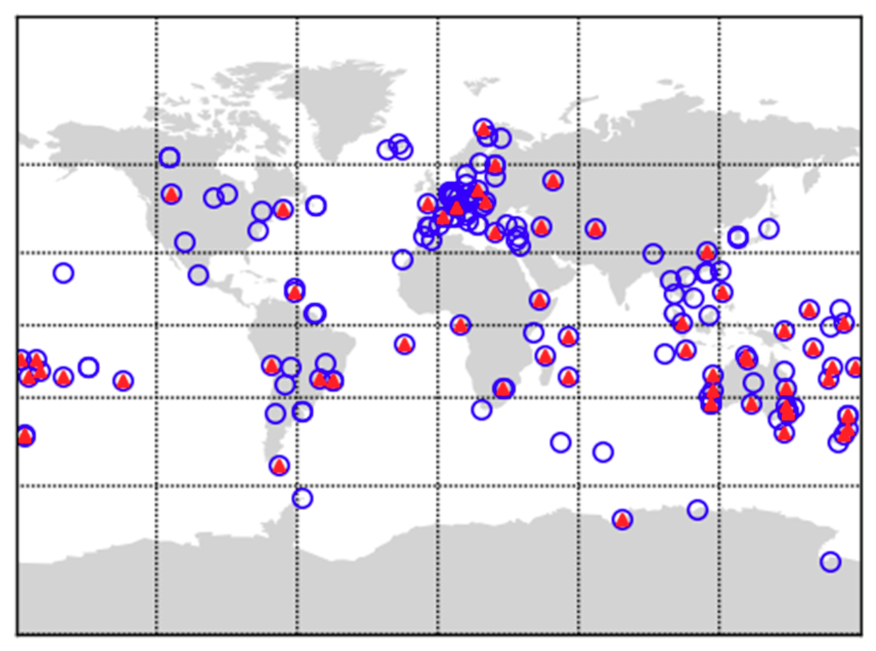
3.1. Data and Processing Strategy

The International GNSS Service (IGS) established the MGEX in order to prepare operational services for new and upcoming GNSS [23]. The MGEX network comprises over 220 MGEX stations, as of October 2017. The daily observations from 7 September–27 October 2017—in total 51 days—were collected. About 200 stations were used for Galileo FCB estimation, of which 160 stations provide E1/E5a/E5b triple-frequency observations. About 150 stations were used for BDS FCB estimation, of which 60 stations provide B1/B2/B3 triple-frequency observations. Figure 1 shows the geographic distribution of the MGEX stations with Galileo and BDS triple-frequency observations. These data provide almost full and continuous tracking of Galileo and BDS signals.

In the processing, the E1/E5a/E5b were used for Galileo, while B1/B2/B3 were used for BDS. Data from GPS L1/L2 was also used to test the efficiency of the proposed approach in the case of dual-frequency observations, while the L3 was excluded due to inter-frequency clock bias [48]. The cut-off elevation angle was set to 10°, while the float ambiguities with an elevation below 30° or with standard deviation (STD) larger than 0.1 m were removed for FCB estimation. It is noted that the BDS satellite-induced code multipath effects were corrected for inclined geosynchronous orbit (IGSO) and medium earth orbit (MEO) satellites, according to Wanninger and Beer [39], while geostationary orbit (GEO) satellites were excluded from the processing. The third-generation BDS satellites, which were no longer affected by such effects [49], were also excluded due to no public data. Throughout the processing, MGEX precise products provided by Deutsches GeoForschungsZentrum (GFZ) [50] were used. The satellite phase center offsets and variations were corrected according to the IGS antenna file. Since the antenna correction values for the third frequency, i.e., E5b and B3, were not available, we simply used that of the second frequency, i.e., E5a/B2. It is demonstrated that the satellite antenna characteristics of the third carrier frequency were quite similar to those of the second carrier frequency [24]. However, it is a compromised strategy considering the precision of phase measurements. We have downweighed the observations of the third frequency by a factor of 4, compared with that of the first and the second carrier frequency. As for the receiver antenna phase center offsets and variations, the correction values for GPS were employed for both Galileo and BDS, in accordance with the principle of orbit and clock generation [51]. For the combined GPS, Galileo, and BDS processing, the system related weighting ratio of GPS, Galileo, and BDS code observations was assumed to be 1:1:3, while the precision of the phase observations was assumed to be at the same level [52]. The detail of the used software and processing standards can be found in [9,21].

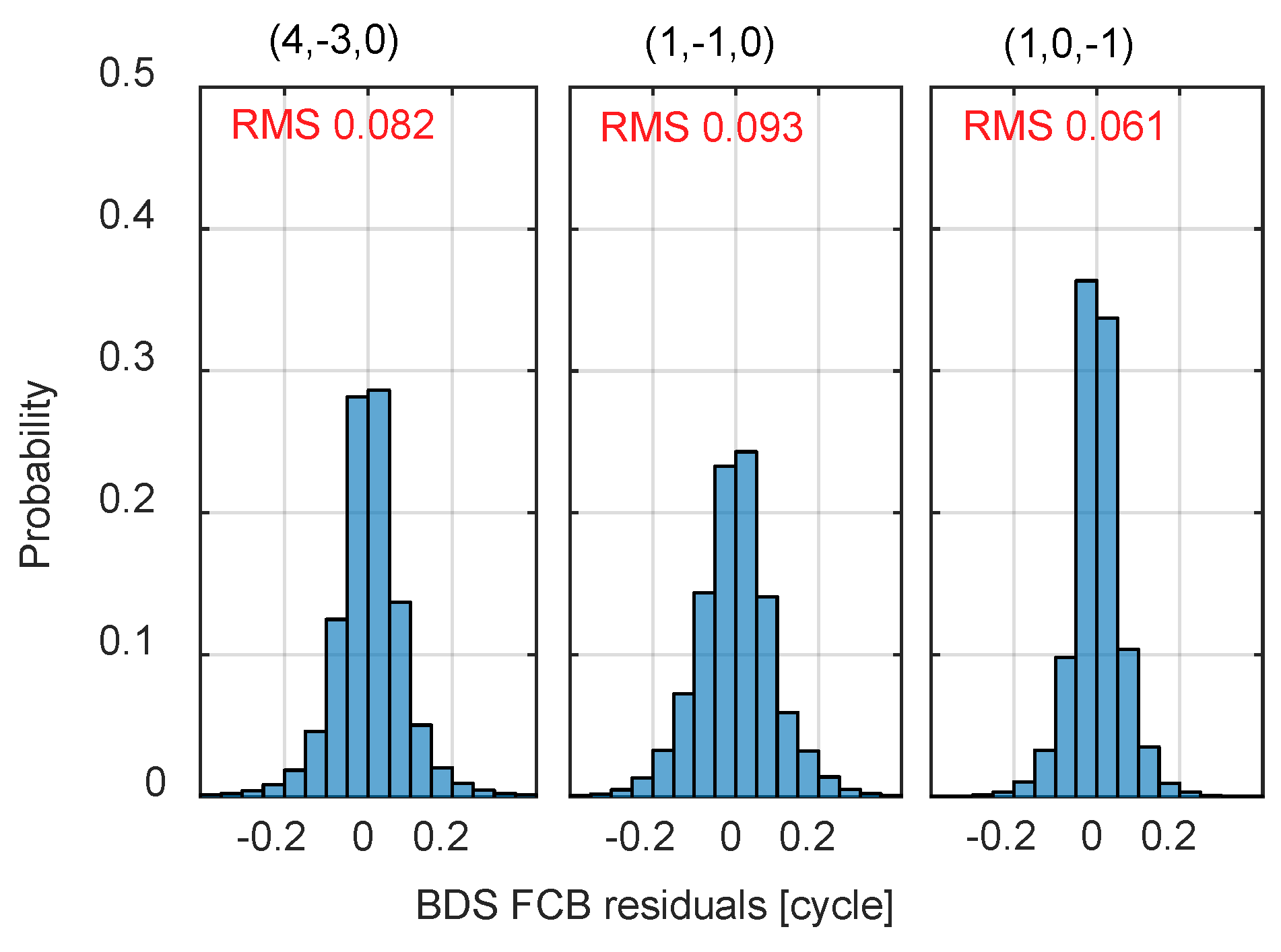
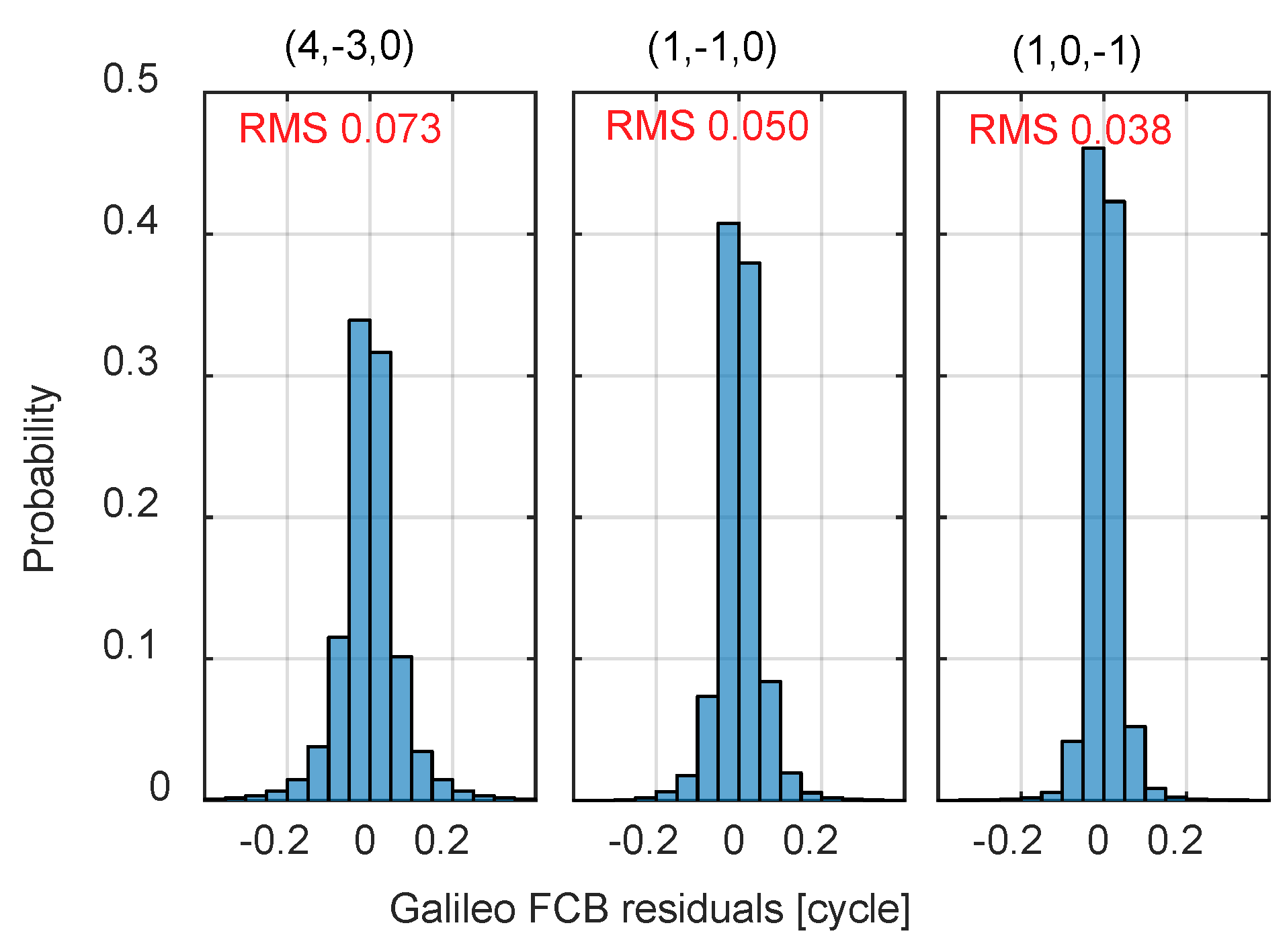
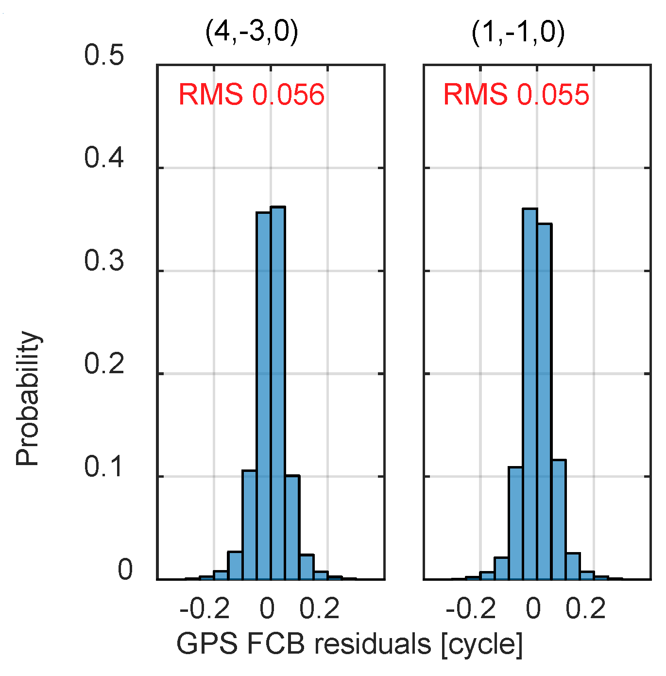
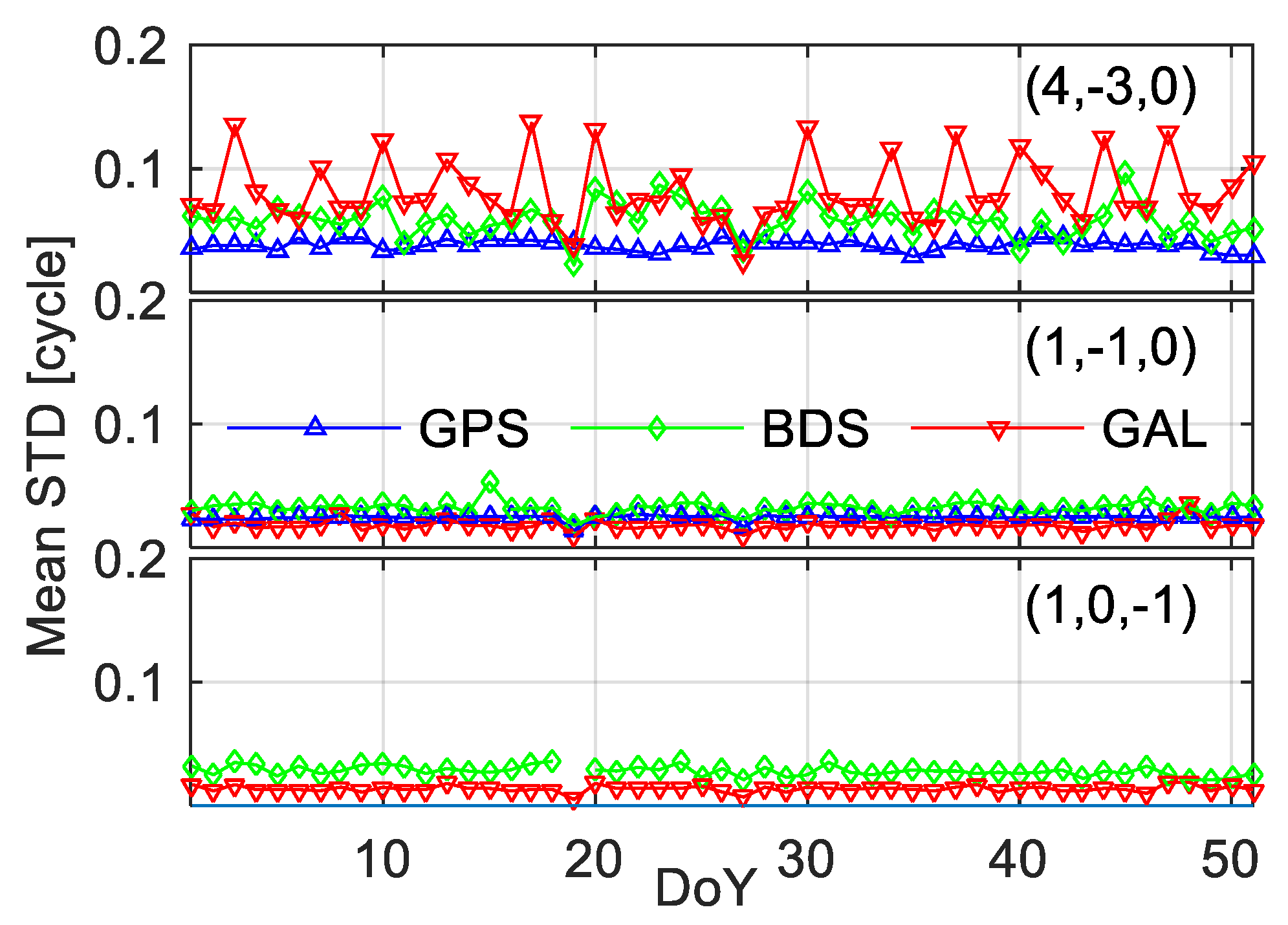
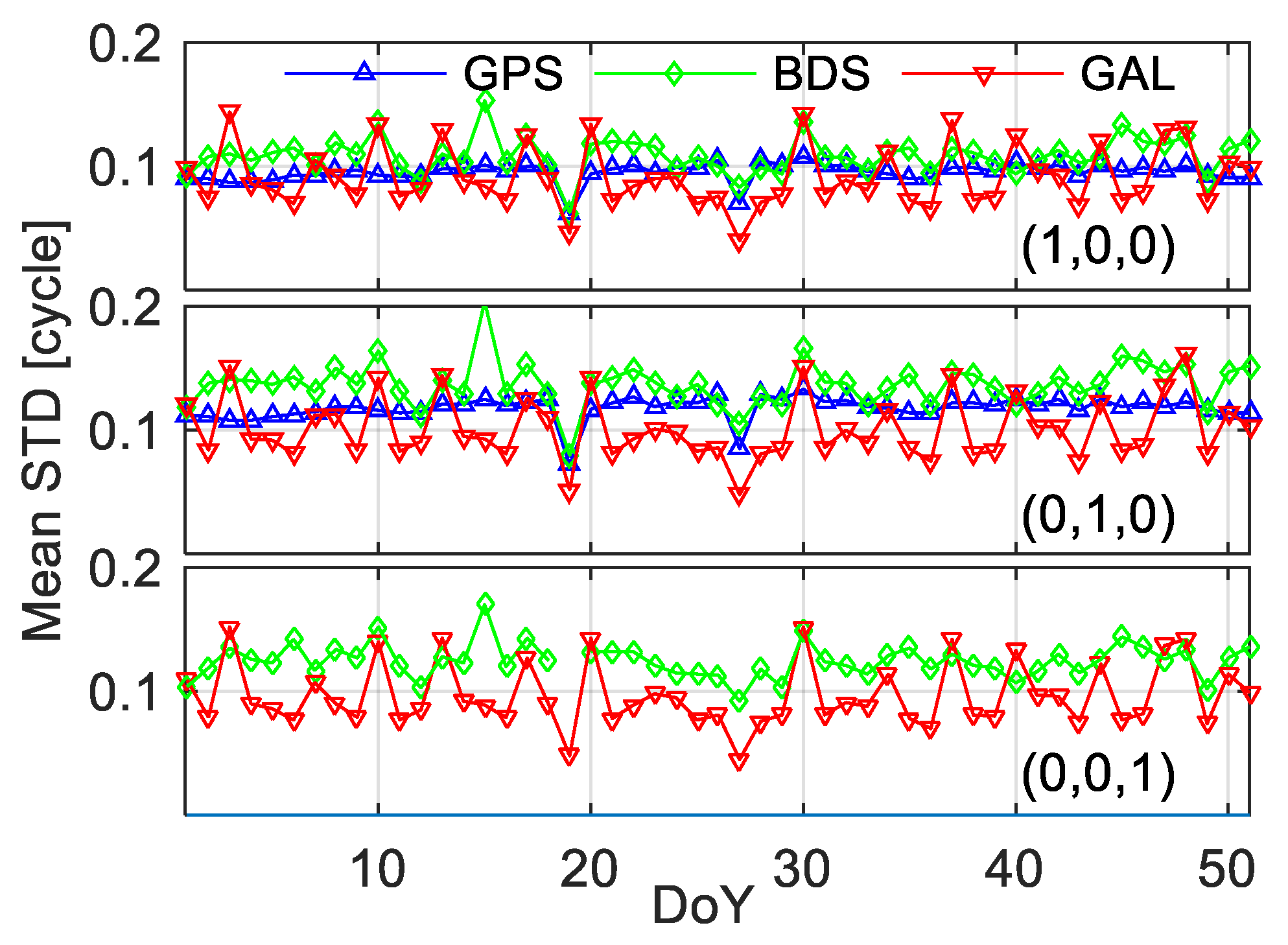
3.2. FCB Residual Distributions

The performance of PPP AR depends on the quality of the FCBs, which can be indicated by the posterior residuals. In general, a highly consistent FCB estimation can be expected if the residuals are close to zero. Figure 2, Figure 3 and Figure 4 present the distributions of the posterior residuals after FCB estimation for Galileo, BDS, and GPS, respectively. The subfigures refer to the different linear combinations.

In general, all the histograms are symmetric and nearly centered at zero, following Gaussian distributions. These results indicate a good consistency between the input float ambiguities and the generated FCBs, which prove the efficiency of the proposed FCB estimation strategy. However, the characteristics of residuals differ with respect to the combinations and systems.

For all the systems, the residuals of linear combinations with larger wavelengths are smaller. For example, the residuals of the NL combination with wavelength of around 10 cm, are larger than those of the other two combinations, i.e., WL/EWL. The reason is that the combination with smaller wavelength is susceptible to errors. An exception is that the BDS WL residuals are larger than that of NL. The reason is not clear, and we suspect that it may be related to the satellite induced multipath effect [39].

When comparing the residuals from multi-GNSS, it is found that the Galileo WL/EWL outperformed those of GPS and BDS. As discussed in Xiao, Li, Sui, Heck, and Schuh [21], the signal of Galileo possesses a better performance of multipath suppression, which may explain the results. For the NL, the residuals of GPS are the smallest, which is reasonable as the accuracy of the GPS PPP float solution is the highest.

Furthermore, the results are also different from that of IF PPP, in which the performance of WL is worse than that of the NL. The residuals of WL/NL in the uncombined PPP model are almost comparable in terms of root mean square (RMS) and distributions. The possible reason is that the WL ambiguities are directly formed from raw ambiguities in uncombined PPP, while it is derived from MW combinations in IF PPP. The noise of MW combinations is larger as code measurements are employed. In addition, the sample rate of WL FCB is 15 min in uncombined PPP, while that of IF PPP is 24 h. The larger sample interval may also increase the residuals.

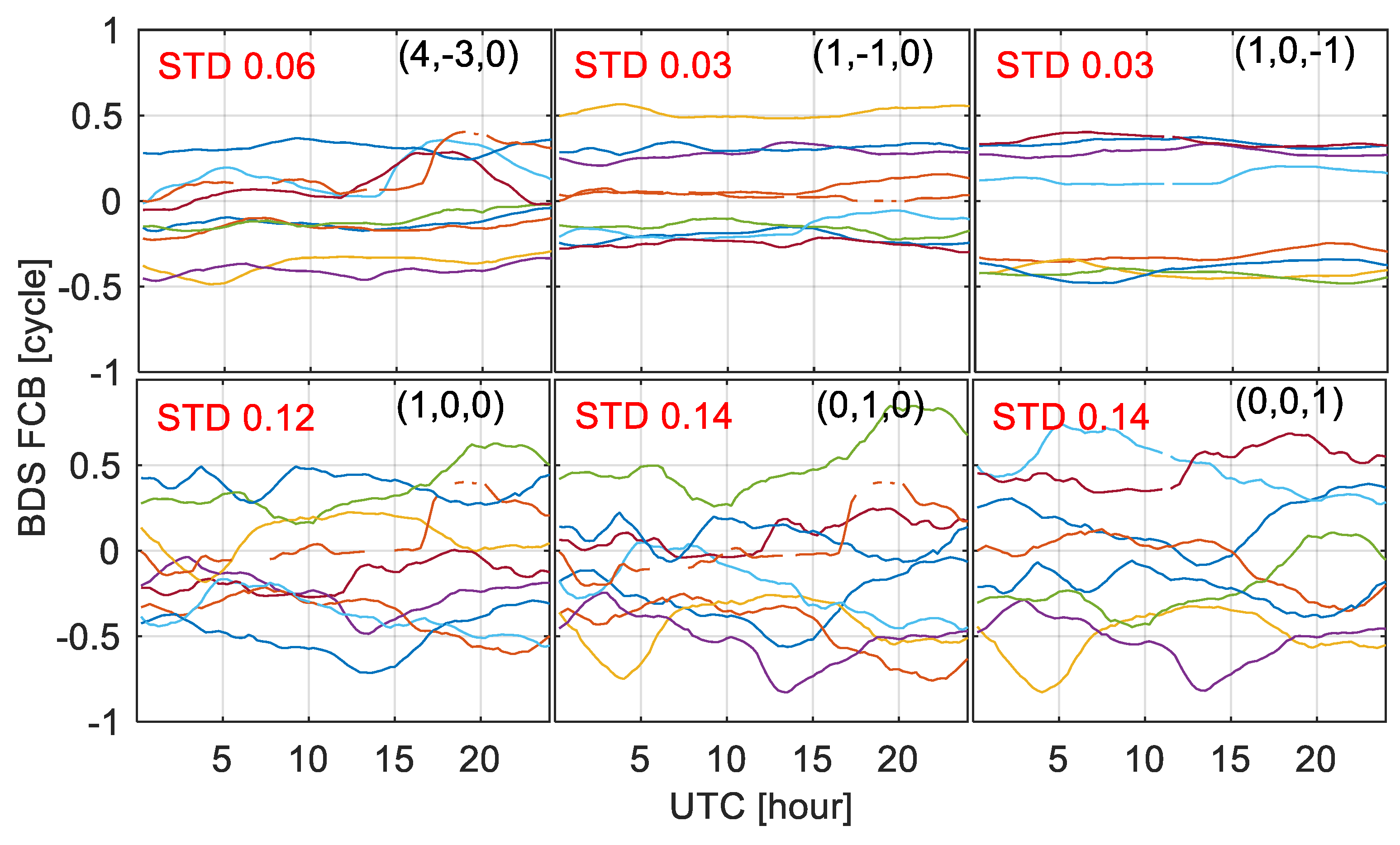
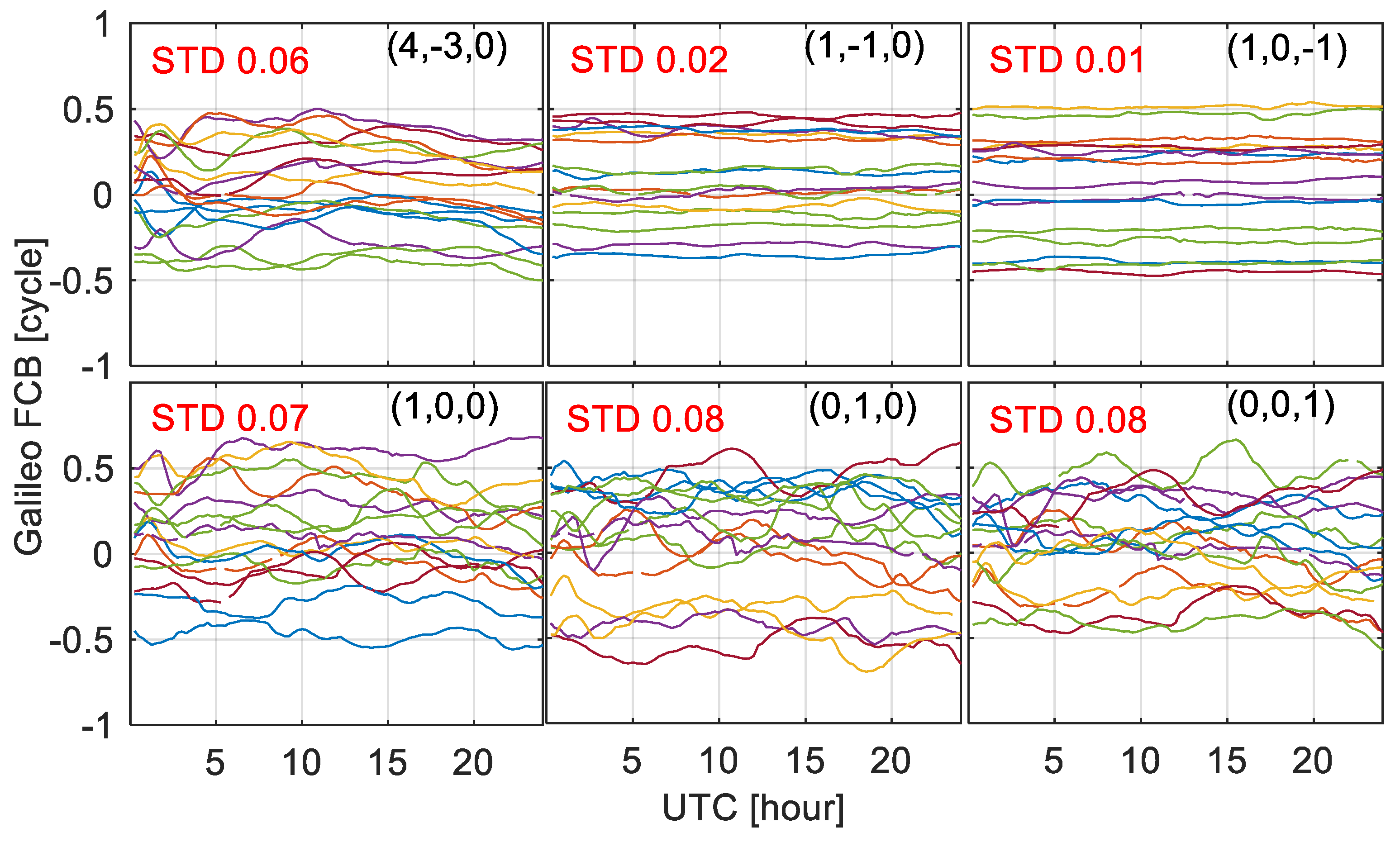
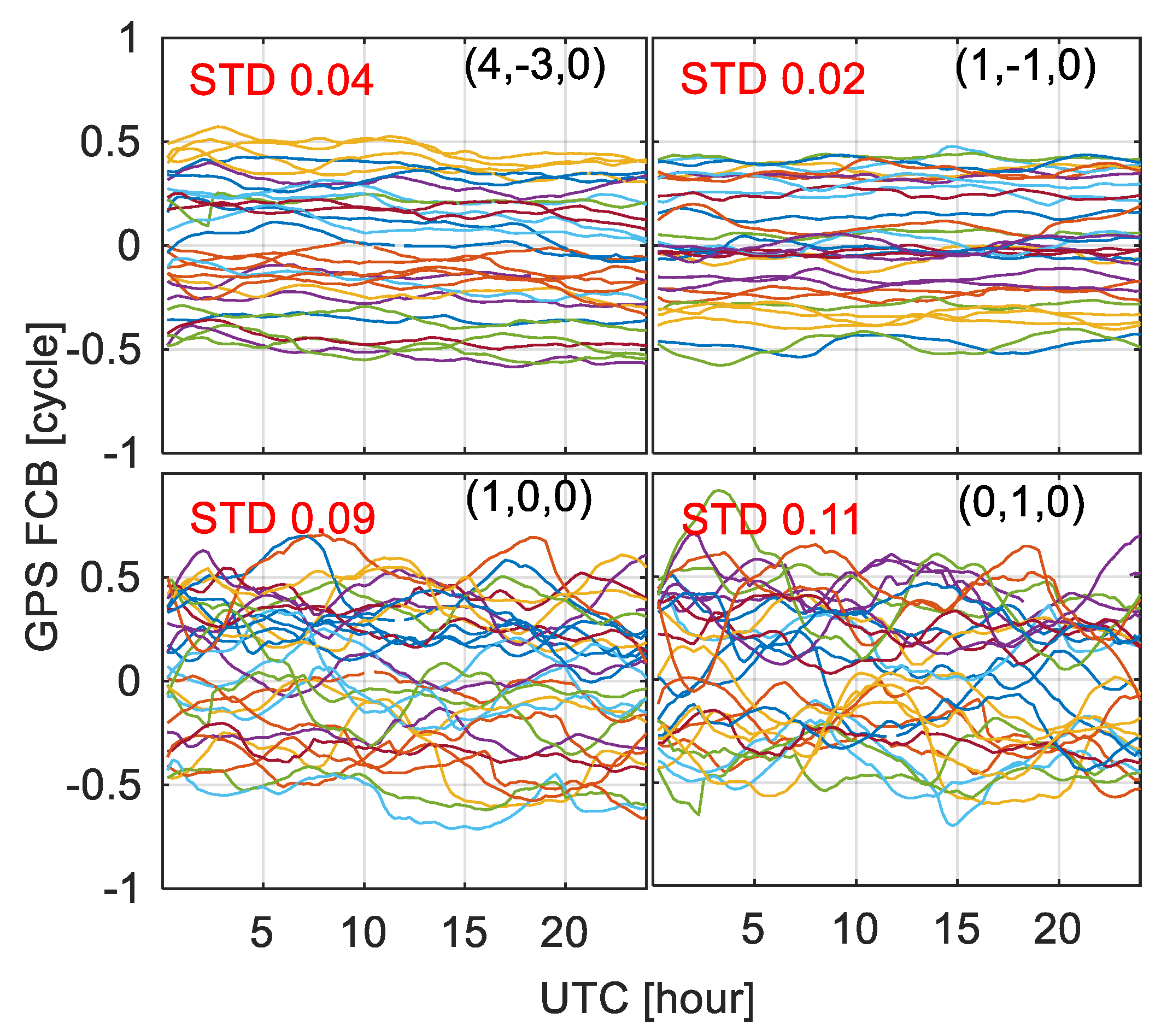
3.3. FCB Time Series

For real time applications, another question of interest is the temporal stability of the FCB estimates. It would be possible to predict the FCB if they are stable over time. Figure 5, Figure 6 and Figure 7 present the time series of FCBs for Galileo, BDS, and GPS, respectively.

In general, all the time series of FCB are quite stable over time. The fluctuations between adjacent sessions are smaller than 0.05 cycles, which indicates that the 15 min interval is sufficient for FCB estimation. When comparing the results from different linear combinations, it is found that the time series of NL FCB are noisier than those of WL/EWL FCB. The NL FCBs, possessing a smaller wavelength of about 10 cm, are susceptible to errors. The EWL shows extremely small variations over time, with a standard deviation of 0.01 cycles, as presented in Figure 8. For all the three systems, the raw FCBs are much noisier than that of the combined FCB (Figure 9). The raw FCBs, also having smaller wavelengths around 20 cm, are susceptible to ionospheric residuals, while it is eliminated or decreased by linear combinations in combined FCB. The average STD of combined FCB is around 0.03 cycles, while that for raw FCB is around 0.10 cycles. It is easier to predict the combined FCB, especially for the EWL/WL FCB. A lower update rate could be used to reduce the burden of communication. In this manner, it would be more efficient to broadcast combined FCB for real time applications.

When comparing the results from multi-GNSS, it can be seen that the STDs of Galileo EWL/WL FCBs are smaller than those of GPS and BDS, while that of the Galileo NL FCB is worse than GPS and BDS. The better quality of Galileo EWL/WL FCBs is likely attributed to the multipath suppression of Galileo signals, while the worse quality of Galileo NL FCB is due to the poor precision of satellite orbit and clock product. From Figure 9, it is found that the STDs of Galileo raw FCBs are smaller than that of GPS and BDS, regardless of combinations for most of the days. The smaller STDs facilitate the prediction of FCBs, which indicates a promising future for real time applications.

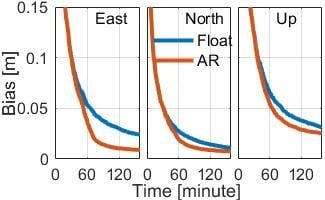
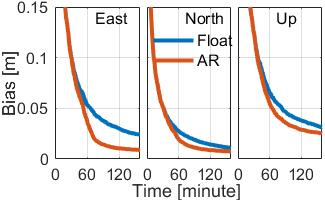
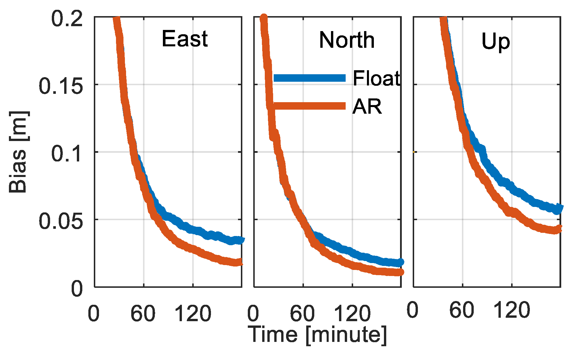
3.4. Triple-Frequency PPP AR

In order to validate our FCB estimates, as well as to assess the performance of triple-frequency PPP AR, 11 days from DoY 250 to 260 in 2017 of MGEX network stations are processed in static PPP AR mode. The 24 h observations are divided into eight three-hour sessions. The positional biases of BDS-only and Galileo-only PPP float solutions and AR solutions are presented in Figure 10 and Figure 11. The positional biases are calculated with respect to the 24-h static GPS/Galileo/BDS combined PPP solutions. The statistics of all the sessions in the 11 days are provided in

Table 2. Accuracy comparison of Galileo and BDS triple-frequency float and AR solutions (unit: cm).

System	No.	Solution	East	North	Up
BDS	804	float	3.70	1.83	6.12
		AR	1.88	1.13	4.31
		Improv.	49.2%	38.3%	29.6%
Galileo	5805	float	2.15	1.00	2.99
		AR	0.86	0.71	2.36
		Improv.	60.0%	29.0%	21.1%

. Note that the number of sessions for BDS is smaller than that of Galileo due to the regional BDS IGSO/MEO constellation.

It can be seen that the convergence time is significantly shortened by ambiguity resolution, especially for the east component. For Galileo triple-frequency observations, it takes 64.5 min for float solutions to converge to three-dimensional 10 cm accuracy, while that for AR solutions is only 56.0 min, corresponding to an improvement of 13.2%. For BDS triple-frequency observations, the corresponding numbers are 121.5 min, 97.0 min, and 20.2%, respectively. In addition, it can be seen that with the current constellation, the performance of Galileo already outperforms that of BDS, both in terms of float PPP and PPP AR.

From Table 2, it can be seen that PPP ambiguity resolution was able to enhance the accuracy for all the three components. The improvements of (east, north, up) components for positioning with BDS are (49.2%, 38.3%, and 29.6%), while that for positioning with Galileo are (60.0%, 29.0%, and 21.1%). The performance of BDS is worse than that of Galileo for both float and AR solutions. The worse performance of the BDS solution is likely ascribed to the incomplete convergence, which is due to the IGSO/MEO constellation and the limited number of observable satellites.

The additional signals are expected to further enhance the performance of PPP AR, as has been discussed in previous research [36,38,53]. Therefore, we also conduct an experiment to investigate the benefit of the third frequency observations in addition to dual-frequency ones. The strategy is that the ambiguities of the dual-frequency observations, i.e., B1/B2 and E1/E5a, are resolved to integers, while the ambiguities from the third frequency observations are kept as float values. This is accomplished by deleting the third column and row of the matrix in Equation (10). Then the results are compared to that of resolving the ambiguities of all the three-carrier frequencies. It is found that the improvements of positional error and convergence time are minimal. The positional improvements for Galileo are 1.8%, 2.3%, and 1.7%, while that of BDS are 8.0%, 5.0%, and 7.8%, for east, north, and up components, respectively. The possible reason could be: (1) the third frequency observations coming from the same satellites as the dual-frequency observations, will not improve the geometry of satellites, i.e., the DOP value. Compared with new observations from new satellites or other GNSS, its contribution to the model strength is insignificant; (2) the third carrier frequency E5b of Galileo is very close to the second one E5a, which implies the contribution of E5b is almost negligible when E1/E5a WL ambiguities are resolved. For BDS, the contribution of B3 is slightly larger than that of E5b, as its carrier frequency difference with respect to the B2 is larger; (3) the third frequency observations have been down-weighted due to lack of antenna corrections, which may also degrade the contribution of the third frequency.

4. Conclusions

A unified model for multi-frequency PPP AR based on raw uncombined observations is proposed, which simplifies the concept of phase biases for AR. No assumption is made on the method used to determine FCB on the server end, which implies that the generated FCB from multi-frequency observations could be flexibly used, such as for dual- or triple-frequency ones. It is demonstrated that the model is extendable to dual- and triple-frequency observations.

To verify its efficiency, we processed 51 days of Galileo and BDS triple-frequency observations collected from globally distributed MGEX stations. The estimated FCB shows a good consistency with the input float ambiguities. The RMS of Galileo FCB residuals is 0.05 cycles, while that of BDS is 0.08 cycles. It is also observed that the residuals are smaller for the combinations with larger wavelengths. The results indicate that there may exist ionospheric errors, and combinations are required to reduce its influence. The average STD of combined FCB is around 0.03 cycles, while that for raw FCB is around 0.10 cycles. To reduce the communication with servers for real time applications, it would be more efficient to broadcast linear combined FCB. The performance of triple-frequency PPP AR is assessed with 11 days of data in three-hour sessions. Compared with the float solutions, the positional biases of AR solutions are significantly improved. The improvements of ENU components for positioning with BDS are 49.2%, 38.3%, and 29.6%, while those for positioning with Galileo are 60.0%, 29.0%, and 21.1%. These results demonstrate the efficiency of the proposed FCB estimation approach, and that the triple-frequency PPP AR can bring an obvious benefit to the float solution.

When comparing triple-frequency PPP AR with that of dual-frequency, it is found that the contribution of the third frequency observations is minimal. The insignificant improvement of the third frequency observable may be due to its limited contribution to satellite geometry and the narrow deployment with respect to the second carrier frequency. Nevertheless, adding the third frequency increases the reliability since it is observed that the number of successful sessions is increased. The proposed model is also applicable to GPS triple-frequency observations, provided that the inter-frequency clock biases are accounted for, which will be investigated in the future.

References

1. Kouba, J.; Héroux, P. Precise Point Positioning Using IGS Orbit and Clock Products. GPS Solut. 2001, 5, 12–28. [Google Scholar] [CrossRef]
2. Zumberge, J.F.; Heflin, M.B.; Jefferson, D.C.; Watkins, M.M.; Webb, F.H. Precise point positioning for the efficient and robust analysis of GPS data from large networks. J. Geophys. Res. Solid Earth 1997, 102, 5005–5017. [Google Scholar] [CrossRef] [Green Version]
3. Cai, C.; Gao, Y.; Pan, L.; Zhu, J. Precise point positioning with quad-constellations: GPS, BeiDou, GLONASS and Galileo. Adv. Space Res. 2015, 56, 133–143. [Google Scholar] [CrossRef]
4. Gabor, M.J.; Nerem, R.S. GPS carrier phase AR using satellite-satellite single difference. In Proceedings of the 12th International Technical Meeting of the Satellite Division of The Institute of Navigation (ION GPS 1999), Nashville, TN, USA, 14–17 September 1999; pp. 1569–1578. [Google Scholar]
5. Gao, Y.; Shen, X. A new method for carrier-phase-based precise point positioning. Navigation 2002, 49, 109–116. [Google Scholar] [CrossRef]
6. Katsigianni, G.; Loyer, S.; Perosanz, F.; Mercier, F.; Zajdel, R.; Sośnica, K. Improving Galileo orbit determination using zero-difference ambiguity fixing in a Multi-GNSS processing. Adv. Space Res. 2018. [Google Scholar] [CrossRef]
7. Ge, M.; Gendt, G.; Rothacher, M.a.; Shi, C.; Liu, J. Resolution of GPS carrier-phase ambiguities in precise point positioning (PPP) with daily observations. J. Geod. 2008, 82, 389–399. [Google Scholar] [CrossRef]
8. Li, P.; Zhang, X.; Ren, X.; Zuo, X.; Pan, Y. Generating GPS satellite fractional cycle bias for ambiguity-fixed precise point positioning. GPS Solut. 2015, 20, 771–782. [Google Scholar] [CrossRef]
9. Xiao, G.; Sui, L.; Heck, B.; Zeng, T.; Tian, Y. Estimating satellite phase fractional cycle biases based on Kalman filter. GPS Solut. 2018, 22, 82. [Google Scholar] [CrossRef]
10. Collins, P.; Lahaye, F.; Héroux, P.; Bisnath, S. Precise point positioning with ambiguity resolution using the decoupled clock model. In Proceedings of the 21st International Technical Meeting of the Satellite Division of The Institute of Navigation (ION GNSS 2008), Savannah, Georgia, 16–19 September 2008; pp. 1315–1322. [Google Scholar]
11. Laurichesse, D.; Mercier, F.; Berthias, J.-P.; Broca, P.; Cerri, L. Integer ambiguity resolution on undifferenced GPS phase measurements and its application to PPP and satellite precise orbit determination. Navigation 2009, 56, 135–149. [Google Scholar] [CrossRef]
12. Shi, J.; Gao, Y. A comparison of three PPP integer ambiguity resolution methods. GPS Solut. 2014, 18, 519–528. [Google Scholar] [CrossRef]
13. Teunissen, P.J.G.; Khodabandeh, A. Review and principles of PPP-RTK methods. J. Geod. 2015, 89, 217–240. [Google Scholar] [CrossRef]
14. Geng, J.; Meng, X.; Dodson, A.H.; Teferle, F.N. Integer ambiguity resolution in precise point positioning: Method comparison. J. Geod. 2010, 84, 569–581. [Google Scholar] [CrossRef]
15. Geng, J.; Shi, C. Rapid initialization of real-time PPP by resolving undifferenced GPS and GLONASS ambiguities simultaneously. J. Geod. 2016, 91, 361–374. [Google Scholar] [CrossRef]
16. Yi, W.; Song, W.; Lou, Y.; Shi, C.; Yao, Y.; Guo, H.; Chen, M.; Wu, J. Improved method to estimate undifferenced satellite fractional cycle biases using network observations to support PPP ambiguity resolution. GPS Solut. 2017, 21, 1369–1378. [Google Scholar] [CrossRef]
17. Liu, Y.; Ye, S.; Song, W.; Lou, Y.; Gu, S. Rapid PPP ambiguity resolution using GPS+ GLONASS observations. J. Geod. 2017, 91, 441–455. [Google Scholar] [CrossRef]
18. Li, P.; Zhang, X.; Guo, F. Ambiguity resolved precise point positioning with GPS and BeiDou. J. Geod. 2017, 91, 25–40. [Google Scholar]
19. Liu, Y.; Ye, S.; Song, W.; Lou, Y.; Chen, D. Integrating GPS and BDS to shorten the initialization time for ambiguity-fixed PPP. GPS Solut. 2017, 21, 333–343. [Google Scholar] [CrossRef]
20. Tegedor, J.; Liu, X.; Jong, K.; Goode, M.; Øvstedal, O.; Vigen, E. Estimation of Galileo Uncalibrated Hardware Delays for Ambiguity-Fixed Precise Point Positioning. Navigation 2016, 63, 173–179. [Google Scholar] [CrossRef]
21. Xiao, G.; Li, P.; Sui, L.; Heck, B.; Schuh, H. Estimating and assessing Galileo satellite fractional cycle bias for PPP ambiguity resolution. GPS Solut. 2019, 23. [Google Scholar] [CrossRef]
22. Li, X.; Li, X.; Yuan, Y.; Zhang, K.; Zhang, X.; Wickert, J. Multi-GNSS phase delay estimation and PPP ambiguity resolution: GPS, BDS, GLONASS, Galileo. J. Geod. 2017, 92, 579–608. [Google Scholar] [CrossRef]
23. Montenbruck, O.; Steigenberger, P.; Prange, L.; Deng, Z.; Zhao, Q.; Perosanz, F.; Romero, I.; Noll, C.; Sturze, A.; Weber, G.; et al. The multi-GNSS experiment (MGEX) of the international GNSS service (IGS)—Achievements, prospects and challenges. Adv. Space Res. 2017, 59, 1671–1697. [Google Scholar] [CrossRef]
24. Schönemann, E.; Becker, M.; Springer, T. A new approach for GNSS analysis in a multi-GNSS and multi-signal environment. J. Geod. Sci. 2011, 1, 204–214. [Google Scholar] [CrossRef]
25. Gu, S.; Shi, C.; Lou, Y.; Liu, J. Ionospheric effects in uncalibrated phase delay estimation and ambiguity-fixed PPP based on raw observable model. J. Geod. 2015, 89, 447–457. [Google Scholar] [CrossRef]
26. Lou, Y.; Zheng, F.; Gu, S.; Wang, C.; Guo, H.; Feng, Y. Multi-GNSS precise point positioning with raw single-frequency and dual-frequency measurement models. GPS Solut. 2016, 20, 849–862. [Google Scholar] [CrossRef]
27. Chen, J.; Zhang, Y.; Wang, J.; Yang, S.; Dong, D.; Wang, J.; Qu, W.; Wu, B. A simplified and unified model of multi-GNSS precise point positioning. Adv. Space Res. 2015, 55, 125–134. [Google Scholar] [CrossRef]
28. Feng, Y.; Gu, S.; Shi, C.; Rizos, C. A reference station-based GNSS computing mode to support unified precise point positioning and real-time kinematic services. J. Geod. 2013, 87, 945–960. [Google Scholar] [CrossRef]
29. Odijk, D.; Zhang, B.; Khodabandeh, A.; Odolinski, R.; Teunissen, P.J.G. On the estimability of parameters in undifferenced, uncombined GNSS network and PPP-RTK user models by means of S system theory. J. Geod. 2016, 90, 15–44. [Google Scholar] [CrossRef]
30. Tu, R.; Zhang, H.; Ge, M.; Huang, G. A real-time ionospheric model based on GNSS Precise Point Positioning. Adv. Space Res. 2013, 52, 1125–1134. [Google Scholar] [CrossRef]
31. Zhang, B.; Ou, J.; Yuan, Y.; Li, Z. Extraction of line-of-sight ionospheric observables from GPS data using precise point positioning. Sci. China Earth Sci. 2012, 55, 1919–1928. [Google Scholar] [CrossRef]
32. Liu, T.; Zhang, B.; Yuan, Y.; Li, Z.; Wang, N. Multi-GNSS triple-frequency differential code bias (DCB) determination with precise point positioning (PPP). J. Geod. 2018, 1–20. [Google Scholar] [CrossRef]
33. Shi, C.; Fan, L.; Li, M.; Liu, Z.; Gu, S.; Zhong, S.; Song, W. An enhanced algorithm to estimate BDS satellite’s differential code biases. J. Geod. 2015, 90, 161–177. [Google Scholar] [CrossRef]
34. Zehentner, N.; Mayer-Gürr, T. Precise orbit determination based on raw GPS measurements. J. Geod. 2016, 90, 275–286. [Google Scholar] [CrossRef]
35. Guo, F.; Zhang, X.; Wang, J. Timing group delay and differential code bias corrections for BeiDou positioning. J. Geod. 2015, 89, 427–445. [Google Scholar] [CrossRef]
36. Li, P.; Zhang, X.; Ge, M.; Schuh, H. Three-frequency BDS precise point positioning ambiguity resolution based on raw observables. J. Geod. 2018, 92, 1357–1369. [Google Scholar] [CrossRef]
37. Li, X.; Ge, M.; Zhang, H.; Wickert, J. A method for improving uncalibrated phase delay estimation and ambiguity-fixing in real-time precise point positioning. J. Geod. 2013, 87, 405–416. [Google Scholar] [CrossRef]
38. Gu, S.; Lou, Y.; Shi, C.; Liu, J. BeiDou phase bias estimation and its application in precise point positioning with triple-frequency observable. J. Geod. 2015, 89, 979–992. [Google Scholar] [CrossRef]
39. Wanninger, L.; Beer, S. BeiDou satellite-induced code pseudorange variations: Diagnosis and therapy. GPS Solut. 2015, 19, 639–648. [Google Scholar] [CrossRef]
40. Wang, N.; Yuan, Y.; Li, Z.; Montenbruck, O.; Tan, B. Determination of differential code biases with multi-GNSS observations. J. Geod. 2016, 90, 209–228. [Google Scholar] [CrossRef]
41. Leick, A.; Rapoport, L.; Tatarnikov, D. GPS Satellite Surveying; John Wiley & Sons: Hoboken, NJ, USA, 2015. [Google Scholar]
42. Hadas, T.; Krypiak-Gregorczyk, A.; Hernández-Pajares, M.; Kaplon, J.; Paziewski, J.; Wielgosz, P.; Garcia-Rigo, A.; Kazmierski, K.; Sosnica, K.; Kwasniak, D.; et al. Impact and Implementation of Higher-Order Ionospheric Effects on Precise GNSS Applications: Higher-Order Ionospheric Effects in GNSS. J. Geophys. Res. Solid Earth 2017, 122, 9420–9436. [Google Scholar] [CrossRef]
43. Dach, R.; Lutz, S.; Walser, P.; Fridez, P. Bernese GNSS Software Version 5.2; University of Bern, Bern Open Publishing: Bern, Switzerland, 2015. [Google Scholar]
44. Teunissen, P.J.G.; Jonge, P.J.; Tiberius, C.C.J.M. Performance of the LAMBDA method for fast GPS ambiguity resolution. Navigation 1997, 44, 373–383. [Google Scholar] [CrossRef]
45. Weber, G.; Dettmering, D.; Gebhard, H. Networked Transport of RTCM via Internet Protocol (NTRIP). In Proceedings of the A Window on the future on Geodesy, Sapporo, Japan, 30 June–11 July 2003; pp. 60–64. [Google Scholar]
46. Teunissen, P.J.G.; Joosten, P.; Tiberius, C.C.J.M. Geometry-free ambiguity success rates in case of partial fixing. In Proceedings of the 1999 National Technical Meeting of The Institute of Navigation, San Diego, CA, USA, 25–27 January 1999; pp. 25–27. [Google Scholar]
47. Li, P.; Zhang, X. Precise point positioning with partial ambiguity fixing. Sensors 2015, 15, 13627–13643. [Google Scholar] [CrossRef] [PubMed]
48. Pan, L.; Zhang, X.; Guo, F.; Liu, J. GPS inter-frequency clock bias estimation for both uncombined and ionospheric-free combined triple-frequency precise point positioning. J. Geod. 2018, 1–15. [Google Scholar] [CrossRef]
49. Lei, W.; Wu, G.; Tao, X.; Bian, L.; Wang, X. BDS satellite-induced code multipath: Mitigation and assessment in new-generation IOV satellites. Adv. Space Res. 2017, 60, 2672–2679. [Google Scholar] [CrossRef]
50. Uhlemann, M.; Gendt, G.; Ramatschi, M.; Deng, Z. GFZ Global Multi-GNSS Network and Data Processing Results. In IAG 150 Years; Springer: Heidelberg, Germany, 2016; pp. 673–679. [Google Scholar]
51. Prange, L.; Orliac, E.; Dach, R.; Arnold, D.; Beutler, G.; Schaer, S.; Jäggi, A. CODE’s five-system orbit and clock solution—The challenges of multi-GNSS data analysis. J. Geod. 2017, 91, 345–360. [Google Scholar] [CrossRef]
52. Kazmierski, K.; Hadas, T.; Sośnica, K. Weighting of Multi-GNSS Observations in Real-Time Precise Point Positioning. Remote Sens. 2018, 10, 84. [Google Scholar] [CrossRef]
53. Geng, J.; Bock, Y. Triple-frequency GPS precise point positioning with rapid ambiguity resolution. J. Geod. 2013, 87, 449–460. [Google Scholar] [CrossRef]
Figure 1. Geographic distribution of the selected MGEX stations with Galileo (represented by empty circles) and BDS (represented by solid triangles) triple-frequency observations.
Remotesensing 11 00116 g001
Figure 2. Distributions of posterior residuals of Galileo FCB for different linear combinations.
Remotesensing 11 00116 g002
Figure 3. Distributions of posterior residuals of BDS FCB for different linear combinations.
Remotesensing 11 00116 g003
Figure 4. Distributions of posterior residuals of GPS FCB for different linear combinations.
Remotesensing 11 00116 g004
Figure 5. Time series of the combined (upper) and raw (bottom) Galileo FCB in each 15 min session on DoY 255, 2017.
Remotesensing 11 00116 g005
Figure 6. Time series of the combined (upper) and raw (bottom) BDS FCB in each 15 min session on DoY 255, 2017.
Remotesensing 11 00116 g006
Figure 7. Time series of the combined (upper) and raw (bottom) GPS FCB in each 15 min session on DoY 255, 2017.
Remotesensing 11 00116 g007
Figure 8. Mean STD of the combined FCB series for all the 51 days. Daily STD is calculated for each satellite FCB series. For each day, the mean STD of all satellite daily STDs is presented.
Remotesensing 11 00116 g008
Figure 9. Mean STD of the raw FCB series for all the 51 days. Daily STD is calculated for each satellite FCB series. For each day, the mean STD of all satellite daily STDs is presented.
Remotesensing 11 00116 g009
Figure 10. Convergence performance of BDS triple-frequency PPP float and AR solutions based on 804 3-h sessions under 68% confidence level.
Remotesensing 11 00116 g010
Figure 11. Convergence performance of Galileo triple-frequency PPP float and AR solutions based on 5805 3-h sessions under 68% confidence level.
Remotesensing 11 00116 g011