Methodology for Processing of 3D Multibeam Sonar Big Data for Comparative Navigation

 ,
,  , ,
, ,
Abstract
1. Introduction
- Determining the point of best match of the image with the pattern. The logical conjunction algorithm is used and it finds the point of best match of images recorded as a digital matrix. The comparison between the registered real image and the source image (in this case bENCs) as a whole is done using a method that can determine global difference or global similarity between the images.
- Using previously registered real images associated with the position of their registration. This method uses an artificial neural network (ANN) trained by a sequence created from vectors representing the compressed images and the corresponding position of the vehicle.
- Using the generated map of patterns. An ANN is trained with a representation of selected images corresponding to the potential positions of the vehicle. The patterns are generated based on a numerical terrain model, knowledge of the effect of the hydrometeorological conditions and the observation specificity of the selected device.
2. Materials and Methods
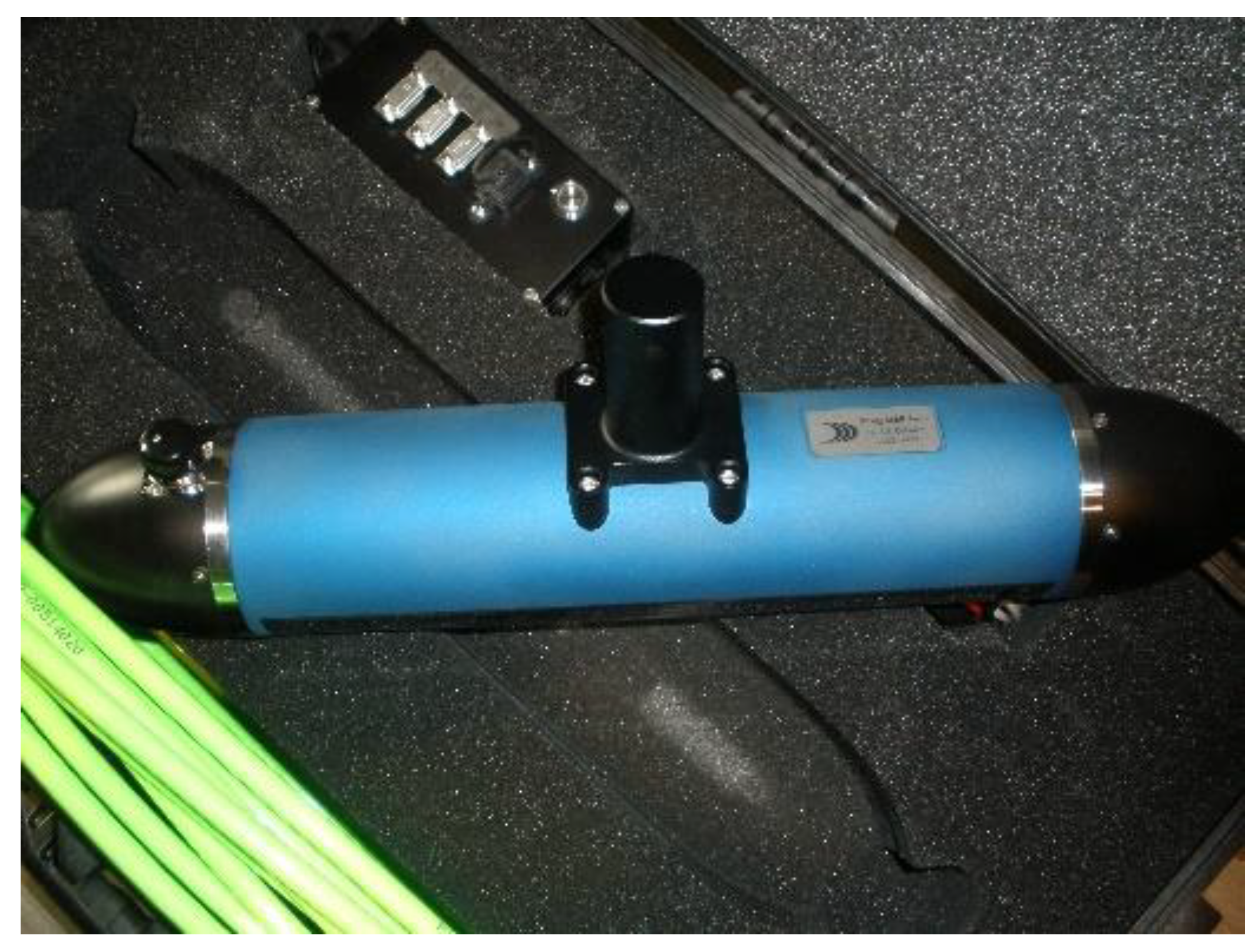
2.1. Instrument Description
2.2. Test Area Characteristics
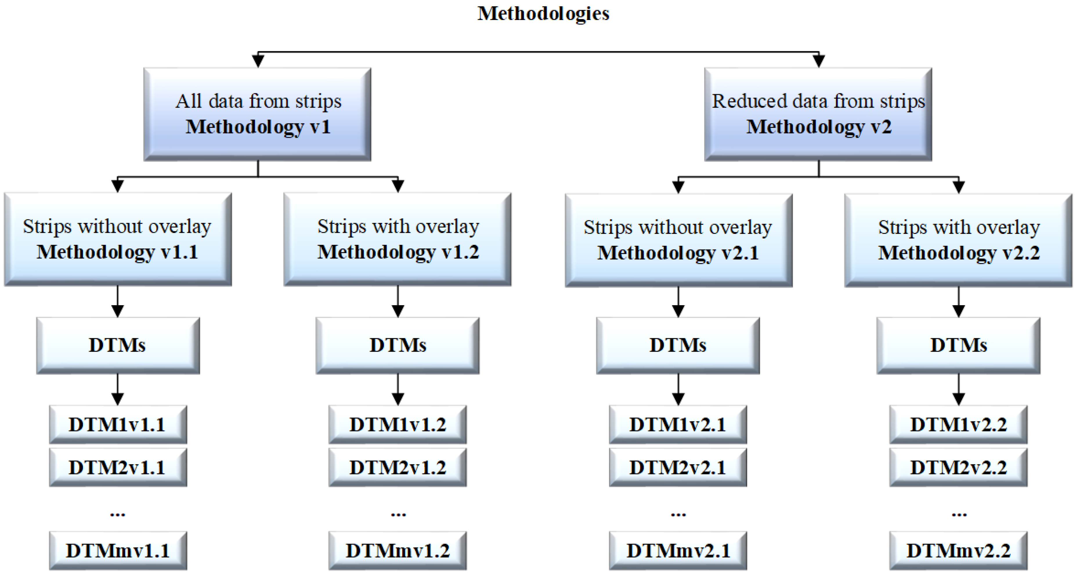
2.3. Methodology
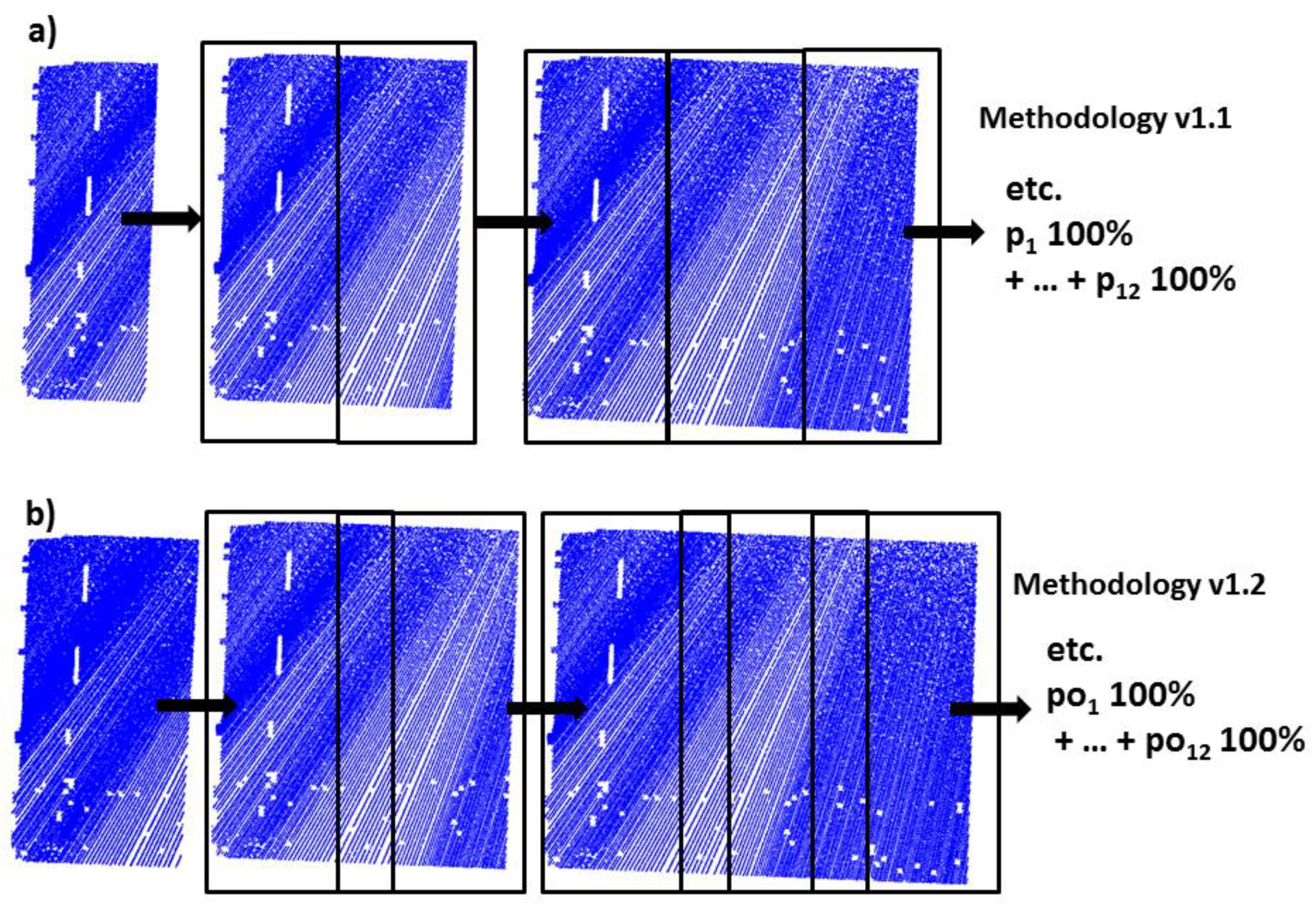
2.3.1. Methodology v1
- (a)
- The test area was divided into strips pi without overlay between them, where pi was a strip with observations, i= 1, 2, 3 …, m, and m was the number of strips.
- (b)
- The test area was divided into strips poi with 25–30% overlay between them, where poi was a strip with observations, i = 1, 2, 3 …, m, and m is the number of strips.
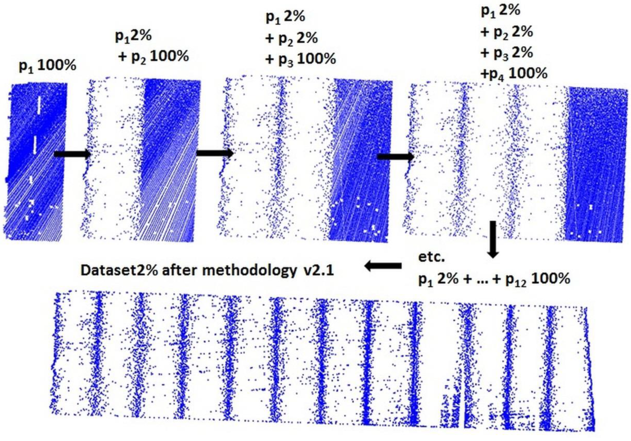
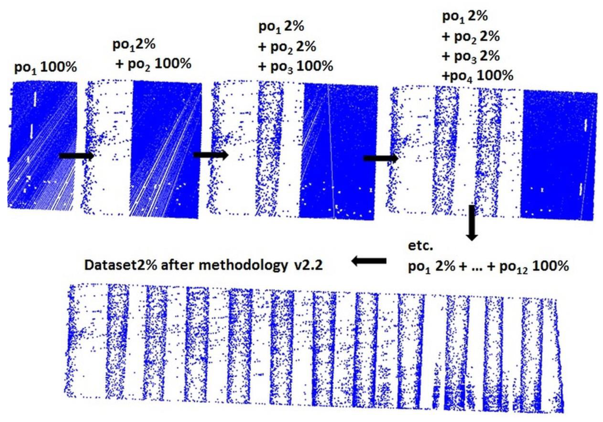
2.3.2. Methodology v2
- (a)
- The test area was divided into strips pi without overlay between them and the set was reduced by the OptD method.
- (b)
- The test area was divided into strips poi with 25–30% overlay between them and the set was reduced by the OptD method.
- (a)
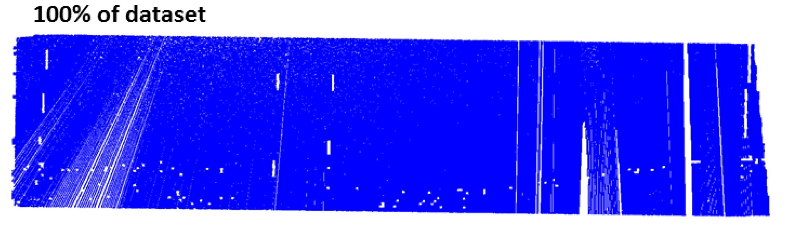
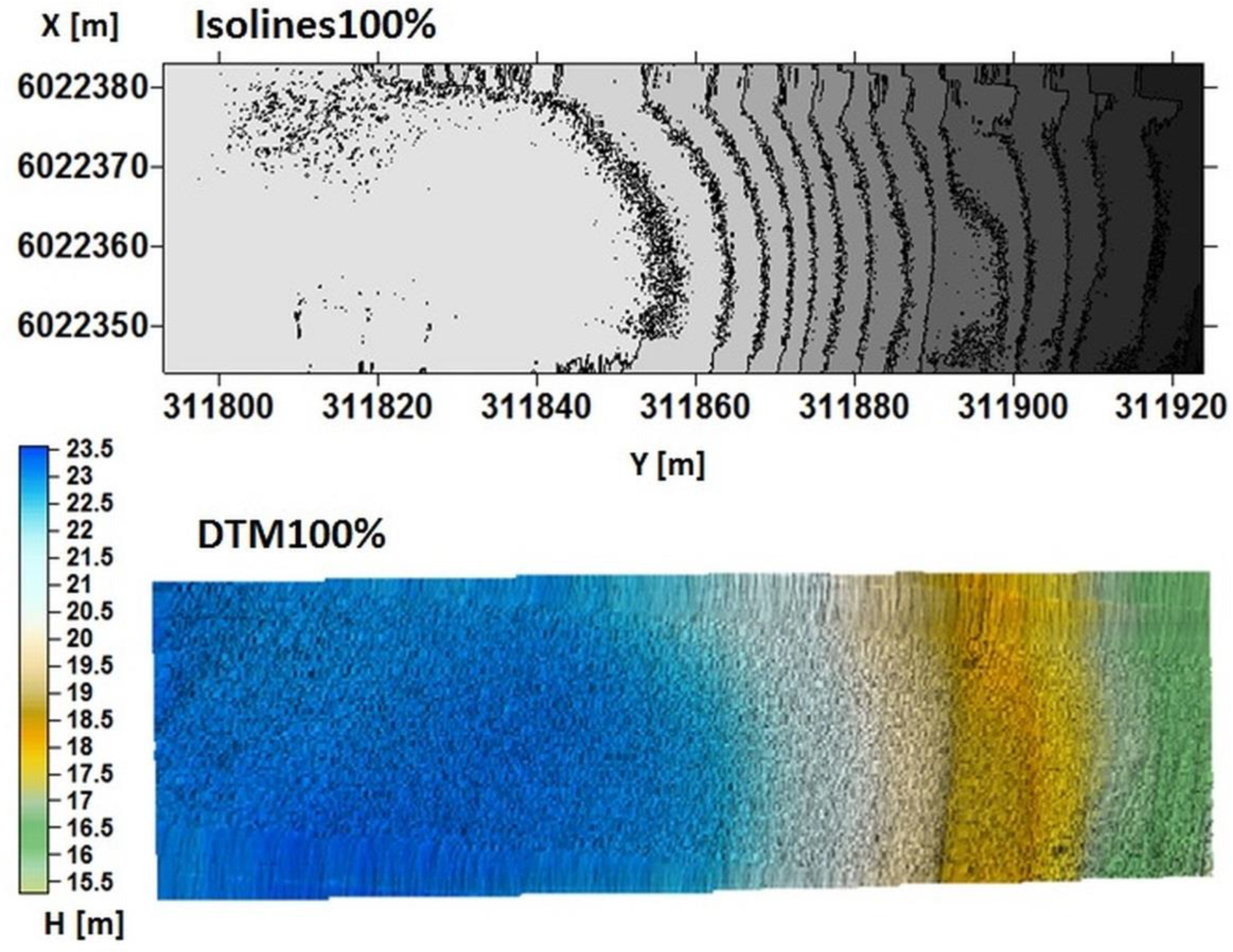
- DTM100% = whole DTMv1.1 = whole DTMv1.2.
- (b)
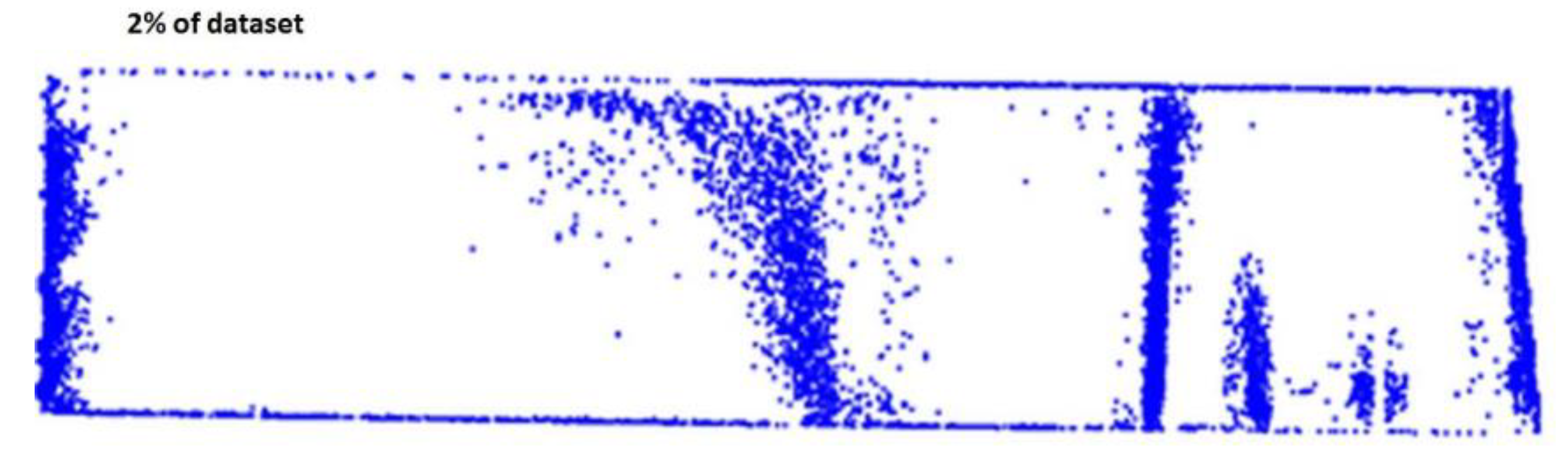
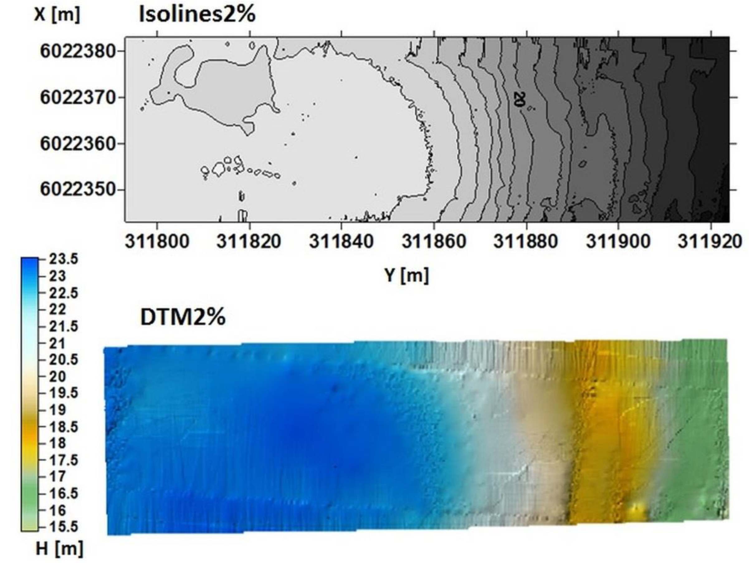
- DTM2% = whole DTMv2.1 = whole DTMv2.2.
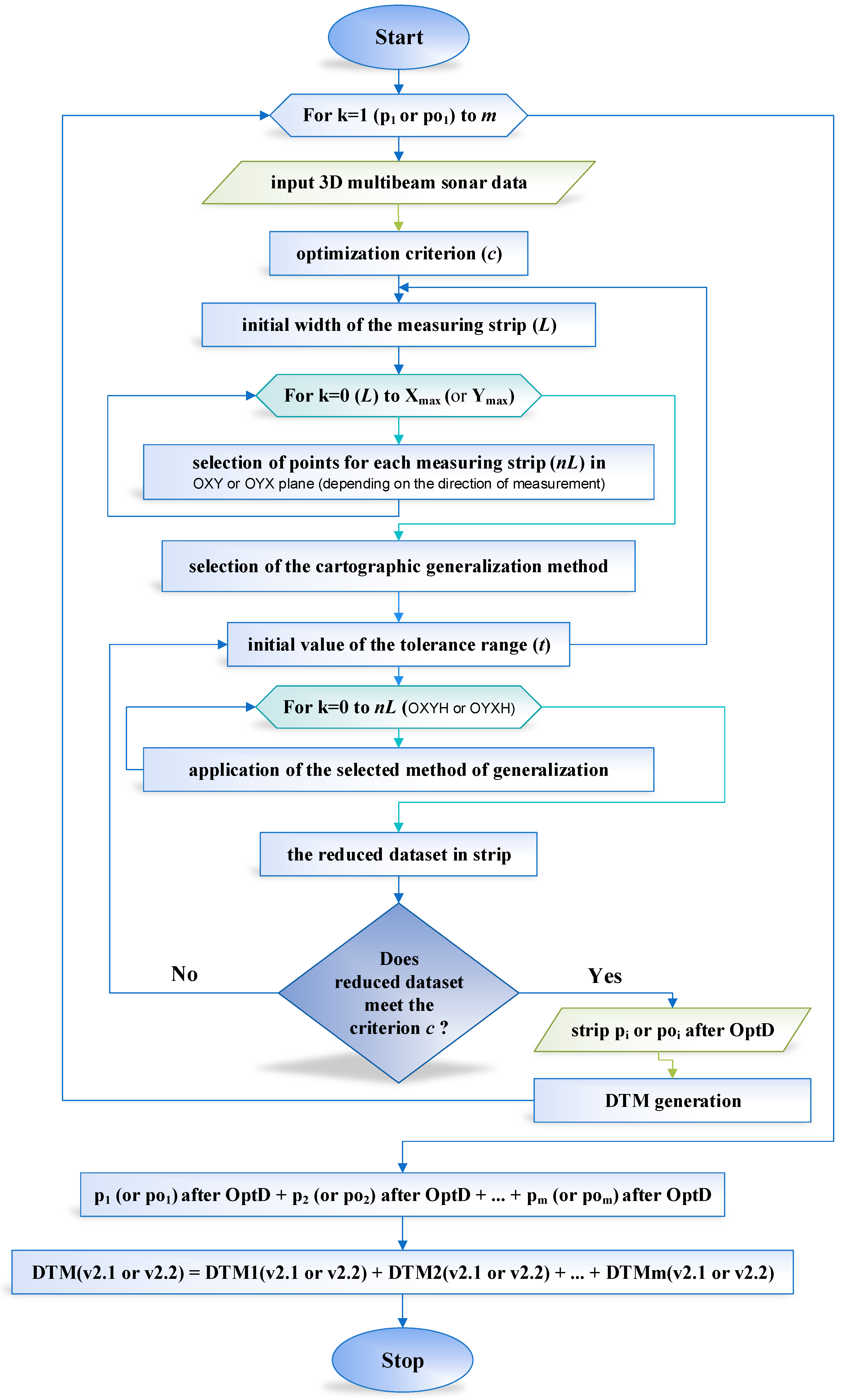
2.3.3. OptD method
- (a)
- For methodology v2.1, the whole dataset after reduction = p1 after OptD + p2 after OptD + … + pm after OptD
- (b)
- For methodology v2.2, the whole dataset after reduction = po1 after OptD + po2 after OptD + … + pom after OptD
- (a)
- For v2.1, the whole DTMv2.1 = DTM1v2.1 + DTM2v2.1 + … + DTMmv2.1
- (b)
- For v2.2, the whole DTMv2.2 = DTM1v2.2 + DTM2v2.2 + … + DTMmv2.2
2.3.4. Reduction
3. Results
4. Discussion
- The total generation time for DTMv1.1 was 159 s, whereas that for DTMv2.1 was 126 s.
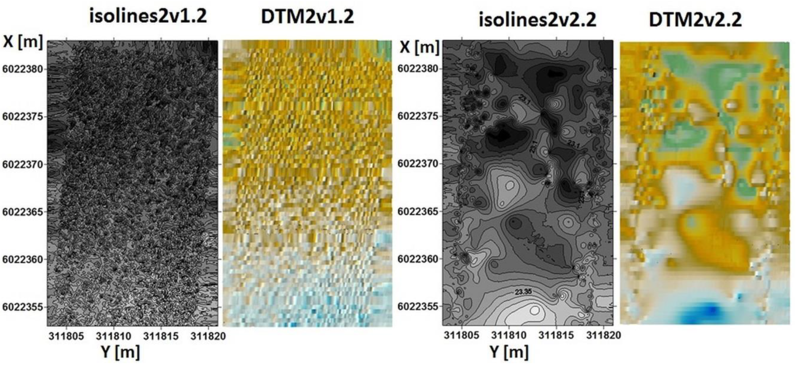
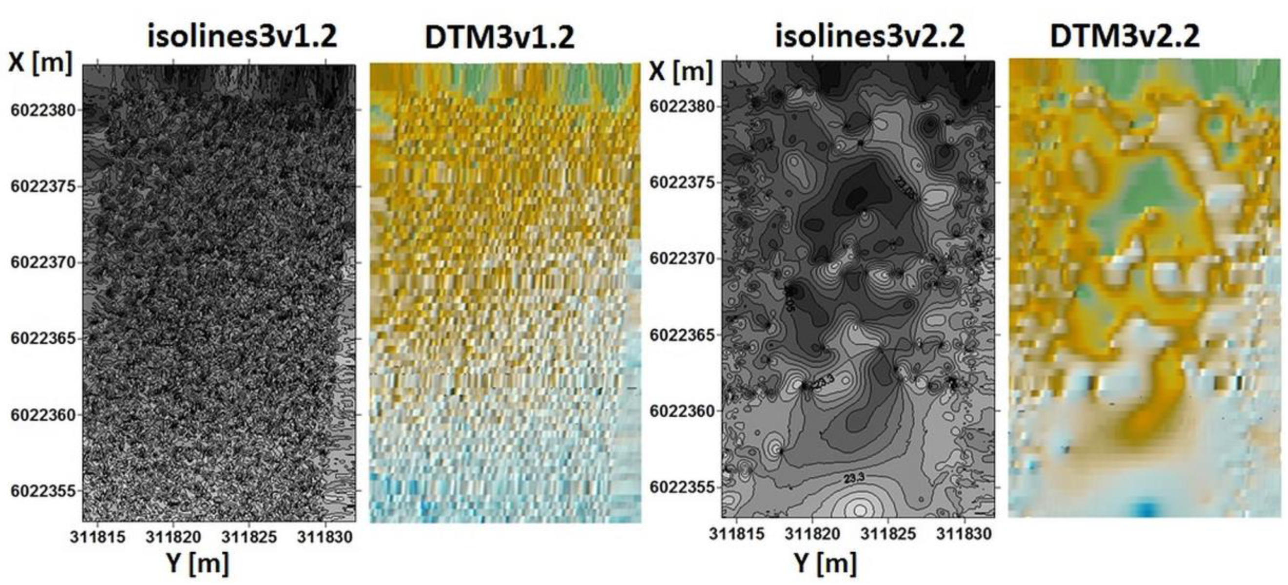
- The generation time for DTMv1.2 was 260 s, whereas that for DTMv2.2 was 201 s.
- The time needed for DTM generation was 268 s for DTM100% and 150 s for DTM2%.
5. Conclusions
- The new methodology is dedicated for 3D multibeam sonar data.
- The new approach consists of the following steps: Acquisition the fragment of data, reducing data, and 3D model generation.
- At the same time, the one fragment of data was processed with a new methodology, the next fragment of data was measured. This approach allows fast processing.
- The generated DTMs or isolines maps can be simultaneously compared with existing maps (for example bENCs).
- The time needed for fragmentary processing of 3D multibeam sonar data is shorter than the time needed for processing the whole data set.
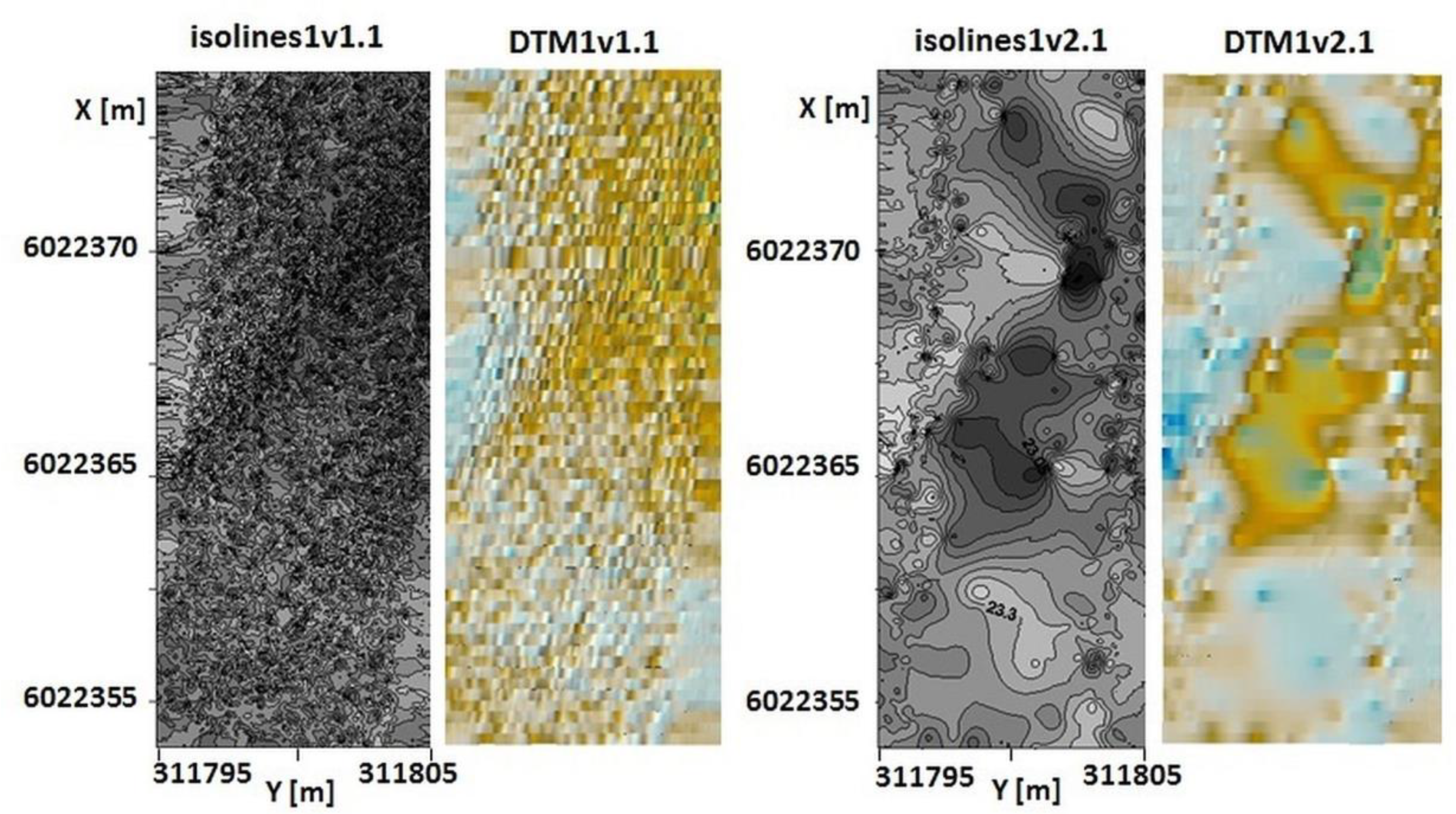
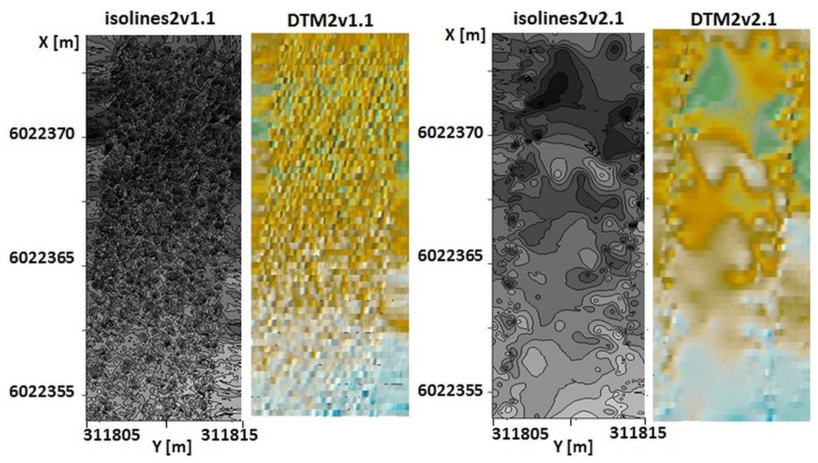
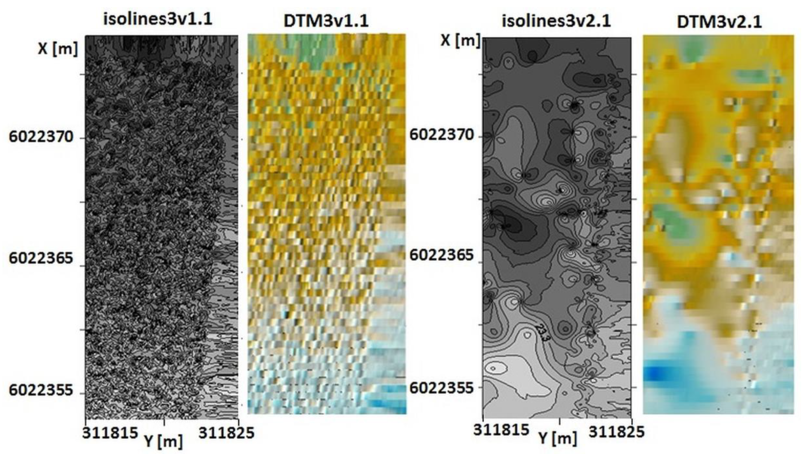
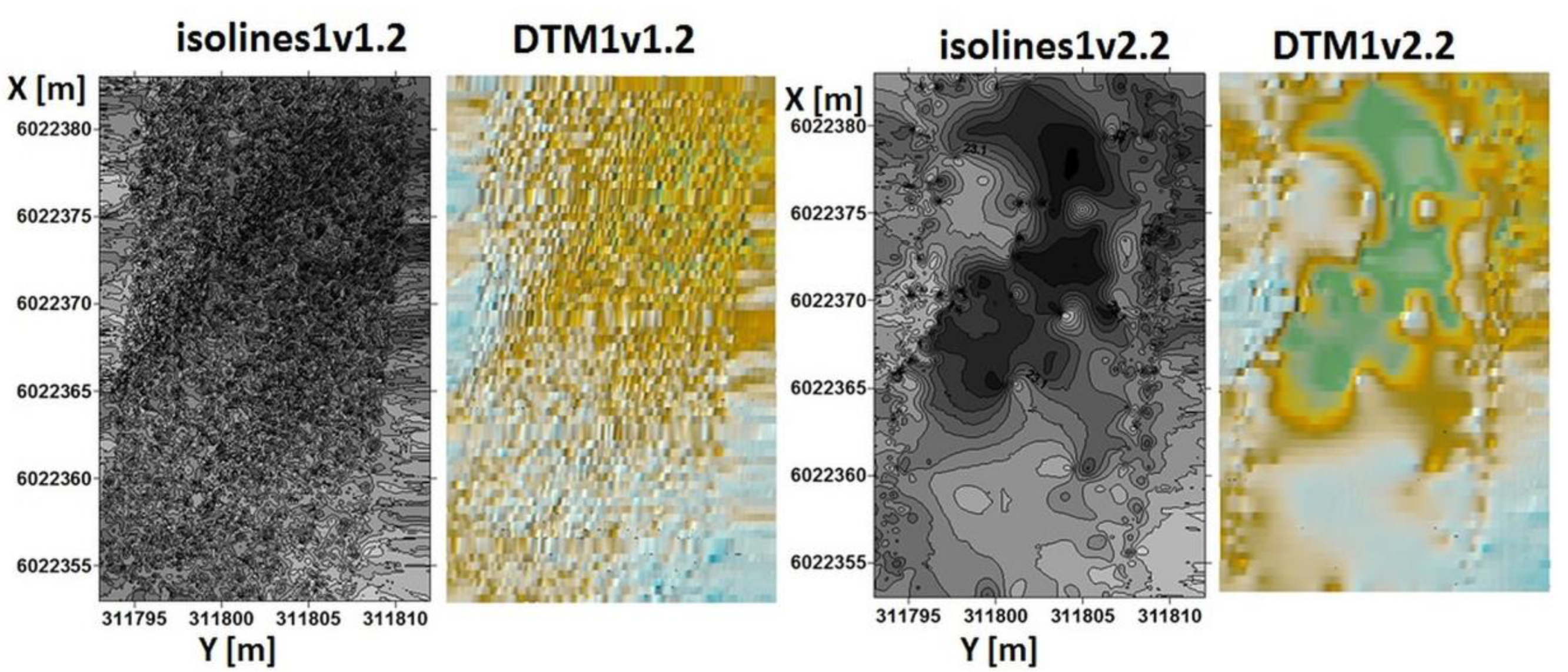
- The navigator has full control over the number of observations and the obtained DTMs are of good quality. In the case of isolines, mapping the obtained results shows that isolines generated by way of the OptD method are more readable and these isolines present more visible depths.
Author Contributions
Funding
Acknowledgments
Conflicts of Interest
References
- Chen, P.; Li, Y.; Su, Y.; Chen, X.; Jiang, Y. Review of AUV Underwater Terrain Matching Navigation. J. Navig. 2015, 68, 1155–1172. [Google Scholar] [CrossRef]
- Chen, P.-Y.; Li, Y.; Su, Y.-M.; Chen, X.-L.; Jiang, Y.-Q. Underwater terrain positioning method based on least squares estimation for AUV. China Ocean Eng. 2015, 29, 859–874. [Google Scholar] [CrossRef]
- Claus, B.; Bachmayer, R. Terrain-aided Navigation for an Underwater Glider. J. Field Robot. 2015, 32, 935–951. [Google Scholar] [CrossRef]
- Hagen, O.; Anonsen, K.; Saebo, T. Toward Autonomous Mapping with AUVs—Line-to-Line Terrain Navigation. In Proceedings of the Oceans 2015-MTS/IEEE Washington, Washington, DC, USA, 19–22 October 2015. [Google Scholar]
- Jung, J.; Li, J.; Choi, H.; Myung, H. Localization of AUVs using visual information of underwater structures and artificial landmarks. Intell. Serv. Robot. 2017, 10, 67–76. [Google Scholar] [CrossRef]
- Salavasidis, G.; Harris, C.; McPhail, S.; Phillips, A.B.; Rogers, E. Terrain Aided Navigation for Long Range AUV Operations at Arctic Latitudes. In Proceedings of the 2016 IEEE/OES Autonomous Underwater Vehicles (AUV), Tokyo, Japan, 6–9 November 2016; pp. 115–123. [Google Scholar]
- Li, Y.; Ma, T.; Wang, R.; Chen, P.; Zhang, Q. Terrain Correlation Correction Method for AUV Seabed Terrain Mapping. J. Navig. 2017, 70, 1062–1078. [Google Scholar] [CrossRef]
- Dong, M.; Chou, W.; Fang, B. Underwater Matching Correction Navigation Based on Geometric Features Using Sonar Point Cloud Data. Sci. Program. 2017, 2017, 7136702. [Google Scholar] [CrossRef]
- Song, Z.; Bian, H.; Zielinski, A. Application of acoustic image processing in underwater terrain aided navigation. Ocean Eng. 2016, 121, 279–290. [Google Scholar] [CrossRef]
- Ramesh, R.; Jyothi, V.B.N.; Vedachalam, N.; Ramadass, G.; Atmanand, M. Development and Performance Validation of a Navigation System for an Underwater Vehicle. J. Navig. 2016, 69, 1097–1113. [Google Scholar] [CrossRef]
- Li, Y.; Ma, T.; Chen, P.; Jiang, Y.; Wang, R.; Zhang, Q. Autonomous underwater vehicle optimal path planning method for seabed terrain matching navigation. Ocean Eng. 2017, 133, 107–115. [Google Scholar] [CrossRef]
- Li, Y.; Ma, T.; Wang, R.; Chen, P.; Shen, P.; Jiang, Y. Terrain Matching Positioning Method Based on Node Multi-information Fusion. J. Navig. 2017, 70, 82–100. [Google Scholar] [CrossRef]
- Stuntz, A.; Kelly, J.S.; Smith, R.N. Enabling Persistent Autonomy for Underwater Gliders with Ocean Model Predictions and Terrain-Based Navigation. Front. Robot. AI 2016, 3, 23. [Google Scholar] [CrossRef]
- Wang, L.; Yu, L.; Zhu, Y. Construction Method of the Topographical Features Model for Underwater Terrain Navigation. Pol. Marit. Res. 2015, 22, 121–125. [Google Scholar] [CrossRef][Green Version]
- Wei, F.; Yuan, Z.; Zhe, R. UKF-Based Underwater Terrain Matching Algorithms Combination. In Proceedings of the 2015 International Industrial Informatics and Computer Engineering Conference, Xi’an, China, 10–11 January 2015; pp. 1027–1030. [Google Scholar]
- Zhou, L.; Cheng, X.; Zhu, Y. Terrain aided navigation for autonomous underwater vehicles with coarse maps. Meas. Sci. Technol. 2016, 27, 095002. [Google Scholar] [CrossRef]
- Zhou, L.; Cheng, X.; Zhu, Y.; Dai, C.; Fu, J. An Effective Terrain Aided Navigation for Low-Cost Autonomous Underwater Vehicles. Sensors 2017, 17, 680. [Google Scholar] [CrossRef] [PubMed]
- Zhou, L.; Cheng, X.; Zhu, Y.; Lu, Y. Terrain Aided Navigation for Long-Range AUVs Using a New Bathymetric Contour Matching Method. In Proceedings of the 2015 IEEE International Conference on Advanced Intelligent Mechatronics (AIM), Busan, Korea, 7–11 July 2015. [Google Scholar]
- Calder, B.R.; Mayer, L.A. Automatic processing of high-rate, high-density multibeam echosounder data. Geochem. Geophys. Geosyst. 2003, 4, 1048. [Google Scholar] [CrossRef]
- Kulawiak, M.; Lubniewski, Z. Processing of LiDAR and multibeam sonar point cloud data for 3D surface and object shape reconstruction. In Proceedings of the 2016 Baltic Geodetic Congress (BGC Geomatics), Gdańsk, Poland, 2–4 June 2016. [Google Scholar] [CrossRef]
- Maleika, W. Moving Average Optimization in Digital Terrain Model Generation Based on Test Multibeam Echosounder Data. Geo Mar. Lett. 2015, 35, 61–68. [Google Scholar] [CrossRef]
- Maleika, W. The Influence of the Grid Resolution on the Accuracy of the Digital Terrain Model Used in Seabed Modelling. Mar. Geophys. Res. 2015, 36, 35–44. [Google Scholar] [CrossRef]
- Wlodarczyk-Sielicka, M. Interpolating Bathymetric Big Data for an Inland Mobile Navigation System. Inf. Technol. Control. 2018, 47, 338–348. [Google Scholar] [CrossRef]
- Wlodarczyk-Sielicka, M.; Wawrzyniak, N. Problem of Bathymetric Big Data Interpolation for Inland Mobile Navigation System. In Communications in Computer and Information Science, Proceedings of the 23rd International Conference on Information and Software Technologies (ICIST 2017), Druskininkai, Lithuania, 12–14 October 2017; Springer: Cham, Switzerland, 2017; Volume 756, pp. 611–621. [Google Scholar] [CrossRef]
- Wlodarczyk-Sielicka, M.; Lubczonek, J. The Use of an Artificial Neural Network to Process Hydrographic Big Data during Surface Modeling. Computer 2019, 8, 26. [Google Scholar] [CrossRef]
- Rezvani, M.-H.; Sabbagh, A.; Ardalan, A.A. Robust Automatic Reduction of Multibeam Bathymetric Data Based on M-estimators. Mar. Geod. 2015, 38, 327–344. [Google Scholar] [CrossRef]
- Yang, F.; Li, J.; Han, L.; Liu, Z. The filtering and compressing of outer beams to multibeam bathymetric data. Mar. Geophys. Res. 2013, 34, 17–24. [Google Scholar] [CrossRef]
- Zhang, T.; Xu, X.; Xu, S. Method of establishing an underwater digital elevation terrain based on kriging interpolation. Measurement 2015, 63, 287–298. [Google Scholar] [CrossRef]
- Wlodarczyk-Sielicka, M. Importance of Neighborhood Parameters During Clustering of Bathymetric Data Using Neural Network. In Communications in Computer and Information Science, Proceedings of the 22nd International Conference on Information and Software Technologies (ICIST 2016), Druskininkai, Lithuania, 13–15 October 2016; Springer: Cham, Switzerland, 2016; Volume 639, pp. 441–452. [Google Scholar] [CrossRef]
- Lubczonek, J.; Borawski, M. A New Approach to Geodata Storage and Processing Based on Neural Model of the Bathymetric Surface. In Proceedings of the 2016 Baltic Geodetic Congress (BGC Geomatics), Gdansk, Poland, 2–4 June 2016; pp. 1–7. [Google Scholar] [CrossRef]
- Specht, C.; Świtalski, E.; Specht, M. Application of an Autonomous/Unmanned Survey Vessel (ASV/USV) in Bathymetric Measurements. Pol. Marit. Res. 2017, 24, 36–44. [Google Scholar] [CrossRef]
- Moszynski, M.; Chybicki, A.; Kulawiak, M.; Lubniewski, Z. A novel method for archiving multibeam sonar data with emphasis on efficient record size reduction and storage. Pol. Marit. Res. 2013, 20, 77–86. [Google Scholar] [CrossRef]
- Kogut, T.; Niemeyer, J.; Bujakiewicz, A. Neural networks for the generation of sea bed models using airborne lidar bathymetry data. Geod. Cartogr. 2016, 65, 41–54. [Google Scholar] [CrossRef]
- Aykut, N.O.; Akpınar, B.; Aydın, Ö. Hydrographic data modeling methods for determining precise seafloor topography. Comput. Geosci. 2013, 17, 661–669. [Google Scholar] [CrossRef]
- Blaszczak-Bak, W. New Optimum Dataset method in LiDAR processing. Acta Geodyn. Geomater. 2016, 13, 379–386. [Google Scholar] [CrossRef]
- Błaszczak-Bąk, W.; Koppanyi, Z.; Toth, C. Reduction Method for Mobile Laser Scanning Data. ISPRS Int. J. Geo Inf. 2018, 7, 285. [Google Scholar] [CrossRef]
- Błaszczak-Bąk, W.; Sobieraj-Żłobińska, A.; Kowalik, M. The OptD-multi method in LiDAR processing. Meas. Sci. Technol. 2017, 28, 75009. [Google Scholar] [CrossRef]
- Kazimierski, W.; Wlodarczyk-Sielicka, M. Technology of Spatial Data Geometrical Simplification in Maritime Mobile Information System for Coastal Waters. Pol. Marit. Res. 2016, 23, 3–12. [Google Scholar] [CrossRef][Green Version]
- Stateczny, A.; Gronska-Sledz, D.; Motyl, W. Precise Bathymetry as a Step Towards Producing Bathymetric Electronic Navigational Charts for Comparative (Terrain Reference) Navigation. J. Navig. 2019. [Google Scholar] [CrossRef]
- Borkowski, P.; Pietrzykowski, Z.; Magaj, J.; Mąka, M. Fusion of data from GPS receivers based on a multi-sensor Kalman filter. Transp. Probl. 2008, 3, 5–11. [Google Scholar]
- Donovan, G.T. Position Error Correction for an Autonomous Underwater Vehicle Inertial Navigation System (INS) Using a Particle Filter. IEEE J. Ocean. Eng. 2012, 37, 431–445. [Google Scholar] [CrossRef]
- Wawrzyniak, N.; Stateczny, A. MSIS Image Positioning in Port Areas with the Aid of Comparative Navigation Methods. Pol. Marit. Res. 2017, 24, 32–41. [Google Scholar] [CrossRef]
- Ping DSP, Products Description. Available online: http://www.pingdsp.com/3DSS-DX-450 (accessed on 9 May 2019).
- Stateczny, A.; Wlodarczyk-Sielicka, M.; Gronska, D.; Motyl, W. Multibeam Echosounder and Lidar in Process of 360° Numerical Map Production for Restricted Waters with Hydrodron. In Proceedings of the 2018 Baltic Geodetic Congress (BGC Geomatics) Gdansk, Olsztyn, Poland, 21–23 June 2018. [Google Scholar] [CrossRef]
- Douglas, D.; Peucker, T. Algorithms for the reduction of the number of points required to represent a digitized line or its caricature. Cartographica 1973, 10, 112–122. [Google Scholar] [CrossRef]
- Fei, L.; Jin, H. A three-dimensional Douglas–Peucker algorithm and its application to automated generalization of DEMs. Int. J. Geogr. Inf. Sci. 2009, 23, 703–718. [Google Scholar] [CrossRef]
- Zeng, X.; He, W. GPGPU Based Parallel processing of Massive LiDAR Point Cloud. In Proceedings of the MIPPR 2009: Medical Imaging, Parallel Processing of Images, and Optimization Techniques. International Society for Optics and Photonics, Yichang, China, 30 October–1 November 2009; Volume 7497. [Google Scholar]
- Chen, Y. High Performance Computing for Massive LiDAR Data Processing with Optimized GPU Parallel Programming. Master’s Thesis, The University of Texas at Dallas, Richardson, TX, USA, 2012. [Google Scholar]
- Cao, J.; Cui, H.; Shi, H.; Jiao, L. Big Data: A Parallel Particle Swarm Optimization-Back-Propagation Neural Network Algorithm Based on MapReduce. PLoS ONE 2016, 11, e0157551. [Google Scholar] [CrossRef] [PubMed]
- Liu, S.; Wang, L.; Liu, H.; Su, H.; Li, X.; Zheng, W. Deriving Bathymetry from Optical Images with a Localized Neural Network Algorithm. IEEE Trans. Geosci. Remote Sens. 2018, 56, 5334–5342. [Google Scholar] [CrossRef]
- Lubczonek, J. Hybrid neural model of the sea bottom surface. In Lecture Notes in Computer Science, Proceedings of the International Conference on Artificial Intelligence and Soft Computing (ICAISC), Zakopane, Poland, 7–11 June 2004; Springer: Berlin/Heidelberg, Germany, 2004; Volume 3070, pp. 1154–1160. [Google Scholar]


| Number of Points | H min. [m] | H max. [m] | R [m] | STD [m] | ||
|---|---|---|---|---|---|---|
| Whole dataset | 694185 | 15.08 | 23.65 | 8.57 | 2.44 | |
| Strips without overlay | p1 | 54176 | 22.86 | 23.54 | 0.68 | 0.08 |
| p2 | 35106 | 22.86 | 23.60 | 0.74 | 0.11 | |
| p3 | 44333 | 22.82 | 23.58 | 0.76 | 0.12 | |
| p4 | 53579 | 22.75 | 23.65 | 0.90 | 0.10 | |
| p5 | 52967 | 22.64 | 23.52 | 0.88 | 0.11 | |
| p6 | 55497 | 22.04 | 23.39 | 1.35 | 0.20 | |
| p7 | 70704 | 20.84 | 23.14 | 2.30 | 0.40 | |
| p8 | 84962 | 19.48 | 22.16 | 2.68 | 0.55 | |
| p9 | 79890 | 17.86 | 20.42 | 2.56 | 0.49 | |
| p10 | 53216 | 17.35 | 18.78 | 1.43 | 0.27 | |
| p11 | 55373 | 16.36 | 18.04 | 1.68 | 0.33 | |
| p12 | 54382 | 15.08 | 17.03 | 1.95 | 0.31 | |
| Strips with overlay | po1 | 72718 | 22.86 | 23.54 | 0.68 | 0.09 |
| po2 | 56075 | 22.82 | 23.60 | 0.78 | 0.12 | |
| po3 | 72478 | 22.75 | 23.65 | 0.90 | 0.11 | |
| po4 | 80936 | 22.73 | 23.65 | 0.92 | 0.10 | |
| po5 | 80642 | 22.40 | 23.52 | 1.12 | 0.14 | |
| po6 | 90022 | 21.50 | 23.39 | 1.89 | 0.29 | |
| po7 | 115584 | 20.18 | 23.16 | 2.98 | 0.62 | |
| po8 | 122894 | 18.75 | 22.21 | 3.46 | 0.75 | |
| po9 | 101810 | 17.71 | 20.42 | 2.71 | 0.56 | |
| po10 | 84810 | 16.92 | 18.78 | 1.86 | 0.41 | |
| po11 | 84551 | 15.82 | 18.04 | 2.22 | 0.44 | |
| po12 | 54592 | 15.08 | 17.04 | 1.96 | 0.31 |
| Number of Points | H min. [m] | H max. [m] | R [m] | STD [m] | ||
|---|---|---|---|---|---|---|
| Optimized dataset | 13976 | 15.10 | 23.57 | 8.47 | 2.86 | |
| Strips without overlay | p1 | 1091 | 22.86 | 23.53 | 0.67 | 0.11 |
| p2 | 702 | 22.86 | 23.57 | 0.71 | 0.13 | |
| p3 | 888 | 22.85 | 23.57 | 0.72 | 0.13 | |
| p4 | 1071 | 22.75 | 23.65 | 0.90 | 0.13 | |
| p5 | 1055 | 22.72 | 23.52 | 0.80 | 0.14 | |
| p6 | 1111 | 22.05 | 23.35 | 1.30 | 0.25 | |
| p7 | 1403 | 20.84 | 23.10 | 2.26 | 0.55 | |
| p8 | 1710 | 19.50 | 22.16 | 2.66 | 0.78 | |
| p9 | 1605 | 17.86 | 20.38 | 2.52 | 0.71 | |
| p10 | 1066 | 17.40 | 18.76 | 1.36 | 0.36 | |
| p11 | 1116 | 16.36 | 18.00 | 1.64 | 0.50 | |
| p12 | 1079 | 15.10 | 17.01 | 1.91 | 0.46 | |
| Strips with overlay | po1 | 1446 | 22.86 | 23.54 | 0.68 | 0.13 |
| po2 | 1132 | 22.86 | 23.60 | 0.74 | 0.13 | |
| po3 | 1444 | 22.81 | 23.65 | 0.84 | 0.14 | |
| po4 | 1633 | 22.77 | 23.65 | 0.88 | 0.14 | |
| po5 | 1619 | 22.42 | 23.52 | 1.10 | 0.21 | |
| po6 | 1794 | 21.56 | 23.38 | 1.82 | 0.42 | |
| po7 | 2321 | 20.26 | 23.11 | 2.85 | 0.86 | |
| po8 | 2456 | 18.76 | 22.19 | 3.43 | 1.08 | |
| po9 | 2018 | 17.71 | 20.42 | 2.71 | 0.80 | |
| po10 | 1691 | 16.92 | 18.77 | 1.85 | 0.62 | |
| po11 | 1689 | 15.91 | 18.01 | 2.10 | 0.65 | |
| po12 | 1094 | 15.10 | 16.96 | 1.86 | 0.46 |
| DTM | H min. [m] | H max. [m] | STD [m] | Time [s] for Generated DTMs |
|---|---|---|---|---|
| DTM1v1.1 DTM1v2.1 | 22.88 22.85 | 23.48 23.47 | 0.08 0.09 | 14 14 |
| DTM2v1.1 DTM2v2.1 | 22.87 22.87 | 23.57 23.53 | 0.12 0.12 | 12 10 |
| DTM3v1.1 DTM3v2.1 | 22.83 22.83 | 23.54 23.54 | 0.13 0.14 | 11 9 |
| DTM4v1.1 DTM4v2.1 | 22.80 22.79 | 23.54 23.60 | 0.13 0.12 | 15 12 |
| DTM5v1.1 DTM5v2.1 | 22.67 22.65 | 23.51 23.51 | 0.12 0.13 | 13 11 |
| DTM6v1.1 DTM6v2.1 | 22.70 22.67 | 23.38 23.33 | 0.22 0.24 | 14 10 |
| DTM7v1.1 DTM7v2.1 | 20.79 20.77 | 23.12 23.12 | 0.44 0.47 | 13 9 |
| DTM8v1.1 DTM8v2.1 | 19.43 19.45 | 22.09 22.09 | 0.58 0.59 | 14 10 |
| DTM9v1.1 DTM9v2.1 | 17.99 17.96 | 20.40 20.37 | 0.55 0.55 | 16 12 |
| DTM10v1.1 DTM10v2.1 | 17.35 17.37 | 18.76 18.74 | 0.31 0.32 | 12 10 |
| DTM11v1.1 DTM11v2.1 | 16.37 16.36 | 18.02 17.99 | 0.39 0.40 | 12 9 |
| DTM12v1.1 DTM12v2.1 | 15.16 15.15 | 17.01 17.01 | 0.29 0.29 | 13 10 |
| DTM | H min. [m] | H max. [m] | STD [m] | Time [s] for Generated DTMS |
|---|---|---|---|---|
| DTM1v1.2 DTM1v2.2 | 22.87 22.86 | 23.47 23.50 | 0.09 0.12 | 20 19 |
| DTM2v1.2 DTM2v2.2 | 22.86 22.87 | 23.52 23.53 | 0.12 0.13 | 21 18 |
| DTM3v1.2 DTM3v2.2 | 22.80 22.82 | 23.54 23.55 | 0.12 0.12 | 23 19 |
| DTM4v1.2 DTM4v2.2 | 22.82 22.79 | 23.54 23.55 | 0.11 0.13 | 22 18 |
| DTM5v1.2 DTM5v2.2 | 22.43 22.46 | 23.50 23.51 | 0.15 0.16 | 21 17 |
| DTM6v1.2 DTM6v2.2 | 21.52 21.53 | 23.41 23.39 | 0.31 0.32 | 21 16 |
| DTM7v1.2 DTM7v2.2 | 20.23 20.25 | 23.12 23.09 | 0.67 0.68 | 22 16 |
| DTM8v1.2 DTM8v2.2 | 18.76 18.76 | 22.15 22.16 | 0.81 0.82 | 22 15 |
| DTM9v1.2 DTM9v2.2 | 17.75 17.71 | 20.39 20.42 | 0.63 0.65 | 24 16 |
| DTM10v1.2 DTM10v2.2 | 16.95 16.96 | 18.76 18.75 | 0.43 0.45 | 19 14 |
| DTM11v1.2 DTM11v2.2 | 15.81 15.83 | 18.02 18.00 | 0.49 0.50 | 23 16 |
| DTM12v1.2 DTM12v2.2 | 15.16 15.17 | 17.02 16.99 | 0.29 0.28 | 22 16 |
| DTM | H min. [m] | H max. [m] | STD [m] | Time [s] for Generated DTMS |
|---|---|---|---|---|
| DTM100% DTM2% | 15.29 15.32 | 23.56 23.56 | 2.50 2.54 | 268 150 |
| ΔH min. [m] | ΔH max. [m] | ΔHmean [m] | STD [m] | ||
|---|---|---|---|---|---|
| Strips without overlay | p1–p2 | −0.32 | 0.32 | 0.01 | 0.08 |
| p2–p3 | −0.22 | 0.27 | 0.00 | 0.02 | |
| p3–p4 | −0.37 | 0.30 | −0.01 | 0.08 | |
| p4–p5 | −0.49 | 0.28 | −0.02 | 0.08 | |
| p5–p6 | −0.36 | 0.30 | −0.02 | 0.07 | |
| p6–p7 | −0.40 | 0.32 | −0.03 | 0.08 | |
| p7–p8 | −0.60 | 0.29 | −0.09 | 0.13 | |
| p8–p9 | −0.58 | 0.27 | −0.06 | 0.11 | |
| p9–p10 | −0.80 | 0.23 | −0.06 | 0.11 | |
| p10–p11 | −0.52 | 0.19 | −0.08 | 0.09 | |
| p11–p12 | −0.43 | 0.22 | −0.03 | 0.07 | |
| Strips with overlay | po1–po2 | −0.26 | 0.22 | 0.00 | 0.05 |
| po2–po3 | −0.33 | 0.33 | 0.00 | 0.05 | |
| po3–po4 | −0.31 | 0.25 | −0.01 | 0.04 | |
| po4–po5 | −0.26 | 0.24 | 0.00 | 0.04 | |
| po5–po6 | −0.28 | 0.24 | 0.00 | 0.04 | |
| po6–po7 | −0.37 | 0.28 | −0.03 | 0.07 | |
| po7–po8 | −0.56 | 0.21 | −0.04 | 0.10 | |
| po8–po9 | −0.43 | 0.20 | −0.03 | 0.07 | |
| po9–po10 | −0.52 | 0.24 | −0.03 | 0.07 | |
| po10–po11 | −0.38 | 0.25 | −0.02 | 0.05 | |
| po11–po12 | −0.43 | 0.42 | −0.01 | 0.06 |
| ΔH min. [m] | ΔH max. [m] | ΔHmean [m] | STD [m] | ||
|---|---|---|---|---|---|
| Strips without overlay | p1–p2 | −0.21 | 0.34 | 0.03 | 0.07 |
| p2–p3 | −0.29 | 0.28 | 0.00 | 0.11 | |
| p3–p4 | −0.22 | 0.25 | 0.00 | 0.07 | |
| p4–p5 | −0.34 | 0.21 | −0.02 | 0.07 | |
| p5–p6 | −0.31 | 0.23 | −0.02 | 0.09 | |
| p6–p7 | −0.24 | 0.24 | −0.03 | 0.07 | |
| p7–p8 | −0.44 | 0.26 | −0.08 | 0.11 | |
| p8–p9 | −0.55 | 0.28 | −0.10 | 0.13 | |
| p9–p10 | −0.49 | 0.27 | −0.04 | 0.08 | |
| p10–p11 | −0.40 | 0.18 | −0.06 | 0.08 | |
| p11–p12 | −0.44 | 0.17 | −0.04 | 0.07 | |
| Strips with overlay | po1–po2 | −0.21 | 0.27 | −0.01 | 0.08 |
| po2–po3 | −0.20 | 0.05 | −0.06 | 0.07 | |
| po3–po4 | −0.26 | 0.26 | 0.07 | 0.07 | |
| po4–po5 | −0.29 | 0.20 | −0.02 | 0.08 | |
| po5–po6 | −0.20 | 0.20 | 0.03 | 0.06 | |
| po6–po7 | −0.31 | 0.33 | −0.03 | 0.12 | |
| po7–po8 | −0.52 | 0.24 | −0.11 | 0.14 | |
| po8–po9 | −0.70 | 0.28 | −0.06 | 0.19 | |
| po9–po10 | −0.35 | 0.26 | 0.02 | 0.08 | |
| po10–po11 | −0.39 | 0.47 | 0.03 | 0.16 | |
| po11–po12 | −0.37 | 0.53 | 0.05 | 0.15 |
| Methodology v1 | |||||
|---|---|---|---|---|---|
| ΔH min. [m] | ΔH max. [m] | ΔHmean [m] | STD [m] | ||
| Strips without overlay | Min. | −0.80 | 0.19 | −0.09 | 0.02 |
| Max. | −0.22 | 0.32 | 0.01 | 0.13 | |
| Mean | −0.46 | 0.29 | −0.03 | 0.08 | |
| Standard deviation | 0.16 | 0.04 | 0.03 | 0.03 | |
| Strips with overlay | Min. | −0.56 | 0.20 | −0.04 | 0.04 |
| Max. | −0.26 | 0.42 | 0.00 | 0.10 | |
| Mean | −0.38 | 0.26 | −0.01 | 0.06 | |
| Standard deviation | 0.10 | 0.06 | 0.01 | 0.02 | |
| Methodology v2 | |||||
|---|---|---|---|---|---|
| ΔH min. [m] | ΔH max. [m] | ΔHmean [m] | STD [m] | ||
| Strips without overlay | Min. | −0.55 | 0.17 | −0.10 | 0.07 |
| Max. | −0.21 | 0.34 | 0.03 | 0.13 | |
| Mean | −0.34 | 0.26 | −0.03 | 0.09 | |
| Standard deviation | 0.12 | 0.05 | 0.04 | 0.02 | |
| Strips with overlay | Min. | −0.70 | 0.05 | −0.11 | 0.06 |
| Max. | −0.20 | 0.53 | 0.07 | 0.19 | |
| Mean | −0.35 | 0.28 | −0.01 | 0.11 | |
| Standard deviation | 0.15 | 0.13 | 0.05 | 0.04 | |
| Methodology v1—Methodology v2 | |||||
|---|---|---|---|---|---|
| ΔH min. [m] | ΔH max. [m] | ΔHmean [m] | STD [m] | ||
| Strips without overlay | Min. | −0.25 | 0.02 | 0.01 | −0.05 |
| Max. | −0.01 | −0.02 | −0.02 | 0.01 | |
| Mean | −0.12 | 0.02 | 0.00 | 0.00 | |
| Standard deviation | 0.04 | −0.01 | 0.00 | 0.01 | |
| Strips with overlay | Min. | 0.14 | 0.15 | 0.07 | −0.03 |
| Max. | −0.05 | −0.11 | −0.07 | −0.09 | |
| Mean | −0.03 | −0.02 | −0.01 | −0.05 | |
| Standard deviation | −0.05 | −0.07 | −0.04 | −0.03 | |
| Strips with Overlay—Strips without Overlay | ||||
|---|---|---|---|---|
| ΔH min. [m] | ΔH max. [m] | ΔHmean [m] | STD [m] | |
| Min. | −0.15 | −0.12 | −0.01 | 0.00 |
| Max. | 0.01 | 0.19 | 0.05 | 0.06 |
| Mean | 0.00 | 0.02 | 0.02 | 0.02 |
| Standard deviation | 0.04 | 0.08 | 0.02 | 0.02 |
© 2019 by the authors. Licensee MDPI, Basel, Switzerland. This article is an open access article distributed under the terms and conditions of the Creative Commons Attribution (CC BY) license (http://creativecommons.org/licenses/by/4.0/).
Share and Cite
Stateczny, A.; Błaszczak-Bąk, W.; Sobieraj-Żłobińska, A.; Motyl, W.; Wisniewska, M. Methodology for Processing of 3D Multibeam Sonar Big Data for Comparative Navigation. Remote Sens. 2019, 11, 2245. https://doi.org/10.3390/rs11192245
Stateczny A, Błaszczak-Bąk W, Sobieraj-Żłobińska A, Motyl W, Wisniewska M. Methodology for Processing of 3D Multibeam Sonar Big Data for Comparative Navigation. Remote Sensing. 2019; 11(19):2245. https://doi.org/10.3390/rs11192245
Chicago/Turabian StyleStateczny, Andrzej, Wioleta Błaszczak-Bąk, Anna Sobieraj-Żłobińska, Weronika Motyl, and Marta Wisniewska. 2019. "Methodology for Processing of 3D Multibeam Sonar Big Data for Comparative Navigation" Remote Sensing 11, no. 19: 2245. https://doi.org/10.3390/rs11192245
APA StyleStateczny, A., Błaszczak-Bąk, W., Sobieraj-Żłobińska, A., Motyl, W., & Wisniewska, M. (2019). Methodology for Processing of 3D Multibeam Sonar Big Data for Comparative Navigation. Remote Sensing, 11(19), 2245. https://doi.org/10.3390/rs11192245