Article

Satellite Monitoring of Thermal Performance in Smart Urban Designs

by
Daniela Mullerova
1 and
Meredith Williams
2,*
1
Independent Researcher, Rochester, Kent, UK
2
School of Science, Medway Campus, University of Greenwich, Central Avenue, Chatham Maritime, Kent ME4 4TB, UK
*
Author to whom correspondence should be addressed.
Remote Sens. 2019, 11(19), 2244; https://doi.org/10.3390/rs11192244
Submission received: 1 August 2019 / Revised: 3 September 2019 / Accepted: 15 September 2019 / Published: 26 September 2019
(This article belongs to the Section Urban Remote Sensing)

Abstract

:
Climate change amplified by rapidly increasing urbanization is resulting in rising temperatures within urban environments. In recent years, to mitigate this the design and construction of new buildings has emphasized “smart” methods and materials for individual buildings rather than landscape-level planning and evaluation of new developments. Remote Sensing potentially offers a cost-effective means to monitor effectiveness of landscape-level urban design and guide developers to improve thermal regimes. This paper focuses on satellite monitoring of thermal variation in the area of London most affected by construction in 2010–2015. Split-window Land Surface Temperature (LST) models were applied to ASTER and Landsat 8 satellite imagery, requiring separate investigation of thermal trends due to temporal inconsistency. Getis-Ord-Gi* cluster analysis of the ASTER image identified three main thermal hot spots: Eastern, Stratford railway/underground station, and Stratford High Street. It is assumed that increased thermal stress within these areas is mainly from anthropogenic heat. However, local thermal variations for Eastern Olympic Village are attributed to changing meteorological conditions, facade materials, canyon morphology and orientation, or insufficient shading and ventilation. Future development of a new cultural hub at this location will significantly affect distribution of green spaces and influence their cooling ability.

Graphical Abstract

1. Introduction

An Urban Heat Island (UHI) occurs where temperature in an urban area exceeds that of the surrounding rural area. UHIs are dependent on spatial arrangements and interactions between urban and rural areas within the landscape, as the rate of cooling in urban areas is much slower in comparison to the rural areas [1]. Thermal imbalance between rural and urban environments is increasing with the modification of urban climates. Although there are many influencing factors in play, increasing urban density caused by continual growth of urban population, affected by the lack of urban space, and land cover change from vegetated to built-up materials, are considered two of the main driving factors [2]. Modification of urban climates is further amplified by the current effects of climate change [1,3], which consequently influences the increase in demand for electricity, used for cooling or heating [4] (Figure 1).
UHIs as defined by [5] and [6] are distinctive layers of the urban atmosphere related not only to the different surfaces but also sub-surfaces and can be established for Urban Boundary Layer (UBL) and Urban Canopy Layer (UCL). However, the first application of remote sensing methods to UHIs conducted by [7] required the identification of a Surface Urban Heat Island (SUHI), later described by [3] as a thermal radiance detected by remote sensing corrected for atmosphere transmissivity and surface emissivity. Atmospheric corrections can be performed by a number of methods that use different atmospheric models. The variables that play a vital role in thermodynamic processes ongoing in the lower layer of the atmosphere, close to the urban surfaces, are complex and turbulent; therefore, their combined effects must be taken into account [3].
Urban Heat Island Intensity (UHII), comprising Atmospheric (AUHII) and Surface (SUHII), is a very important element in current urban planning, hence assessment of their effects is absolutely essential [8]. AUHII is mostly retrieved from weather stations and SUHII from satellite remote sensing [2]. For a summary review of UHI analysis from satellite imagery the reader is referred to [8]. The effects of UHIs can be observed almost exclusively where natural surfaces have been altered by humans and their intensity can be influenced by factors such as (1) decreased albedo, smaller amount of vegetation or higher roughness of surfaces [9,10], (2) increase in the temperature caused by humans such as density of traffic in the city, density or structure of buildings, and human metabolism [11]. There is a direct causality between the recorded increase in temperature and increasing amount of energy emitted by the sun soon after the sunrise. Moisture in the ground and in the bodies of plants reduces the rate of increase in rural areas [12] compared to the urban areas. Soon after sunset the cooling rate is much higher in rural than urban environments [10], due to its dependency upon the reduction of radiative emissivity, caused by inherent properties of the urban surfaces. However, UHI can be also affected by other factors, such as land cover/land use [13], form of urban spaces—‘urban canyons’ [14,15]—or by the heterogeneity of building materials. Turbulent conditions within the urban sub-layers are regarded as a driving factor in development of UHIs, not only at the rural to urban scale but also at more complex local scales, dependent upon the particular morphology and urban heterogeneity.
Smart or sustainable materials, including the new ways of building management are emphasized in current urban developments and widely studied. Better insulation, shading of open spaces, facade reflectance reduction, and implementation of green spaces within urban areas are typical of the solutions currently in use [16]. However, research has traditionally focused on the need to understand and improve the poor thermal properties of old buildings within urban environments. Landscape-level thermal properties of urban areas built according to the new standards have not been widely studied by remote sensing methods. Changing trends present the need to understand and monitor the performance of modern smart designs, with the potential to influence the distribution of thermal energy and consequently improve the living conditions within modern urban spaces.
The population of Greater London is expected to increase from 2011 to 2021 by one million [17], and by 2036 it is predicted there will be over 10 million inhabitants [18]. Problems related to the expected level of urbanization are becoming more pressing than ever. Based on the trends prior to 2013, the “Smart London Plan” [17] has been adopted, followed by its update “Future of Smart” [18]. Both plans were formulated with sustainable interests in mind, not only with regard to the environment and reduction of greenhouse gases, but also management of utilities and energy supplies. Thermal strains in the city, amplified by climate change, are expected to become more significant in the near future. Following the economical improvements that affected the construction industry after 2003 [19], with the additional prospects of London hosting the Olympic Games in 2012, some parts of London experienced a higher level of construction activity during the years 2010 to 2015, and this trend continues up to the present day. The urban developments built during this period used mostly new materials aimed at making individual buildings smarter and more efficient in terms of emissivity and the distribution and transmission of thermal energy. The goal of this study is to demonstrate whether freely available satellite thermal imagery has the potential to cost-effectively identify areas of new urban development in London where thermal performance at a landscape level is poor despite the incorporation of smart design and materials at individual building level. Such information has the potential to inform planning decisions in the many areas of London that are currently undergoing redevelopment or regeneration.

2. Study Area, Materials, and Methods

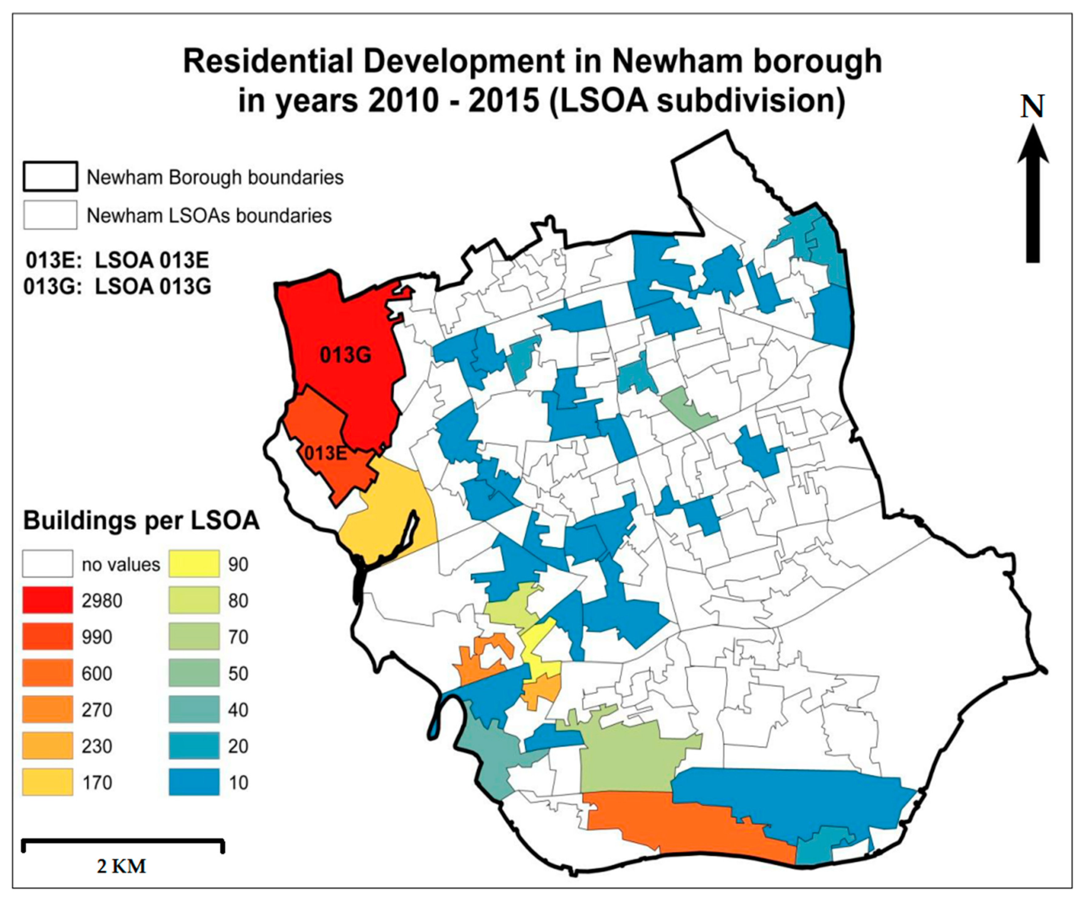
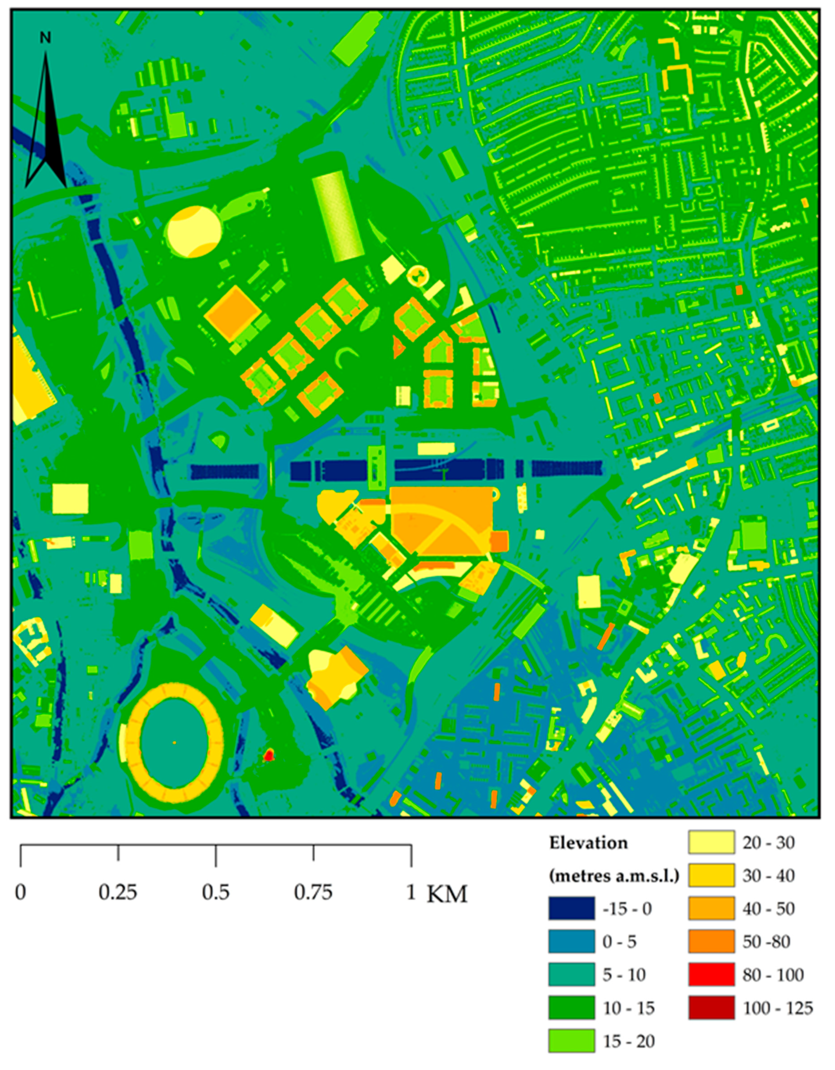
2.1. Choice of Study Area

The UHI phenomenon was first identified in London in 1833 [20]. A wide variety of approaches to characterizing Urban Heat Island effects in London have been carried out in recent years, at a range of spatial scales [20,21,22,23]. A variety of remote sensing techniques and data sources have been employed to study UHI effect in London, often hampered by cloudy weather conditions [20,21,22]. Additionally, several studies have involved direct measurement [24]. In [25] the authors examined the seasonal variations in the Surface Urban Heat Islands of London, based on the observations of the Urban Boundary Layer from MODIS satellite imagery and incorporation of the UrbClim model during heat incidents between the years 2006–2012. As the rate of heating of urban surfaces during the day is dependent on the solar irradiation, but the cooling rate of those surfaces overnight is more or less constant, seasonal differences in urban and rural areas should significantly affect the thermal balance. However, in the rural areas the heating up and cooling down is more influenced by the moisture present in the soil and the surrounding vegetation. Consequently, thermal variations between the urban and rural areas are expected to be the most profound during the period of June–July. This variation, however, proved to be less significant in the case of London than expected, which might be due to the unsynchronized meteorological and astronomical seasonality that affects background thermal properties and thermal properties in the city differently. A study of the influence of a range of variables on UHI in London was carried out by [21], who concluded that the most significant thermal changes within both day and night times were attributable to the surface albedo. Trend analysis was used, which proved that due to the cloudy nature of the climate over London the UHI values during the daytime were significantly higher on urban surfaces during partially cloudy conditions. However, the temperature was greatly affected by the presence of humans; therefore, the increase in the temperature was significantly higher in densely urbanized areas of London. A follow-on study by [22] presented the results of UHI intensity in London during the winter. This study recognized the necessity to understand the UHI characteristics during the winter period, which is essential in the building design processes as it can affect the energy performance of buildings and therefore influence the energy demands during winter. More recently, UHI studies of London have focused on addressing the problems related to energy performance of individual buildings and the dependency upon urban microclimates that can have a significant influence on sustainable urban designs [24]. Microclimatic conditions within the London metropolis are highly variable, and studies such as [24], conducted in the Southwark area, have shown that climatic factors are significantly influenced by urban texture. In [24] the authors concluded that the thermal/energy performance assessment of buildings need to be conducted using local microclimatic information, rather than the meteorological weather data mostly collected from non-urban environments. However, detailed study of these using field-based measurements is impractical over large areas, which is why this study has chosen to evaluate the suitability of satellite remote sensing to identify new build areas with UHI problems that require further finer spatial scale investigation. Quantitative Geographic Information System (GIS) analysis, detailed later in this section, identified the areas of Newham borough, Greater London, as the most affected by residential construction development in the period 2010–2015 (Figure 2). Calibrated Land Surface Temperature models were generated using satellite imagery from summer 2015, which determined the spatial thermal variations. Thermal patterns were compared to the expected patterns based upon previous scientific research, and problematic locations within areas of smart urban design identified. The results of spatial thermal analyses were independently validated by the project industrial partner—ARUP Engineering Consultancy, London.
The Dwelling age group counts data for London, based upon Lower Super Output Area (LSOA) hierarchy, were included in the quantitative analysis, performed for the period 2010–2015. The two LSOAs that contained the greatest number of new residential buildings were identified, with the codes 013G and 013E, containing respectively 2980 and 990 new residential buildings (Figure 3 and Figure 4). 013G and 013E are 1.586 and 0.566 sq. km respectively, giving an increase in residential building density of 1879 and 1749 new buildings per sq. km during the 2010–2015 study period. 013G and 013E are neighboring LSOAs that also belonged to the same borough, Newham, one of the most densely populated London boroughs. The 2010 Mid Year Estimate (MYE) population for Newham Borough was 299,171, rising to 332,800 in the 2015 MYE and 352,005 in the 2018 MYE, according to the Office for National Statistics. With an overall area of 38.58 sq. km that gives a population density for Newham of 7755 people per sq. km in 2010, increasing to 8627 per sq. km in 2015, an average annual increase of just over 2.2% per annum over the 5-year period covered by this study.
Much of the construction and urban development in Newham was related to the 2012 Olympic Games. Prior to the Games Newham borough received major financial investments from both the UK government and from private sources for redevelopment of targeted sites within the borough. This redevelopment is still ongoing within the location of Queen Elizabeth Olympic Park (Figure 5), with the potential loss of a significant amount of green space (see Figure 6d for vegetation fraction in 2015).
In a wider context, Stratford (Newham), offered the most homogenous study area (Figure 5), as the target was to find areas with a confirmed history of smart broad-scale development, built within the 2010–2015 time period, where buildings share similarities in regard to their shape and height. The LSOA dataset used already accounts for variations in population density, as the local LSOAs range in size between 1000 and 3000 inhabitants and 400 to 1200 households [26], therefore it was not considered necessary to normalize the values for population density. Including further normalization methods in the GIS analysis would affect the results significantly by highlighting more heterogeneous areas within the more densely populated central London.

2.2. Datasets Used for Land Surface Temperature Retrieval

Choosing the most suitable satellite imagery for this study proved to be a challenge. Landsat 7 Enhanced Thematic Mapper Plus (ETM+) was rejected, due to the large SLC-off data gaps [27]. A decision was made to use night-time thermal imagery from the Advanced Spaceborne Thermal Emission and Reflection Radiometer (ASTER) [28] with a spatial resolution of 90 m, and day-time thermal imagery from Landsat 8 TIRS with a spatial resolution of 100 m (resampled to 30 m) [29], due to the limited availability of cloud-free imagery within the study area. It has been proven that temperature differences between vegetated and man-made structures are more profound after sunset [12,30]. Additionally, according to [25], the intensity of UHI in the UK is typically highest around the 21 June (summer solstice) and background temperature is typically highest approximately on the border of July and August. Given these constraints the most suitable night-time thermal image identified was ASTER L1T level scene 59/220, from an ascending Terra overpass with an acquisition time of 9:45:25 p.m. U.T. on 6 August 2015. This ASTER scene did not contain Short Wave Infrared (SWIR) or visible bands, so for that reason the closest date Landsat 8 Operational Land Imager and Thermal Infra-Red Scanner (OLI/TIRS) imagery with minimal cloud cover was obtained. This was a day-time Landsat 8 OLI/TIRS L1T corrected scene 202/24 with acquisition time of 10:58:01 a.m. U.T. on 15 August 2015. This Landsat 8 scene was used both for incorporation into the emissivity estimate for the ASTER scene and for calculation of a Landsat-derived daytime LST image. The 9-day time gap was considered sufficiently small to assume no major changes in land cover occurred between the two image dates.

2.3. Land Surface Temperature Calculation

Calculation of brightness temperature required the conversion from raw digital numbers (DN) to spectral radiance, based on inclusion of maximum radiances for ASTER bands published by [31] and Unit Conversion Coefficients (UCC) published by [32]. In [32] the authors also provided the Calibration Constants needed during the conversion from spectral radiance to Top of Atmosphere (TOA) brightness temperature for the ASTER imagery. The standardized pre-processing procedures of [32] for ASTER, and [33] for Landsat 8 were used to derive spectral radiance. Established pre-processing methods and calibration coefficients were chosen, based on the available satellite imagery, and standardized approaches developed by [32,33] were adopted for ASTER and OLI/TIRS respectively. Unfortunately, the approach developed by [33] does not include a conversion from air temperature to surface temperature, therefore it was necessary to apply an additional stage to convert to Land Surface Temperature (LST). For the retrieval of LST the estimation of emissivity is very important, as the surface of the Earth is not a Blackbody, so emissivity must be included in the calculation of thermal radiance. Estimates can be based on field validation, atmospheric models, or vegetation indices such as the Normalized Difference Vegetation Index (NDVI). A range of approaches is available depending on the sensor type and the availability of atmospheric data. A study conducted by [34] compared various models and algorithms used for the processing of ASTER thermal imagery and concluded that a Single Channel algorithm had higher reliability over agricultural areas than the TES (Temperature Emissivity Separation) algorithm. However, although the Single Channel and TES algorithms are easy to use; they are not reliable in an urban environment. Previous research conducted by [35] and [36] demonstrated that a Split Window algorithm is generally a better fit than a Single Channel algorithm for temperature retrieval over urban areas.
The intent to use the Split Window algorithm in the further calculation of LST justified the choice of the two thermal bands. For ASTER bands 13 and 14 were used and for Landsat 8, bands 10 and 11. This decision acknowledges that Landsat 8 TIRS thermal bands, and in particular band 11, have known calibration issues due to out-of-field stray light, characterized during early vicarious calibration studies [37]. These vicarious calibration studies led to a recommendation that band 11 should not be used for studies requiring absolute calibration [37]. However, in the absence of alternative data sources TIRS band 11 has been retained for this study, as the primary interest of this study is the detection of patterns and specifically clusters of anomalously high relative temperatures, for which the absolute accuracy of temperature measurements is not critical. Split Window algorithms were initially developed for thermal mapping based on NOAA AVHRR datasets [35], for wavelengths which best corresponded to bands 13 and 14 of ASTER [36]. It has been also previously assumed that LST estimates for Mid-Latitude summer have higher accuracy within the range of 10–12 µm, due to increased atmospheric transmission and smaller differences in emissivity [27]. In [38], the authors claim that their proposed simplified transformation has a higher precision rate compared to the algorithm proposed by [39], which included water vapor and absorption. As general radiance Transfer Equations also consider the upward and downward radiance [36] estimated those radiances and performed the linearization of Planck’s function. Later research suggested that only two parameters have to be identified prior to the LST retrieval: transmittance by atmosphere and emissivity from urban surfaces [38]. Based on a review of the literature the most appropriate LST derivations for summer London conditions were selected. For the ASTER imagery the simplified Split Window approach of [36] was chosen for this study as the most appropriate based upon the choice of study area and the lack of local atmospheric datasets. Derived algorithm constants a13, a14 and b13, b14 were applied to ASTER [38]. For the Landsat 8 imagery a Split Window algorithm was also used in this study, following the procedures outlined in [40], and constants a10, a11 and b10, b11 were derived by a linear regression method from Planck’s function for the temperature range 0–30 °C [40].

2.4. Transmittance Estimation

Transmittance is wavelength dependent, affected by viewing angle of the sensor and gases present in the atmosphere during the detection process, which greatly affects the precision of LST calculation. Unfortunately, field-measured transmittance values were not available during the exact times of Landsat and Terra satellite overpasses used in this study, therefore transmittance needed to be estimated. A previous study published by [39] points to the strong correlation between atmospheric transmittance and atmospheric water content. For a better estimation the correlation curves for both ASTER bands 13 and 14 were therefore divided into three parts based on different water vapor amounts [38], as can be seen in Table 1, where formulas used in the calculation are highlighted in red bold. A similar estimation of atmospheric transmittance has also been performed by [41], Table 2, where the Mid-Latitude summer (MODTRAN) profile was used in calculation of LST from Landsat 8 imagery. Unfortunately, at the time of satellite overpasses there were no meteorological stations close to the 013G and 013E LSOAs, as the two meteorological stations in Stratford were shut down soon after the Olympic Games in 2012. The meteorological data used to inform the estimation of transmittance in this study come from the nearest available location—St. James’s Park in London [42], 10.5 km away from the LSOAs of interest. This provided hourly records of air temperature and humidity collected from 2 m above the ground. For the 9:45 p.m. U.T. 6 August 2015 ASTER overpass air temperatures were 18.7 and 17.8 °C at 9:00 p.m. and 10:00 p.m. respectively, Humidity was 65% at 9:00 p.m. and 68% at 10:00 p.m., and during this day there was no precipitation noted. Maximum recorded air temperature on 6 August 2015 was 23.8 °C. For the 10:58 a.m. U.T. 15 August 2015 Landsat 8 overpass recorded air temperatures were 16.9 °C at 10:00 a.m. and 17.4 °C at 11:00 a.m., and humidity 61% and 57% respectively, with no precipitation noted that day, and a maximum recorded air temperature that day of 20.2 °C.
Water vapor density and saturation were unknown, so based upon the relatively high recorded temperature and humidity the decision was made to assume a value of 2.0 g.cm−2 water vapor on both days and use the formulae in Table 1 for 0.4–2.0 g.cm−2 water vapor in the ASTER transmittance calculation and the Mid-Latitude Summer formulae from Table 2 for Landsat 8

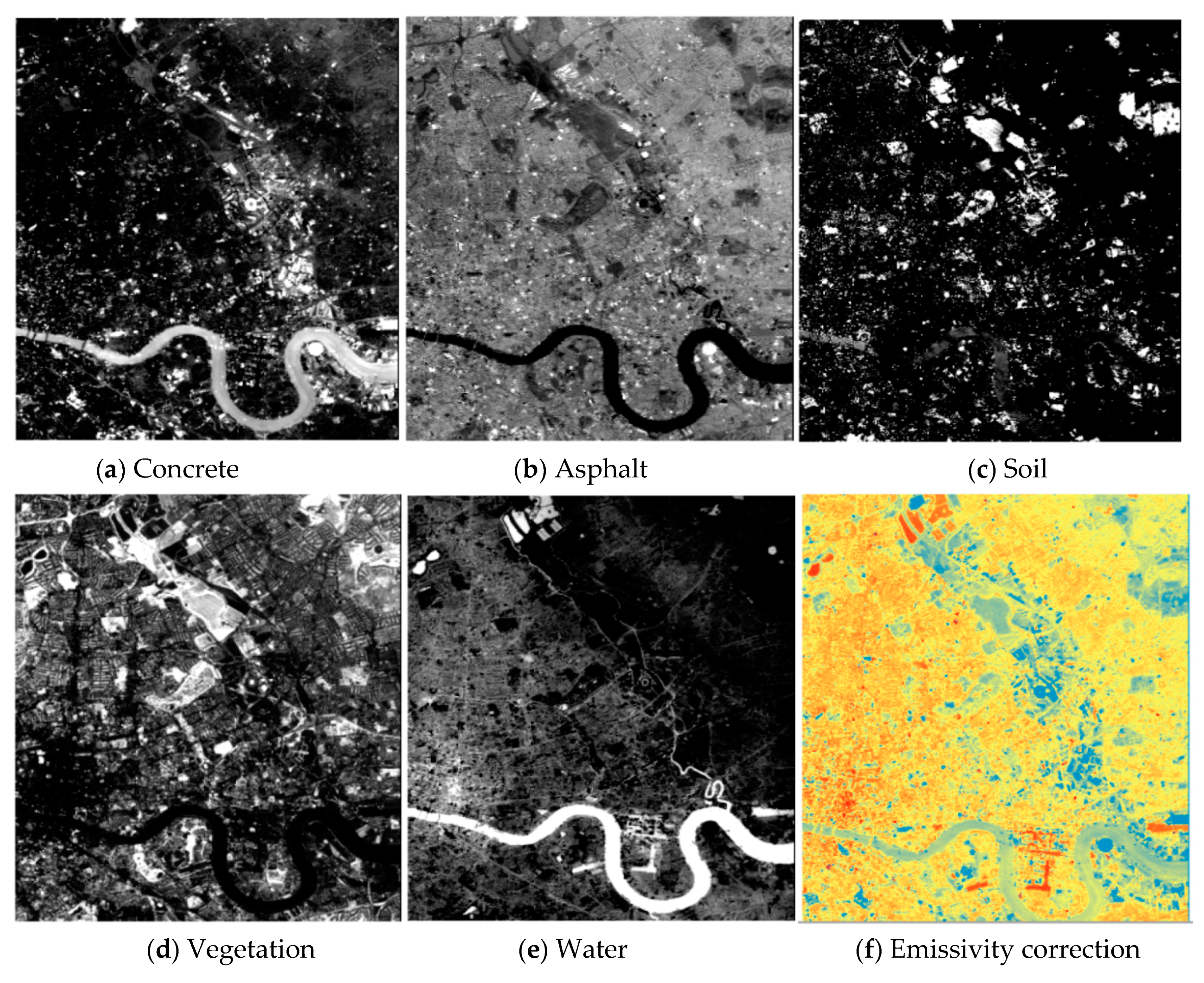
2.5. Emissivity Estimation

Emissivity can be highly variable on both sea [43] and land surfaces [44]. Emissivity from the ground is influenced by many different factors, such as variations in plant cover, water content, texture of surfaces, and viewing angle [44]. A wide range of techniques for emissivity correction were considered. Many studies have used simple approaches based on the proportion of vegetation cover, using indices such as the Normalized Difference Vegetation Index [45,46]. However, vegetation index based approaches are considered by many to be unsuitable for urban areas as they focus on the differences within vegetation classes or vegetation and soil, making them better suited to a rural environment [34,47]. Day/Night Temperature independent spectral indices were considered [48,49], but according to [41] these are unsuitable for Landsat 8 imagery, so were discounted as a common approach suitable for both OLI and ASTER was required. Thus, a land cover classification technique [50,51] was chosen as the most appropriate method for a dense urban area, based on knowledge of the study area and availability of datasets. Due to the 6 August 2015 ASTER image being a night-time scene lacking visible and SWIR bands the 15 August 2015 L1T OLI image was used for deriving the proportions of common land cover types. A manual cloud cover mask was applied to a surface reflectance corrected subset of the OLI image covering Newham in order to eliminate some areas of thin cirrus cloud that occurred in the 15 August image and could not reliably be masked using automated methods. Pure spectral signatures for key materials present on the surface within the study area were derived entirely from cloud free pixels spread across an OLI subset image covering Newham borough. It was necessary to assume that the distribution of the atmospheric effects in the unmasked areas was homogeneous. Spectral signatures for concrete, asphalt, vegetation, water, and bare soil were created in ENVI by merging representative pure pixels from across the subset image. Constrained Spectral Linear Unmixing was then used in ENVI to create fractional cover images (Figure 6a–e) for the five classes in each pixel of the image. Due to the use of archived satellite imagery it was not possible to obtain emissivity values for the five land cover classes based on simultaneous in-situ field measurements. Approximate emissivity values for each the five classes were determined following a literature search, and based on the values used by [52] and [53], as shown in Table 3. From the five land cover fractional cover images a sixth image (Figure 6f) was created containing per-pixel emissivity values based on a summation of the fractional values and chosen emissivity values for each land cover type. This per-pixel emissivity image was used for both the ASTER night-time and TIRS day-time LST image generation.

2.6. Identification of Potential Surface Urban Heat Island (SUHI) Areas

The temperature within any urban environment is highly variable, dependent upon surface materials, and many other factors [10], which underlie development of particularly hot or cold spaces. Distribution of those spaces is very important as it might increase the discomfort of human inhabitants [54]. These particularly hot or cold locations could be simply recognized by visual inspection of the LST imagery. However, this approach is highly subjective and may result in subtle patterns remaining undetected. It was decided to adopt a more quantitative approach, such as clustering techniques. Clustering is a well-established approach in determining distribution and dependencies of Surface Urban Heat Island (SUHI) development [55,56], and in [56] the authors successfully used clustering to identify both hot spots and cold spots. A wide range of spatial clustering techniques is available to determine groups of objects with similar properties [57] which can produce varied results, and can be particularly dependent on outlier values. There were no significant outliers identified by an Anselin Local Moran I test within either the ASTER or OLI LST Newham subset images, therefore, Getis-Ord Gi* was considered the most appropriate method to identify hot spots. This is a simple clustering algorithm available in ArcGIS that divides the hot spots based on the level of confidence. The distance threshold for both images was set to 90 m, i.e., one ASTER thermal pixel, and spatial relations were determined by the Fixed Distance band method, based on Euclidean Distance. The choice of distance threshold was influenced by the resampling of the ASTER image from 90 to 30 m—the spatial resolution of the Landsat 8 optical bands used in the emissivity estimate—as there was a chance that some pixels might have been affected by the much coarser initial spatial resolution.

2.7. Validation of LST Calculations

The industrial partner ARUP Engineering Consultancy Ltd. performed a surface temperature evaluation, which included the surface in the vicinity of the O2 Arena—part of the wider area of London initially processed for LST retrieval from the ASTER dataset (see Figure 7). The location of the O2 Arena was chosen due to its size, form, and ease of identification from satellite imagery. The O2 area is circular in plan with an external diameter of 365 m, with a white PTFE coated glass fiber fabric domed roof. As such it is an ideal homogeneous target of uniform surface emissivity (0.95) [58] at the spatial scale of the LST images. The evaluation was carried out using the software tools BISCO, developed by Physibel, which have the ability to calculate 2D steady-state heat transfer, using a finite element control volume energy balance method [58]. The estimation of the mean O2 Arena roof temperature accounted for absorbed radiation and heat lost by convection and re-radiation [59]. The calculation was run in accordance with the standard ISO 10211, with the parameter values outlined in Table 4.

3. Results

3.1. Emissivity Correction

The Constrained Spectral Linear Unmixing procedure applied to the Landsat 8 image produced five separate layers (represented by fraction images, Figure 6a–e), one for each land cover class. Based on those fraction images, an emissivity image (Figure 6f), was created and further included in the calculation of LST.

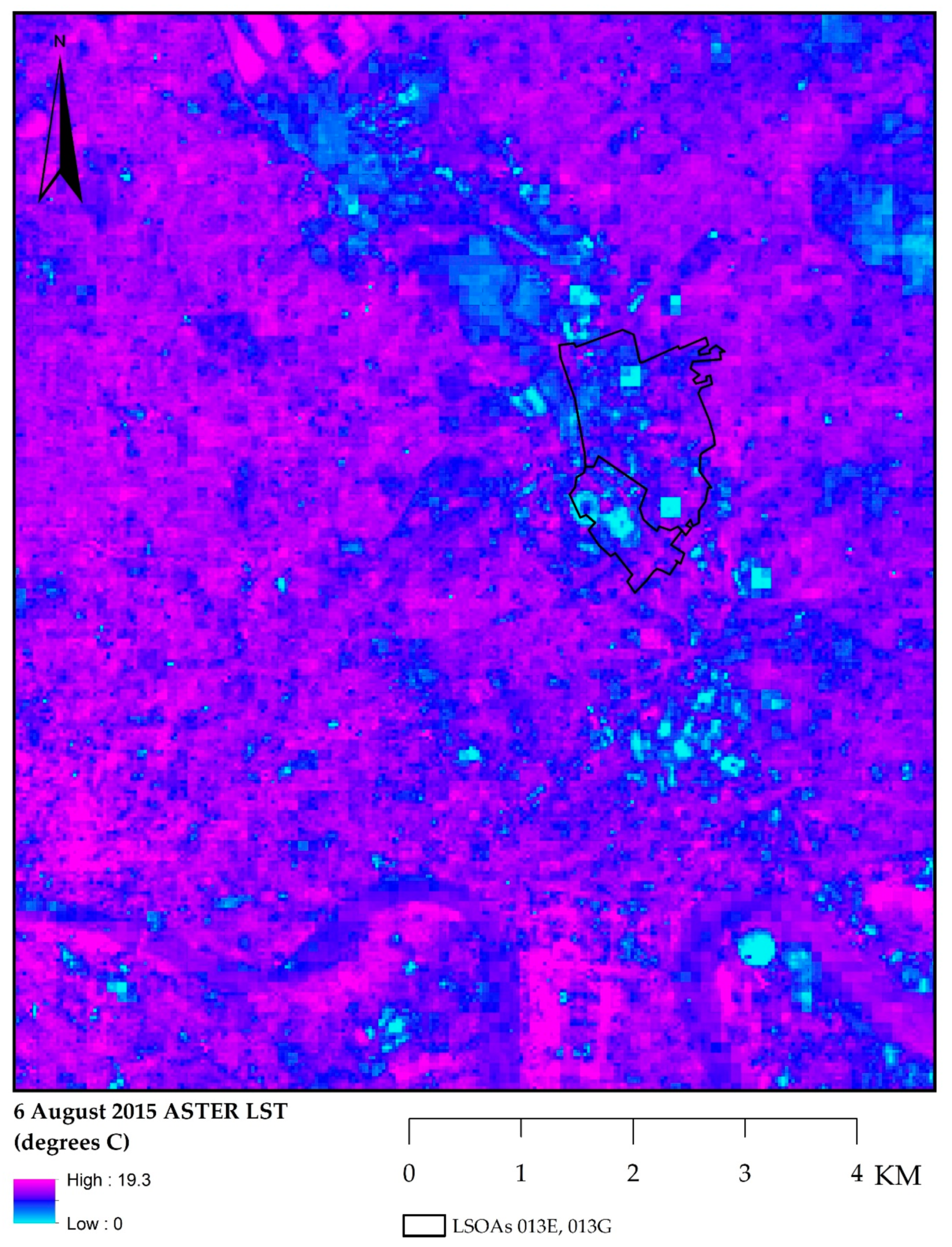
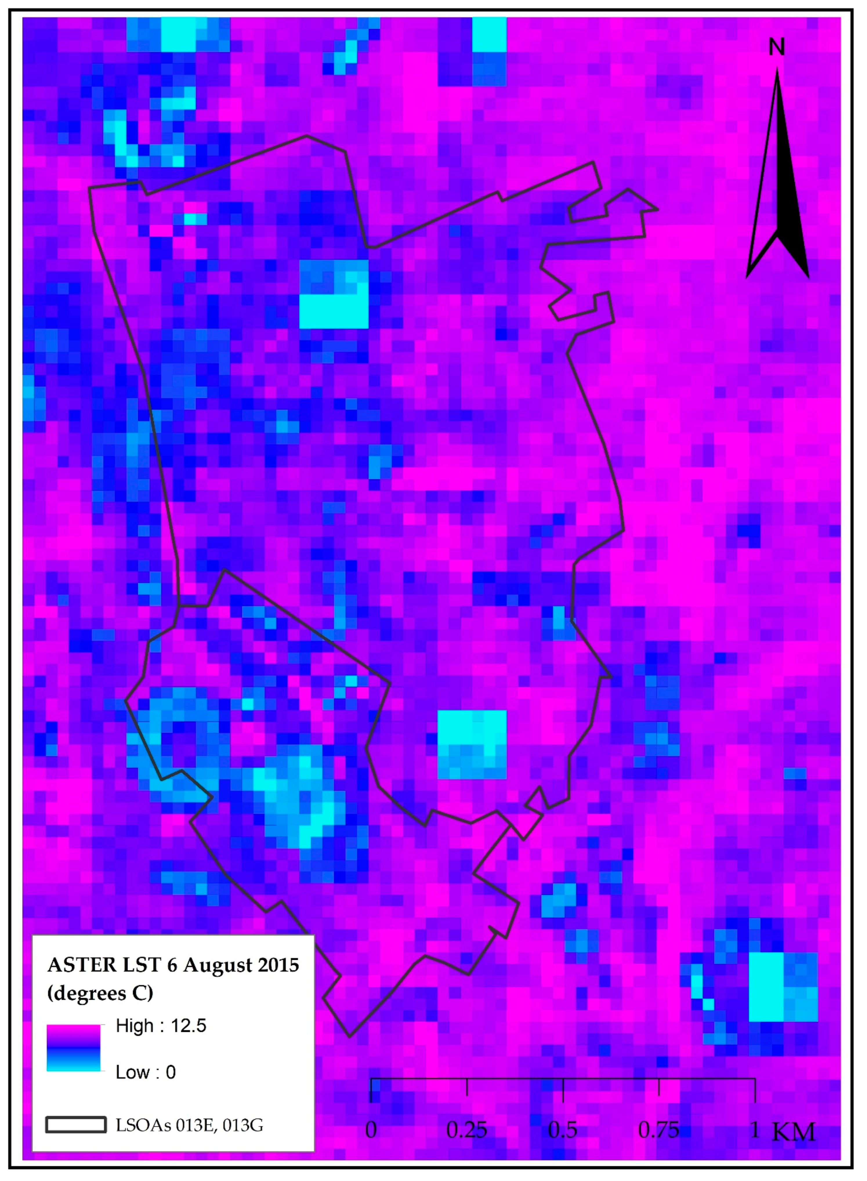
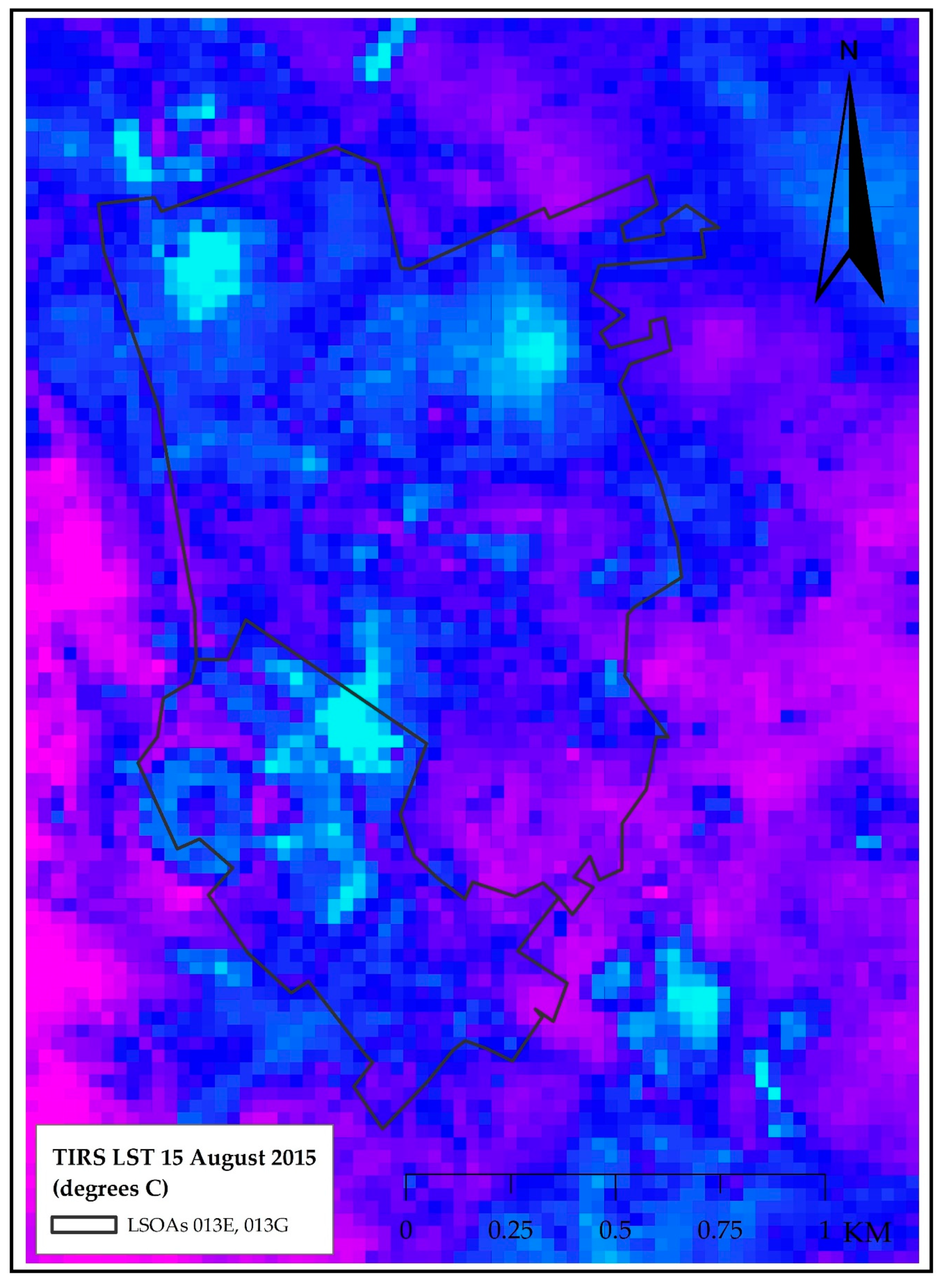
3.2. Land Surface Temperature Calculation and Validation

It was presumed that by the time of the ASTER overpass at 9:45 p.m. U.T. (10:45 p.m. local British Summer Time), rural and vegetated areas would have enough time to cool down in comparison to the densely built areas that have just started to experience an increase in emitted thermal energy. This presumption was confirmed by the results of LST calculation (Figure 7 shows the boundaries of the two LSOAs used for better orientation). The calculated thermal range was 0–19.3 °C. This study was primarily interested in the investigation of LST over newly built areas of Stratford, previously identified by the LSOAs 013E and 013G (Figure 4). The extent of spatial thermal distribution is visualized within the context of these LSOAs in Figure 8 for ASTER and Figure 9 for Landsat 8 TIRS. The main orientation point can be seen in the form of the oval shaped Olympic Stadium on the South West boundary, which was one of the coldest parts due to the cooling caused by the presence of a large grass area in its vicinity.
The results of night-time ASTER and day-time Landsat 8 LST thermal models were interpreted with regard to the different overpass times but cannot be directly compared due to temporal inconsistency. However, the expected cooling and warming trends within the non-vegetated and vegetated environments were clearly depicted. The ASTER thermal model (Figure 8) shows that the warmest parts of the image are urbanized spaces. Green vegetated areas are the coldest, supporting thermal trends described elsewhere by [10] and [30]. Within the thermal model for day-time Landsat 8 imagery (Figure 9) densely urbanized parts located to the West outside the LSOA boundaries warmed up very quickly. However, vegetated areas are still quite cool, displayed as the coldest.
The project partners ARUP Engineering Consultancy Ltd. compared their directly measured results from the ASTER overpass time with the Land Surface Temperature calculation derived by this study from satellite imagery using the Split Window algorithm. With a low Convective Heat Transfer Coefficient their mean average temperature value (5.2 °C) for the O2 Arena roof was determined to be almost identical to the ASTER-derived value [58], within the precision limits of the satellite dataset. The mean average temperature calculated by remote sensing methods for those ASTER pixels contained wholly within the 365 m diameter the O2 Arena roof was 5.08 °C. Figure 10 shows the visual results for the roof cross-section.
From Figure 7 it can clearly be seen that vegetated areas are coldest, represented by the bright blue color scheme and areas of densely build urban environment are depicted as warmest—displayed in purple color scheme, as well as shallow parts of river Thames with its densely built river banks, whose distinctive shape is clearly recognizable. Isle of Dogs is also one of the warmest parts as it contains Canary Wharf, which is dominated by high rise buildings and non-vegetated surfaces. Figure 8 and Figure 9 show the boundaries of LSOAs 13G and 13E overlain on ASTER and TIRS LST images respectively. The main landmark as an orientation point can be also seen in the form of the oval shaped Olympic Stadium on the South West boundary, which came out as one of the coldest parts. Figure 8 and Figure 9 show the expected general trends for the times of day, but to reliably identify thermal spatial patterns clustering analysis was necessary.

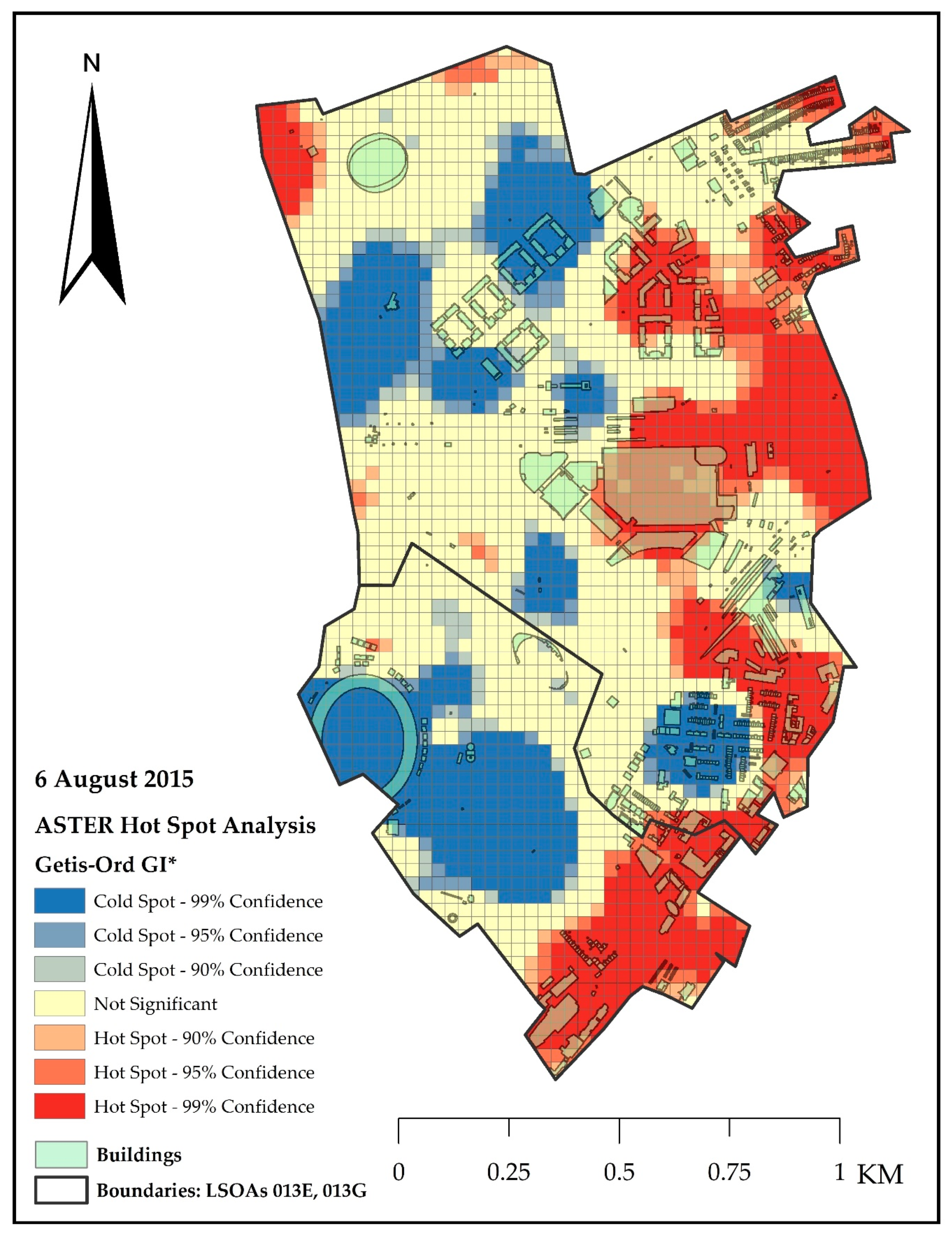
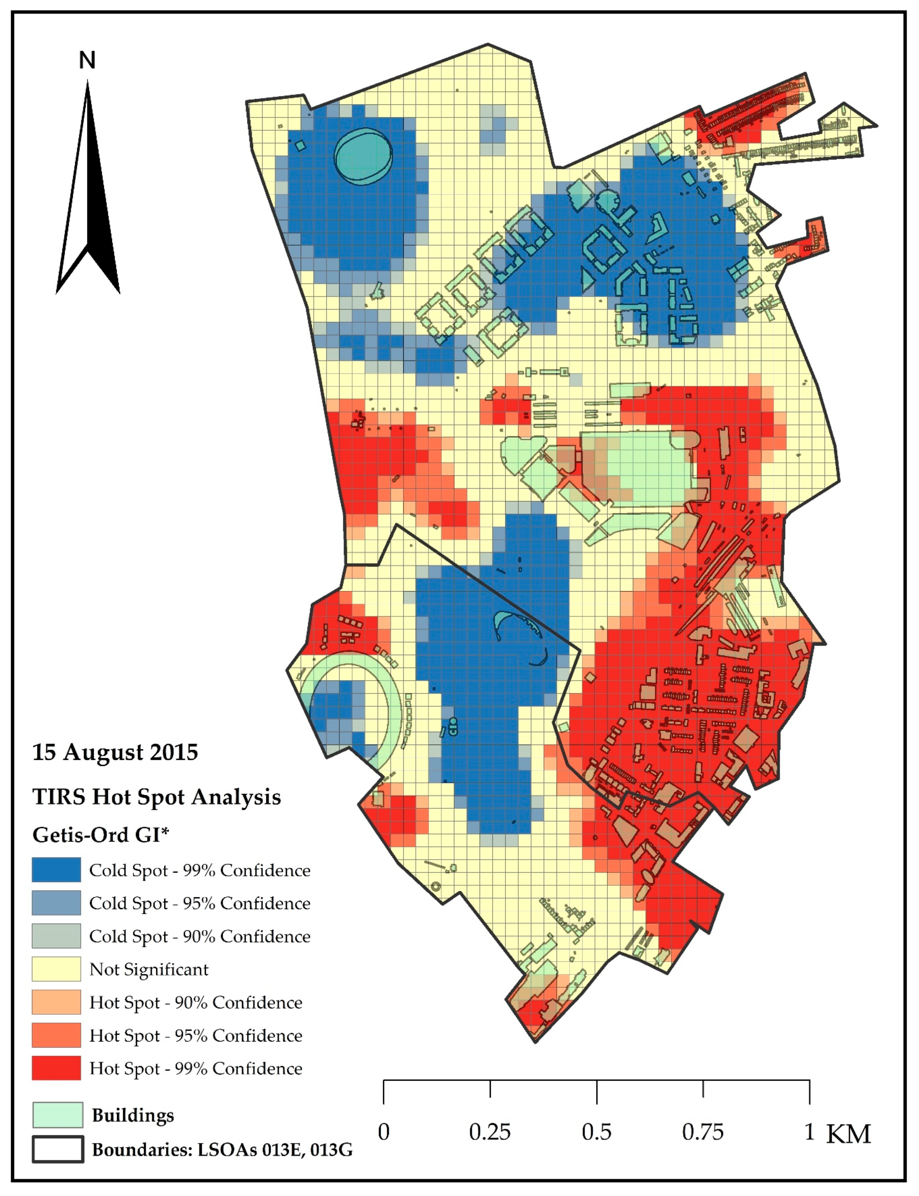
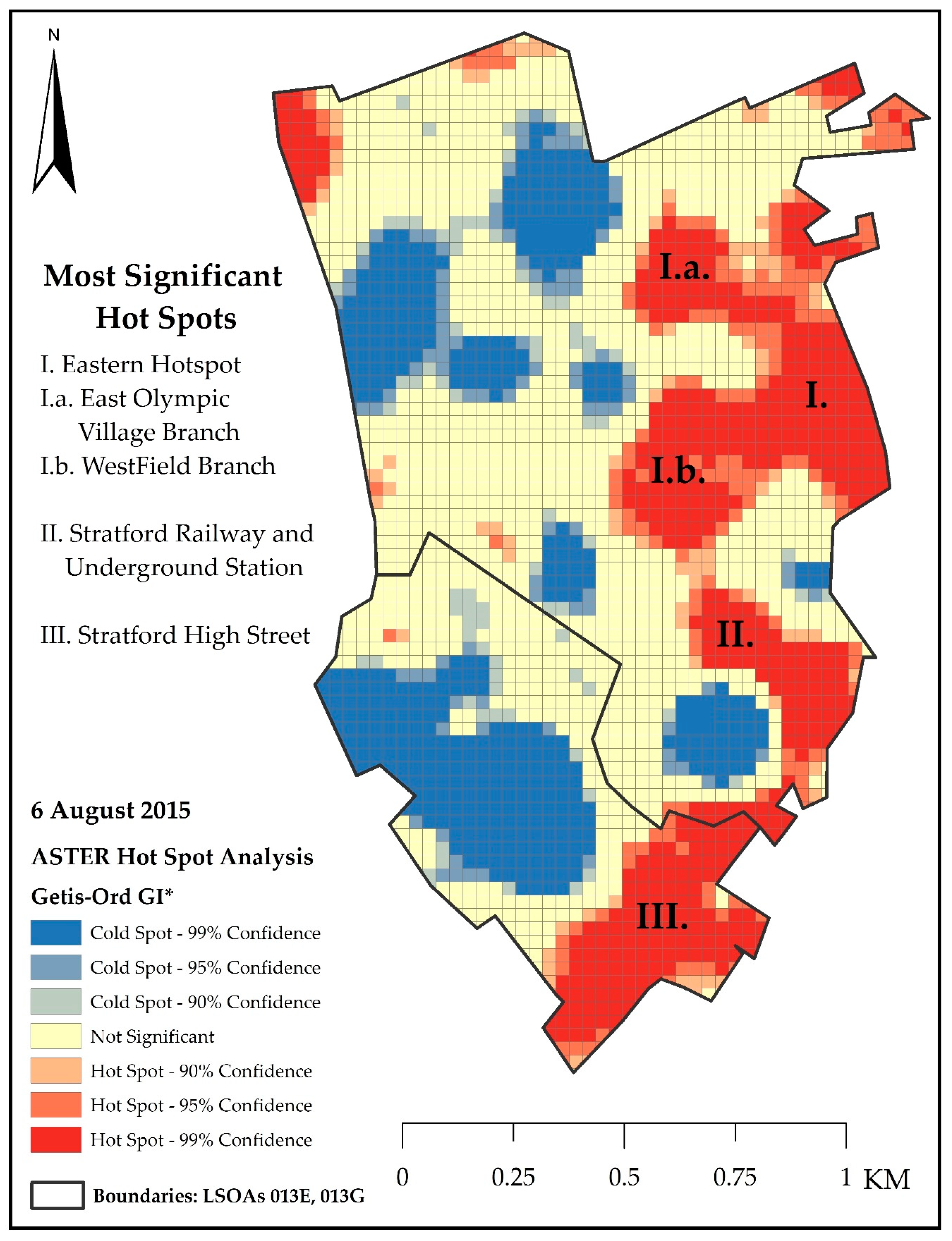
3.3. Identification of Potential Surface Urban Heat Island (SUHI) Areas

Getis-Ord-Gi* cluster analysis provided the basis for interpretation of spatial thermal patterns from both ASTER and TIRS satellite images (Figure 11 and Figure 12). The differences in thermal emissivity are the most recognizable in the night-time ASTER imagery; therefore results of ASTER based cluster analysis offered an important basis for the identification of SUHIs (Figure 11). As a result, three main clusters and two branches were identified, based upon the 90% confidence level: Eastern hot spot (East Olympic Village and Westfield branch), Stratford Railway and Underground station, and Stratford High Street hot spot (Figure 13). In a wider context these are probably sub-components of one big cluster. For better orientation the building polygon overlay is included in Figure 11 and Figure 12. Some hot spots depicted in the ASTER hot spot image (Figure 11) are not present on the Landsat 8 hot spot map (Figure 12), including the East Olympic Village and South part of Stratford High Street. Conversely, some day-time hot spots from Landsat 8 (Figure 12) are not depicted by the ASTER hot spot map (Figure 11), such as the central West area. Figure 11 shows that the Western part of the East Olympic Village is located on the border of ASTER cold and hot spots. However, these two clusters are different, they are very close to each other, divided only by a road. Buildings in this location are the same type and age. The Central and Eastern parts of Eastern Olympic Village are completely located within the hot spot I.a (Figure 13). The old residential parts on the Eastern edge of the area are also part of the hot spot, with a confidence level of 99%. The Eastern Olympic Village is particularly interesting as the whole area was built recently and there were no old residential buildings mixed within the main village, only the old buildings on the Eastern edge, suggesting that thermal performance of the new built area is comparable to the older buildings to the East, despite the improvements in building materials and building design. Overall East Olympic Village can be considered as a homogenous area, confirmed by field inspection prior to the remote sensing analysis, and its presence within a hot spot could not have been explained by indirect methods. Another very significant hot spot was identified in the location of Westfield Stratford City, which is a major shopping mall (hot spot I.b. in Figure 13) and the busiest part of the study area in the day-time, with a lot of anthropogenic heat generated in addition to heat from the neighboring railway and road traffic. The same situation was recorded west from the old Stratford rail station (hot spot II in Figure 13), which is a very busy railway junction. A third cluster was identified on Stratford High Street (hot spot III in Figure 13), which contained newly built buildings mixed up with old residential and retail properties and which experienced a large increase in road traffic during the 2010–2015 study period.

4. Discussion

4.1. Identification of Newly Built Areas

The choice of most recent period 2010–2015 was based on the presumption that it contained the newest buildings; that provided the highest chance they were built out of modern materials using more sustainable methods. However, this assumption required validation by separate research. Unfortunately, in the United Kingdom the year of build is not adequately recorded nor freely accessible, unlike in some European Union member states. The initial intention to analyze residential together with commercial/industrial buildings, to ensure more realistic representation, proved to be impossible as the available temporal coverage of the dataset containing the age of Commercial and Industrial stock only extended until 2003 [60]. As a result, the identification of study areas was solely based on the residential dwelling dataset at the finest scale available, LSOAs.

4.2. Calculation of Land Surface Temperature (LST)

Spatial resolution of the thermal bands of available satellite remote sensors is considerably coarser than is ideal for urban LST monitoring. For the London area, aerial thermal data were available from Bluesky International Ltd., with a spatial resolution of 50 cm. Such spatial resolution would greatly improve the accuracy of LST modelling. Unfortunately, the BlueSky data only covered roughly 2% of the study area and considering the most recent available dates are from 2013, would not fit the purpose of the study, which requires freely available regularly updated imagery. As historical records related to the amounts of water vapor and absorption were not available, a simplified version of the Split Window algorithm containing only the estimation of transmittance and emissivity [38] was used. The amount of water vapor is not considered to be constant for particular atmospheric profiles, as it is in the case of O3 and CO2 [39], therefore, more a complex approach to water vapor retrieval from MODIS should be adopted where possible in the future during the transmittance estimate. Meteorological data were retrieved from the nearest available meteorological station, approximately 10.5 km away. This station was also situated in parkland rather than a dense urban environment, which consequently increased the uncertainty of transmittance estimation. The temporal difference between the night-time ASTER image and the day-time Landsat 8 image used in emissivity estimation was only 9 days. This was short enough to safely assume there was no significant change in land cover during this period. More significant impact was related to the presence of a thin veil of Cirrus clouds recorded over some places. To ensure the optimal results during image classification, spectral signatures were taken only from cloud-free areas. Despite the fact that the Split Window algorithm is not advised by [37] for Landsat 8 imagery, due to the calibration uncertainty in band 11 of TIRS data, the Landsat 8 image was investigated in the same manner as the ASTER image, which ensured methodological consistency.

4.3. Identification of Potential Surface Urban Heat Island (SUHI) Areas

Although the ArcMap Getis-Ord Gi* statistics tool proved to be sufficient, other available scientific methods should be reviewed in the future. Three main clusters were identified (Figure 13), but particularly interesting were the East Olympic Village branch and Westfield branch (for wider context see Figure 11 and Figure 12). With the exception of the East Olympic Village and Westfield Stratford City mall, other clusters were not homogenous in regard to the building age as new buildings were mixed with older ones. As Westfield is considered to be the busiest area during the day-time, the presence of a hot spot can be potentially explained by the accumulation of anthropogenic heat in the densely urbanized areas caused by heating, cooling, transportation, or heat produced by human bodies [61]. Field examination within East Olympic Village proved that this location consisted of relatively homogenous buildings within the same period of build, with the low level of traffic, surrounded by trees, green spaces, and green rooftops on some buildings (Figure 14a).
The Western part of this location was clearly outside the UHI cluster, but its Eastern part was included within (Figure 14b). Its most Eastern part was in the vicinity of rail tracks bordering partially with a parking area and an area of unknown use, constructed out of asphalt and concrete, and further to the East was an old residential development. This might have potentially caused the inclusion of its Eastern part within the UHI cluster. The presumption that green rooftops can influence the cooling process at street level is considered to be valid only when buildings are up to 10 m tall [62]. All buildings in this location with green rooves are higher than 10 m (Figure 5 and Figure 14), and do not appear to exert any cooling influence in the hot spot maps. Due to the complexity of influencing factors it would be advisable to model urban canyons in separate research as well as to conduct further detailed analysis of materials used during the construction process—mainly claddings used for facades.

5. Conclusions

Overall this study has proven that remote sensing methods using freely available satellite thermal imagery from ASTER and Landsat 8 are not only reliable for UHI investigations in a wide context, but are also capable of identifying thermally problematic localized new developments within the challenging atmospheric and climatic conditions of London, despite limited spatial and spectral resolution. Within the two LSOAs that experienced the greatest amount of new residential buildings in the period 2010–2015 it was possible to identify through hot spot analysis three locations of new urban development where thermal hot spots appear to have been created, and for which mitigation measures should be considered by local planners. The new residential buildings in these locations were constructed out of smart materials with sustainability in mind, suggesting that planning at a landscape-level was not adequate to ensure a comfortable thermal regime despite the consideration given to sustainable design of individual building. This work paves the way for further cost-effective satellite-based thermal analysis to influence the planning of new developments, and long-term monitoring of existing developments in London and elsewhere. Further wide-scale development in the form of a new cultural hub [63,64] is currently under way at Stratford, which will significantly affect the future distribution of green spaces, and consequently influence their cooling ability, further exacerbating the thermal stress that this area of London is already experiencing. It is recommended that a similar approach be adopted in future housing development plans to characterize thermal patterns throughout London and similar cities under pressure for new housing developments, and provide a baseline for time-series monitoring.
Although the inclusion of the East Olympic Village within the hot spot cluster requires more investigation, significant thermal effects could be due to the orientation of the urban canyons, prevailing winds within them, or building materials used. Further detailed canyon modelling is advised. This ought to consider different wind patterns and detailed investigation of materials used, including their thermal properties, as different types and colors of facade cladding were confirmed during field investigation. During the period 2010–2015 development in London was mainly focused on the construction of residential buildings, due to the high housing demands resulting from increasing population. Although this justifies the choice of dataset used in the quantitative analysis for this study, ideally it would be recommended to include the age groups and counts for commercial/industrial building, if available, in any future analysis to better reflect the overall situation.
The biggest challenge during the calculation of LST was the current availability of suitable satellite imagery. This was not ideal, due to available spatial and spectral resolution and the issues of cloudiness and humidity in London. Despite the limitations imposed by available datasets independent validation performed by ARUP [58] has confirmed the LST model produced results of acceptable accuracy both with Landsat 8 and ASTER imagery. Incorporation of Landsat 8 imagery into the emissivity correction for the ASTER dataset could influence the accuracy of LST calculation. For any future investigation of LST over this particular location it would be advisable to obtain measurements of water vapor and incorporate a carefully considered atmospheric model into the estimation of emissivity in order to obtain optimal results. Incorporation of satellite remote sensing and GIS into future planning of London urban development is highly recommended, including the further investigation of technologically advanced building materials with improved thermal properties, distribution of green spaces and shaded areas, and capability to maintain desired airflow.

Author Contributions

Conceptualization, D.M. and M.W.; Methodology, D.M. and M.W.; Software, M.W.; Validation, D.M.; Formal analysis, D.M.; Investigation, D.M.; Resources, D.M and M.W.; Data curation, D.M.; Writing—original draft preparation, D.M and M.W.; Writing—review and editing, M.W.; Visualization, D.M.; Supervision, M.W.; Project administration, M.W.

Funding

This research received no external funding.

Acknowledgments

The authors gratefully acknowledge project partners ARUP Engineering Consultancy Ltd., London, UK, with special thanks to Mattia Donato.

Conflicts of Interest

The authors declare no conflict of interest.

References

  1. Barlow, J.F.; Halios, C.H.; Lane, S.E.; Wood, C.R. Observations of urban boundary layer structure during a strong urban heat island event. Environ. Fluid Mech. 2015, 15, 373–398. [Google Scholar] [CrossRef]
  2. Zhang, Y.; Cheng, J. Spatio-Temporal Analysis of Urban Heat Island Using Multisource Remote Sensing Data: A Case Study in Hangzhou, China. IEEE J. Sel. Top. Appl. Earth Obs. Remote Sens. 2019. [Google Scholar] [CrossRef]
  3. Voogt, J.A.; Oke, T.R. Thermal remote sensing of urban climates. Remote Sens. Environ. 2003, 86, 370–384. [Google Scholar] [CrossRef]
  4. Palme, M.; Inostroza, L.; Villacreses, G.; Lobato-Cordero, A.; Carrasco, C. From urban climate to energy consumption. Enhancing building performance simulation by including the urban heat island effect. Energy Build. 2017, 145, 107–120. [Google Scholar] [CrossRef]
  5. Oke, T.R. The heat island of the urban boundary layer: Characteristics, causes and effects. Wind Clim. Cities 1995, 277, 81–107. [Google Scholar] [CrossRef]
  6. Voogt, J.A.; Oke, T.R. Complete urban surface temperatures. J. Appl. Meteorol. 1997, 36, 117–1132. [Google Scholar] [CrossRef]
  7. Rao, P.K. Remote sensing of urban heat islands from an environmental satellite. Bull. Am. Meteorol. Soc. 1972, 53, 647–648. [Google Scholar]
  8. Zhou, D.; Xiao, J.; Berger, C.; Deilami, K.; Zhou, Y.; Frolking, S.; Yao RQiao, Z.; Sobrino, J.A. Satellite Remote Sensing of Surface Urban Heat Islands: Progress, Challenges, and Perspectives. Remote Sens. 2018, 11, 48. [Google Scholar] [CrossRef]
  9. Koomen, E.; Diogo, V. Assessing potential future urban heat island patterns following climate scenarios, socio-economic developments and spatial planning strategies. Mitig. Adapt. Strateg. Glob. Chang. 2017, 22, 287–306. [Google Scholar] [CrossRef]
  10. Oke, T.R. The energetic basis of the urban heat island. Quart. J. R. Meteorol. Soc. 1982, 108, 1–24. [Google Scholar] [CrossRef]
  11. Ichinose, T.; Shimodozono, K.; Hanaki, K. Impact of anthropogenic heat on urban climate in Tokyo. Atmos. Environ. 1999, 33, 3897–3909. [Google Scholar] [CrossRef]
  12. Watkins, R. The Impact of the Urban Environment on the Energy Used for Cooling Buildings. Ph.D. Thesis, Brunel University, Uxbridge, London, UK, 2002. Available online: http://citeseerx.ist.psu.edu/viewdoc/download?doi=10.1.1.425.8093&rep=rep1&type=pdf (accessed on 2 September 2019).
  13. Eliasson, I.; Svensson, M.K. Spatial air temperature variations and urban land use—Statistical approach. Meteorol. Applic. 2013, 10, 135–149. [Google Scholar] [CrossRef]
  14. Oke, T.R. Canyon Geometry and the Nocturnal Urban Heat-Island—Comparison of Scale Model and Field Observations. Int. J. Climatol. 1981, 1, 237–254. [Google Scholar] [CrossRef]
  15. Collier, C.G. The impact of urban areas on weather. Quart. J. R. Meteorol. Soc. 2006, 132, 1–25. [Google Scholar] [CrossRef]
  16. Alexander, J.; Daw, P.; Denig, S.; Owens, W.; Richards, D.; Trimble, E.; Verdis, S. Our Urban Future. In The Crystal: A Sustainable Cities Initiative by Siemens; Booklink: Slovenia, Balkans, 2003. [Google Scholar]
  17. Mayor of London. Smart London Plan. 2013. Available online: http://www.london.gov.uk/sites/default/files/smart_london_plan.pdf (accessed on 2 September 2019).
  18. Mayor of London. 2016. The Future of Smart—Update report of the smart London Plan. 2013. Available online: https://www.london.gov.uk/sites/default/files/gla_smartlondon_report_web_4.pdf (accessed on 2 September 2019).
  19. Construction Industry Council. CITB: Impact of the Recession on Construction Professional Services. 2018. Available online: https://www.citb.co.uk/research-insight/research-reports/impact-of-the-recession-on-construction-professional-services/ (accessed on 2 September 2019).
  20. Mills, G. Luke Howard and the climate of London. Weather 2008, 63, 153–157. [Google Scholar] [CrossRef]
  21. Kolokotroni, M.; Giridharan, R. Urban heat island intensity in London: An investigation of the impact of physical characteristics on changes in outdoor air temperature during summer. Sol. Energy 2008, 82, 986–998. [Google Scholar] [CrossRef] [Green Version]
  22. Giridharan, R.; Kolokotroni, M. Urban Heat island characteristics in London during winter. Sol. Energy 2009, 83, 1668–1682. [Google Scholar] [CrossRef]
  23. Kolokotroni, M.; Davies, M.; Croxford, B.; Bhuiyan, S.; Mavrogianni, A. A validated methodology for the prediction of heating and cooling energy demand for buildings within the urban heat island: Case-study of London. Sol. Energy 2010, 84, 2246–2255. [Google Scholar] [CrossRef]
  24. Shahrestani, M.; Yao, R.; Luo, Z.; Turkbeyler, E.; Davies, H. A field study of urban microclimates in London. Renew. Energy 2015, 73, 3–9. [Google Scholar] [CrossRef] [Green Version]
  25. Zhou, B.; Lauwaet, D.; Hooyberghs, H.; De Ridder, K.; Kropp, J.P.; Rybski, D. Assessing Seasonality in the Surface Urban Heat Island of London. J. Appl. Meteorol. Climatol. 2015, 55, 493–505. [Google Scholar] [CrossRef]
  26. The National Archives. Office for National Statistics—Super Output Area (SOA). Available online: http://webarchive.nationalarchives.gov.uk/20160105160709/http://www.ons.gov.uk/ons/guide-method/geography/beginner-s-guide/census/super-output-areas--soas-/index.html (accessed on 2 September 2019).
  27. NASA. NASA Landsat Science, Landsat 7. Available online: http://landsat.gsfc.nasa.gov/?p=3184 (accessed on 2 September 2019).
  28. NASA. Jet Propulsion Laboratory. Aster Advanced Spaceborne Thermal Emission and Reflection Radiometer. Available online: http://asterweb.jpl.nasa.gov/mission.asp (accessed on 31 July 2019).
  29. NASA. NASA Landsat Science, Landsat 8. Available online: http://landsat.gsfc.nasa.gov/?p=3186 (accessed on 2 September 2019).
  30. Haeger-Eugensson, M.; Holmer, B. Advection caused by the urban heat island circulation as a regulating factor on the nocturnal urban heat island. Int. J. Climatol. 1999, 19, 975–988. [Google Scholar] [CrossRef]
  31. Abrams, M.; Hook, S. Jet Propulsion Laboratory—Aster Users Handbook. 2002. Available online: https://asterweb.jpl.nasa.gov/content/03_data/04_Documents/aster_user_guide_v2.pdf (accessed on 2 September 2019).
  32. Ghulam, A. How to Calculate Reflectance and Temperature Using ASTER Data. 2009. Available online: http://www.pancroma.com/downloads/ASTER%20Temperature%20and%20Reflectance.pdf (accessed on 2 September 2019).
  33. Chander, G.; Markham, B.L.; Helder, D.L. Summary of current radiometric calibration coefficients for Landsat MSS, TM, ETM+ and EO-1 ALI sensors. Remote Sens. Environ. 2009, 117, 893–903. [Google Scholar] [CrossRef]
  34. Jimenez-Munoz, J.C.; Sobrino, J.A. A Single–Channel Algorithm for Land–Surface Temperature Retrieval from Aster Data. IEEE Geosci. Remote Sens. Lett. 2010, 7, 176–179. [Google Scholar] [CrossRef]
  35. Price, J.C. Land Surface temperature measurements from the split window channels of the NOAA 7 Advanced Very High Resolution Radiometer. J. Geophys. Res. Atmos. 1984, 89, 7231–7237. [Google Scholar] [CrossRef]
  36. Qin, Z.; Olm, G.D.; Karnelier, A.; Berliner, P. Derivation of split window algorithm and its sensitivity analysis for retrieving land surface temperature from NOAA-AVHRR—Advanced very high resolution radiometer data. J. Geophys. Res. 2001, 106, 1984–2012. [Google Scholar] [CrossRef]
  37. Barsi, J.A.; Schott, J.R.; Hook, S.J.; Raqueno, N.G.; Markham, B.L.; Radocinski, R.G. Landsat-8 Thermal Infrared Sensor (TIRS) Vicarious Radiometric Calibration. Remote Sens. 2014, 6, 11607–11626. [Google Scholar] [CrossRef] [Green Version]
  38. Qin, Z.; Li, W.; Gao, M.; Zhang, H. An algorithm to retrieve land surface temperature from ASTER thermal band data for agricultural drought monitoring. SPIE Int. Soc. Opt. Eng. 2006, 6359. [Google Scholar] [CrossRef]
  39. Sobrino, J.A.; Coll, C.; Caselles, V. Atmospheric correction of land surface temperature using NOAA-11 AVHRR channels 4 and 5. Remote Sens. Environ. 1991, 38, 19–34. [Google Scholar] [CrossRef]
  40. Rozenstein, O.; Qin, Z.; Derimian, Y.; Karnieli, A. Derivation of Land Surface Temperature for Landsat 8 TIRS using a Split Window Algorithm. Sensors 2014, 14, 5768–5780. [Google Scholar] [CrossRef]
  41. Yu, X.; Guo, X.; Wu, Z. Land Surface Temperature Retrieval from Landsat 8 TIRS—Comparison between Radiative Transfer Equation—Based Method, Split Window Algorithm and Single Channel Method. Remote Sens. 2014, 2014, 9829–9852. [Google Scholar] [CrossRef]
  42. Rp5.co.uk. Weather Archive in London/St. James’s Park—Dataset. 2016. Available online: http://rp5.co.uk/Weather_archive_in_London,_St._James's_Park (accessed on 2 September 2019).
  43. Cheng, J.; Cheng, X.; Meng, X.; Zhou, G. A Monte Carlo Emissivity Model for Wind-Roughened Sea Surface. Sensor 2019, 19, 2166. [Google Scholar] [CrossRef]
  44. Salisbury, J.W.; D’Aria, D.M. Emissivity of terrestrial materials in the 8-14 µm atmospheric window. Remote Sens. Environ. 1992, 42, 83–106. [Google Scholar] [CrossRef]
  45. Van de Griend, A.A.; Owe, M. On the relationship between thermal emissivity and the normalized difference vegetation index for natural surfaces. Int. J. Remote Sens. 1993, 14, 1119–1131. [Google Scholar] [CrossRef]
  46. Valor, E.; Caselles, V. Mapping land surface emissivity from NDVI. Application to European, African and South American areas. Remote Sens. Environ. 1996, 57, 167–184. [Google Scholar] [CrossRef]
  47. Lin, L.; Zhang, Y. Urban Heat Island Analysis Using the Landsat TM Data and Aster Data: A case study in Hong Kong. Remote Sens. 2011, 3, 1535–1552. [Google Scholar] [CrossRef]
  48. Becker, F.; Li, Z.-L. Surface temperature and emissivity at various scales: Definition, Measurements and related problems. Remote Sens. Rev. 1995, 12, 225–253. [Google Scholar] [CrossRef]
  49. Wan, Z.; Li, Z.-L. A land surface temperature measurement from EOS/MODIS data. 1997. Available online: http://modis.gsfc.nasa.gov/MODIS/LAND/REPORTS/wan.1997.4.pdf (accessed on 2 September 2019).
  50. Gillespie, A.; Rokugawa, S.; Matsunaga, T.; Kahle, A.B. A Temperature and emissivity separation algorithm for advanced spaceborne thermal emission and reflection radiometer (ASTER) images. IEEE Trans. Geosci. Remote Sens. 1998, 36, 1113–1126. [Google Scholar] [CrossRef]
  51. Peres, L.F.; DaCamara, C.C. Emissivity maps to retrieve land-surface temperature from MSG/SEVIRI. IEEE Trans. Geosci. Remote Sens. 2005, 43, 1834–1844. [Google Scholar] [CrossRef]
  52. Kotthaus, S.; Smith, T.E.L.; Wooster, M.J.; Grimmond, C.S.B. Derivation of an urban materials spectral library through emittance and reflectance spectroscopy. ISPRS J. Photogramm. Remote Sens. 2014, 94, 194–212. [Google Scholar] [CrossRef] [Green Version]
  53. Ogawa, K.; Schmugge, T.; Jacob, F.; French, A. Estimation of broadband emissivity from satellite multi-channel thermal infrared data using spectral libraries. Agron. EDP Sci. 2002, 22, 695–696. [Google Scholar] [CrossRef]
  54. Majumdar, D.D.; Biswas, A. Quantifying land surface temperature change from LISA clusters: An alternative approach to identifying urban land use transformation. Landsc. Urb. Plan. 2013, 153, 51–65. [Google Scholar] [CrossRef]
  55. Buyantuyev, A.; Wu, J. Urban heat islands and landscape heterogeneity: Linking spatiotemporal variation in surface temperature to land-cover and socioeconomic patterns. Landsc. Ecol. 2010, 25, 17–33. [Google Scholar] [CrossRef]
  56. Guo, G.; Wu, Z.; Xiao, R.; Chen, Y.; Xiaonan, L.; Zhang, X. Impacts of urban biophysical composition on land surface temperature in urban heat island clusters. Landsc. Urb. Plan. 2015, 135, 1–10. [Google Scholar] [CrossRef]
  57. Estivill-Castro, V.; Lee, I. AMOEBA: Hierarchical clustering based on spatial proximity using Delaunay diagram. In Proceedings of the 9th International Symposium on Spatial Data Handling, Beijing, China, 10–12 August 2000. [Google Scholar]
  58. Donato, M.; (Arup Engineering Consultants, London, UK). Arup project briefing 2 September 2010. Personal communication, 2016, unpublished. [Google Scholar]
  59. Lienhard, J., IV; Lienhard, V.J. A Heat Transfer Textbook, 4th ed.; Phlogiston Press: Cambridge, MA, USA, 2016; 766p. [Google Scholar]
  60. Department for Communities and Local Government (DCLG—gov.uk). Age of Commercial and Industrial Stock. 2004. Available online: https://www.gov.uk/government/statistical-data-sets/live-tables-on-commercial-and-industrial-floorspace-and-rateable-value-statistics (accessed on 2 September 2019).
  61. Flanner, M.G. Integrating anthropogenic heat flux with global climate models. Geophys. Res. Lett. 2009, 36. [Google Scholar] [CrossRef] [Green Version]
  62. Wong, N.H.; Chen, Y.; Ong Ch, L.; Sia, A. Investigation of thermal benefits of rooftop garden in the tropical environment. Build. Environ. 2003, 38, 261–270. [Google Scholar] [CrossRef]
  63. Mayor of London, Mayor of London—London Assembly, Mayor Announces Major New Plans for East London. 2016. Available online: https://www.london.gov.uk/press-releases-6230 (accessed on 2 September 2019).
  64. Queen Elizabeth Olympic Park. New Images Released for Stratford Waterfront Show Detailed Designs. 2016. Available online: http://www.queenelizabetholympicpark.co.uk/media/press-releases/2016/07/new-images-released-for-stratford-waterfront-show-detailed-designs (accessed on 2 September 2019).
Figure 1. Causality of Urban Heat Islands (UHIs) development (based on works published by [1,3]).
Remotesensing 11 02244 g001
Figure 2. Map of London boroughs residential development in years 2010–2015 (Lower Super Output Area (LSOA) subdivision). LSOAs 013G and 013E within Newham borough are highlighted in blue. Contains National Statistics data © Crown copyright and database right (2015) and (2012). Contains Ordnance Survey data © Crown copyright and database right (2015) and (2012).
Remotesensing 11 02244 g002
Figure 3. The 11 LSOAs with the greatest number of new residential buildings built in London between 2010 and 2015. Contains National Statistics data © Crown copyright and database right (2015) and (2012). Contains Ordnance Survey data © Crown copyright and database right (2015) and (2012).
Remotesensing 11 02244 g003
Figure 4. Map showing the number of new buildings 2010–2015 per LSOAs within the boundaries of Newham borough. The chosen LSOAs 013E and 013G are outlined. Contains National Statistics data © Crown copyright and database right (2015) and (2012). Contains Ordnance Survey data © Crown copyright and database right (2015) and (2012).
Remotesensing 11 02244 g004
Figure 5. The 50 cm spatial resolution Digital Surface Model (DSM). Contains Ordnance Survey data © Crown Copyright and database right (2012). Contains Royal Mail data © Royal Mail copyright and database right (2012). Contains bathymetry data by GEBCO © Copyright (2012). Contains data by Land and Property Services (Northern Ireland) © Crown Copyright. Contains Lidar Composite Digital Surface Model England 50 cm resolution (ASC geospatial data), Scale 1:2000, Open Government Licence © Crown Copyright.
Remotesensing 11 02244 g005
Figure 6. (ae) Emissivity corrected fraction images for individual classes. (f) Emissivity corrected image created from proportional layers for each class. Processed using ArcGIS, ENVI, and ERDAS Imagine.
Remotesensing 11 02244 g006
Figure 7. Map of land surface temperature development over London, derived from ASTER imagery acquired at 9:45 p.m. U.T. on 6 August 2015.
Remotesensing 11 02244 g007
Figure 8. Land surface temperature development over the area of Stratford London (LSOAs 013E, 013G), as derived from ASTER imagery acquired at 9:45 p.m. U.T. on 6 August 2015. Contains National Statistics data © Crown Copyright and database right (2015) and (2012). Contains Ordnance Survey data © Crown Copyright and database right (2015) and (2012).
Remotesensing 11 02244 g008
Figure 9. Land surface temperature development over the area of Stratford London (LSOAs 013E, 013G), as calculated from LANDSAT 8 OLI/TIRS imagery acquired at 10:58 a.m. U.T. on 15 August 2015. Contains National Statistics data © Crown Copyright and database right (2015) and (2012). Contains Ordnance Survey data © Crown Copyright and database right (2015) and (2012).
Remotesensing 11 02244 g009
Figure 10. Directly measured temperature distribution along a cross-section of the O2 Arena roof [58].
Remotesensing 11 02244 g010
Figure 11. Hot spot results of temperature cluster analysis for LSOAs 013E and 013G, calculated from 6 August 2015 ASTER image, overlain by buildings polygons. Contains National Statistics data © Crown copyright and database right (2015) and (2012). Contains Ordnance Survey data © Crown Copyright and database right [2015/2012], and also OS VectorMap® Local [SHAPE geospatial data], Scale 1:10,000, Tiles: tq38ne, tq38se. Updated: 1 April 2016, Ordnance Survey (GB), Using: EDINA Digimap Ordnance Survey Service, <http://digimap.edina.ac.uk>, Downloaded: 8 December 2016 17:58:35.615.
Remotesensing 11 02244 g011
Figure 12. Hot spot results of temperature cluster analysis for LSOAs 013E and 013G, calculated from 15 August 2015 Landsat 8 TIRS image, overlain by buildings polygons. Contains National Statistics data © Crown copyright and database right (2015) and (2012). Contains Ordnance Survey data © Crown Copyright and database right [2015/2012], and also OS VectorMap® Local [SHAPE geospatial data], Scale 1:10,000, Tiles: tq38ne, tq38se. Updated: 1 April 2016, Ordnance Survey (GB), Using: EDINA Digimap Ordnance Survey Service, <http://digimap.edina.ac.uk>, Downloaded: 8 December 2016 17:58:35.615.
Remotesensing 11 02244 g012
Figure 13. Identification of the most significant hot spots from cluster analysis performed on calculated LST from ASTER imagery (6 August 2015). Contains: National Statistics data © Crown Copyright and database right (2015) and (2012). Contains Ordnance Survey data © Crown Copyright and database right (2015) (2012) and also OS VectorMap® Local [SHAPE geospatial data], Scale 1:10,000, Tiles: tq38ne, tq38se, Updated: 1 April 2016, Ordnance Survey (GB), Using: EDINA Digimap Ordnance Survey Service, <http://digimap.edina.ac.uk>, Downloaded: 8 December 2016 17:58:35.615.
Remotesensing 11 02244 g013
Figure 14. Detail of green roofs, East Olympic Village (a). Detail of hot spot location in East Olympic Village—hot spots indicated in red, cold spots in blue (ASTER—6 August 2015) (b). Contains Google Earth data, US Dept of State Geographer data SIO, NOAA, U.S. Navy, NGA, GEBCO © 2017 Google, © 2009 GeoBasis DE/BKG.
Remotesensing 11 02244 g014
Table 1. Estimation formulas for atmospheric transmittance calculation—ASTER [39].
Amount of Water Vapor/w (g cm−2) Estimation Formulas
0.4–2.0τ12 = 0.979160 − 0.062918 × w
τ14 = 0.968144 − 0.098942 × w
2.0–4.0τ12 = 1.035378 − 0.097514 × w
τ14 = 1.026468 − 0.135133 × w
4.0–6.0τ12 = 1.098068 − 0.118847 × w
τ14 = 1.034865 − 0.139598 × w
Table 2. Estimation formulas for atmospheric transmittance calculation—Landsat 8 TIRS [41].
Atmospheric Profile Amount of Water Vapor/w (g cm−2) Estimation Formulas
1976 US standard0.2–3.0τ10 = −0.01646 w2 − 0.04546 w + 0.9744
τ11 = −0.01403 w2 − 0.09748 w + 0.9731
3.0–6.0τ10 = 0.006416 w2 − 0.1914 w + 1.212
τ11 = 0.01647 w2 − 0.2854 w + 1.268
Mid-Latitude Summer0.2–3.0τ10 = −0.0164 w2 − 0.04203 w + 0.9715
τ11 = −0.01218 w2 − 0.07735 w + 0.9603
3.0–6.0τ10 = −0.00168 w2 − 0.1329 w + 1.127
Table 3. Emissivity values for different surfaces [52,53].
LayerType of SurfaceEmissivity Value
Layer 1Concrete0.95
Layer 2Asphalt0.975
Layer 3Bare soil0.96
Layer 4Vegetation0.97
Layer 5Water 0.98
Table 4. Parameters used in the evaluation of the surface temperature, performed by ARUP [58].
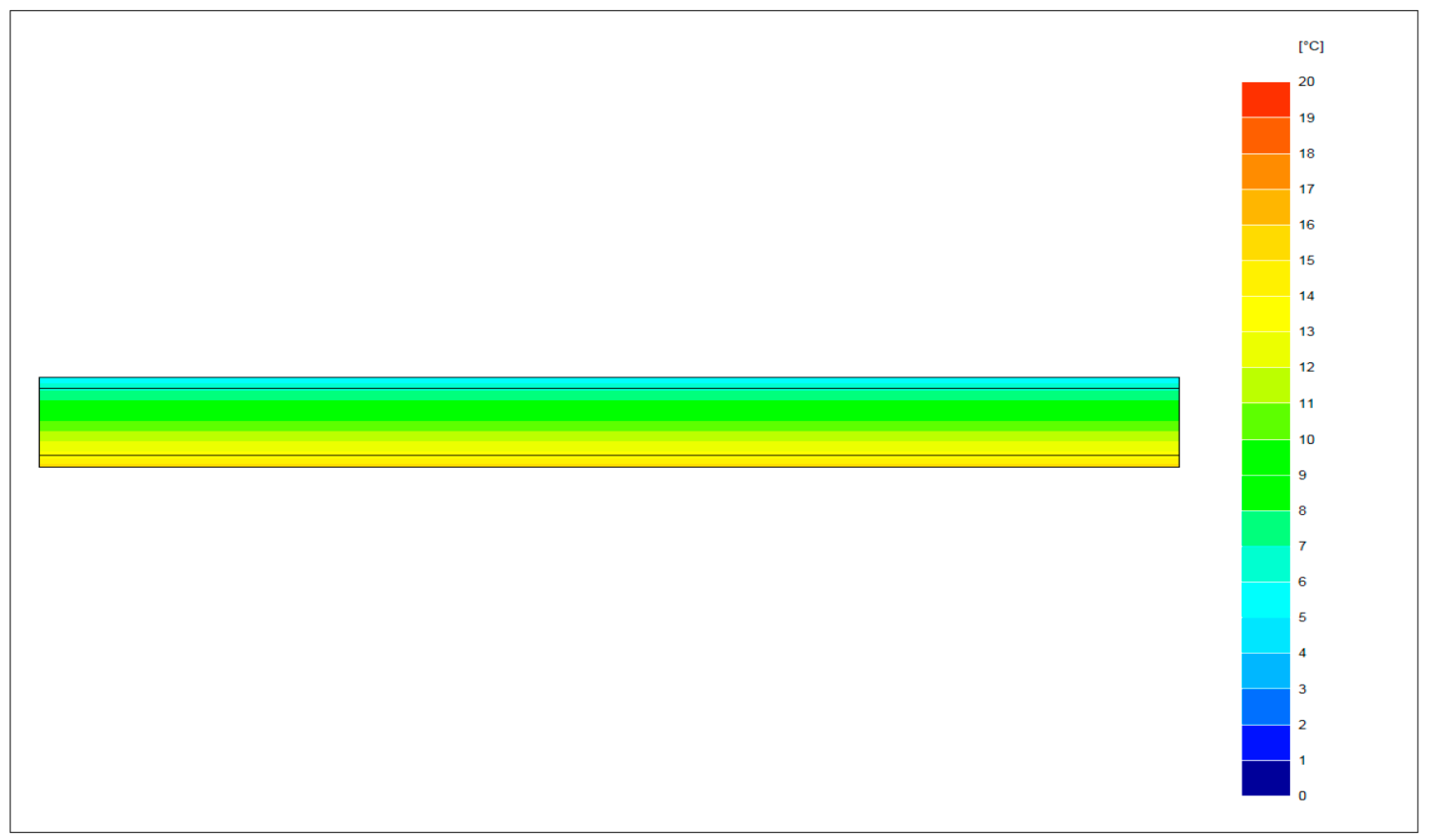
Internal Boundary Conditions
Operative temperature 20 °C
Overall internal surface resistance10 W/(m2 K) as per ISO EN BS 6946
External boundary conditions (assumed light breeze)
Air temperature 18.7 °C
Sky temperature −21 °C
Convective surface resistance 5 W/(m2 K)
Surface conditions
Surface emissivity 0.95
Surface temperature 5.2 °C

