Abstract
The synthetic aperture radar (SAR) image of moving targets will defocus due to the unknown motion parameters. For fast-maneuvering targets, the range cell migration (RCM), Doppler frequency migration and Doppler ambiguity are complex problems. As a result, focusing of fast-maneuvering targets is difficult. In this work, an efficient SAR refocusing algorithm is proposed for fast-maneuvering targets. The proposed algorithm mainly contains three steps. Firstly, the RCM is corrected using sequence reversing, matrix complex multiplication and an improved second-order RCM correction function. Secondly, a 1D scaled Fourier transform is introduced to estimate the remaining chirp rate. Thirdly, a matched filter based on the estimated chirp rate is proposed to focus the maneuvering target in the range–azimuth time domain. The proposed method is computationally efficient because it can be implemented by the fast Fourier transform (FFT), inverse FFT and non-uniform FFT. A new deramp function is proposed to further address the serious problem of Doppler ambiguity. A spurious peak recognition procedure is proposed on the basis of the cross-term analysis. Simulated and real data processing results demonstrate the validity of the proposed target focusing algorithm and spurious peak recognition procedure.
1. Introduction
Synthetic aperture radar (SAR) can image the scenes of interest during the day and night regardless of weather conditions, which attracts considerable attention worldwide [1,2,3,4,5,6,7,8,9,10]. SAR has been widely used in numerous remote sensing applications, such as marine observation, traffic monitoring and antiterrorism. The growing demand for surveillance of moving targets has made imaging these targets a major task for modern SAR systems [11,12,13,14,15]. Nevertheless, the unknown motion parameters between the SAR platform and the moving target result in range cell migration (RCM) and Doppler frequency migration (DFM) [16,17]. These factors lead to the defocused image of moving targets. Thus, the defocusing effects induced by the RCM and DFM should be effectively removed.
Several methods have been presented to remove the RCM with the SAR system. The Hough/Radon transforms [18,19] were utilised to search the trajectory and correct the RCM. However, they suffer from high computational complexity due to the searching of the trajectory. On this basis, the first-order keystone transform (FOKT) [20,21], second-order keystone transform (SOKT) [22,23] and Doppler keystone transform [24] were proposed to remove the corresponding RCM without knowing a priori knowledge of the moving target. Although these transforms avoid searching of the target trajectory, their performance is limited by the effects of DFM and Doppler ambiguity. Methods, such as FOKT-based methods [25,26], stationary phase-based methods [27,28], joint time–frequency analysis-based methods [17,29] and modified SOKT-based methods [30], were presented to deal with these issues. However, these methods ignore the acceleration motion and only consider the moving target with a low-order (i.e., second-order) phase model. The acceleration motion and third-order phase should be further considered for the fast-maneuvering target [16,31,32]. Thus, the aforementioned methods may be inappropriate.
The components of RCM and DFM become increasingly complex due to the acceleration motion and third-order phase. Different from the RCM and DFM for moving targets with a low-phase model, which only includes first-order RCM (FRCM), second-order RCM (SRCM) and linear DFM (LDFM), the third-order RCM (TRCM) and quadratic DFM (QDFM) should be included for fast-maneuvering targets. The first-order phase of the target signal induces the Doppler centre shift; then, the Doppler centre ambiguity emerges due to the limitation of pulse repetition frequency (PRF) for the SAR system [25,27]. The complex azimuth Doppler spectrum induced by Doppler centre shift and DFM may distribute into one, two or multiple PRF bands. When the azimuth Doppler spectrum occupies two or multiple PRF bands, the target spectrum split occurs, which induces the Doppler spectrum ambiguity. The TRCM, QDFM, Doppler centre blur and spectrum ambiguity lead to the difficulty in the focusing of fast-maneuvering targets.
The axis mapping-based coherently integrated cubic phase function (CICPF) method [31] was introduced in consideration of the acceleration motion and third-order phase. However, this method directly applies SOKT to remove the SRCM and ignores the complex Doppler spectrum ambiguity (i.e., Doppler spectrum spanning over two or multiple PRF bands). If the Doppler spectrum is not located entirely on one PRF band, then the target trajectory will split into multiple parts after performing this method. A SOKT-based generalised Hough-high-order ambiguity function (SOKT-GHHAF) method [32] was proposed to focus the maneuvering targets for dealing with the aforementioned issue. This method uses the operation of Doppler centre shifting by PRF/2 to eliminate the effect of Doppler spectrum split. However, if the target spectrum bandwidth is larger than PRF/2, then the operation of Doppler centre shifting by PRF/2 will be invalid, and the effect of Doppler spectrum split will still persist [25]. The parameter searching-based methods [16,33] were introduced without the effect of Doppler spectrum ambiguity. Although these algorithms are effective, they suffer from large computational complexity induced by a brute-force parameter searching procedure.
We present a new computationally efficient algorithm for refocusing of ground fast-maneuvering targets on the basis of the previous works. In this algorithm, the RCM is corrected using sequence reversing, matrix complex multiplication and an improved SRCM correction function in the range frequency and azimuth slow time domain. The Doppler centre shift is removed simultaneously. Then, a 1D scaled Fourier transform (SCFT) with the constant factor is used to estimate the chirp rate of the target signal. Thereafter, a matched filter based on the estimated chirp rate is presented to focus the moving target in the range–azimuth time domain. In addition, a new deramp function with the constant factor is proposed to further deal with the Doppler spectrum ambiguity. Then, the operation of combining the new deramp function and SOKT is introduced to address the mismatch of the improved SRCM correction function. The cross-term interference for multiple targets is analysed, and a spurious peak recognition procedure is proposed. The simulated and real data processing results verify the proposed target focusing algorithm and spurious peak recognition procedure.
The main contributions of this work are listed as follows: (1) the proposed algorithm can achieve a well-focused result in the range–azimuth time domain because the acceleration motion and third-order phase of the fast-maneuvering target are considered; (2) the presented algorithm has low computational complexity given that it can be implemented by the fast Fourier transform (FFT), inverse FFT (IFFT) and non-uniform FFT (NUFFT); (3) two constant factors, namely, and , are introduced to expand the applicability of the proposed algorithm; (4) a new deramp function is introduced to further deal with the complex Doppler ambiguity; and (5) a spurious peak recognition procedure is presented to address the cross-term interference.
The rest of the paper is organised as follows: Section 2 provides the signal model and characteristics. Section 3 describes the proposed algorithm. Section 4 gives specific analysis related to the proposed algorithm. Section 5 presents the simulated and real data processing results. Section 6 gives the discussion of the proposed algorithm. Section 7 provides the final conclusions.
2. Signal Model and Characteristics
2.1. Signal Model
The motion geometry between the SAR platform under the side-looking strip-map mode and the ground maneuvering target on a slant-rang plane is shown in Figure 1. During the synthetic time , the SAR platform flies with constant velocity . The maneuvering target with cross-track velocity , cross-track acceleration , along-track velocity and along-track acceleration moves from point A to point B. and denotes the nearest and instantaneous slant ranges between the SAR platform and the maneuvering target. represents the azimuth slow time.
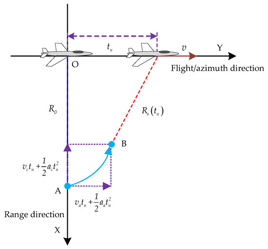
Figure 1.
Motion geometry between the synthetic aperture radar platform and the ground maneuvering target on a slant-rang plane.
In accordance with the motion geometry described in Figure 1, is expressed as
The instantaneous slant range can be expanded on the basis of the Taylor series expansion. Considering the accuracy of the range model, a third-order range model is used as follows [16,31,32,33]:
We suppose that the radar transmits the linear frequency modulation (LFM) signal with the form as follows [20]:
where indicates the range time, is the rectangle window function, denotes the pulse length, is the chirp rate of the transmitted signal and represents the carrier frequency. The received baseband signal is written as
where is the backscattering coefficient of the moving target, denotes the speed of electromagnetic wave, is the azimuth window function and is the wavelength of the transmitted signal.
By substituting Equations (2) into (4) and performing the range compression [20,22], the received signal omitting the envelope in the range frequency and azimuth time domain yields
where denotes the range frequency variable and is the bandwidth of the transmitted signal.
After the range IFFT is applied to Equation (5), the received signal in the range and azimuth slow time domain is expressed as
where denotes the sinc function.
2.2. Signal Characteristics
In accordance with Equation (5), the range frequency variable is coupled with the azimuth slow time variable . Not only the coupling effects caused by the low-order terms, namely, the - and -term, but also those induced by the high-order one, namely, the -term, exist. Therefore, the range position and Doppler frequency of the moving target change with the azimuth slow time.
As described in the sinc function term of Equation (6), the -term induces FRCM, the -term causes SRCM and the -term leads to TRCM in the range dimension. According to the last exponential term of Equation (6), the -term, -term and -term result in Doppler centre shift, LDFM and QDFM, respectively, in the Doppler frequency dimension. The RCM and DFM are severe for fast-maneuvering targets. This condition makes the trajectory span over multiple ranges and Doppler frequency cells. Thus, the complex RCM and DFM should be effectively removed to focus the moving target.
The target azimuth Doppler spectrum distribution must be further studied to obtain a well-focused result [34]. The Doppler centre shift of the fast-maneuvering target is larger than PRF/2, and the target shows Doppler centre blur. In the 2D spectrum dimension, the potential azimuth spectrum distributions caused by Doppler centre shift and DFM consist of the following cases. When , where denotes the azimuth spectrum bandwidth of the target signal, two azimuth spectrum distributions are introduced: case I: the azimuth spectrum is located entirely on one PRF band, as shown in Figure 2a, where represents the Doppler centre shift in the figure; case II: the azimuth spectrum spans over two PRF bands, as shown in Figure 2b. When , two other azimuth spectrum distributions are obtained: case III: the azimuth spectrum still occupies one PRF band, as displayed in Figure 2c; case IV: the azimuth spectrum also distributes into two PRF bands, as shown in Figure 2d. When , as shown in Figure 2e, the azimuth spectrum distributes into several PRF bands. When the azimuth spectrum does not entirely occupy one PRF band, namely, cases II, IV and V, the target spectrum split will occur; this phenomenon induces the azimuth Doppler spectrum ambiguity [34,35].
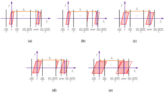
Figure 2.
Potential azimuth Doppler spectrum distributions: (a) case I: , spectrum entirely in one pulse repetition frequency (PRF) band; (b) case II: , spectrum spanning two PRF bands; (c) case III: , spectrum entirely in one PRF band; (d) case IV: , spectrum spanning two PRF bands; (e) case V: , spectrum spanning several PRF bands.
In summary, the complex RCM and DFM lead to severe integration loss and defocusing of the target image. In the existing methods, the Doppler ambiguity number searching [25,34] and Doppler centre shifting by PRF/2 operations [26,27,32] were usually used to deal with the Doppler centre blur and spectrum ambiguity, respectively. However, the Doppler ambiguity number searching operation increases the computational complexity. If the spectrum distribution belongs to case IV or V, then the Doppler centre shifting by PRF/2 operation will be invalid. Accordingly, the moving targets become difficult to be focused in the presence of complex Doppler ambiguity by applying transitional FOKT or SOKT-based [20,21,22,23,24,25,26,31,32] and stationary phase-based [27,28] methods. We present a new algorithm for refocusing of fast-maneuvering targets to deal with aforementioned problems.
3. Proposed Algorithm Description
The RCM, DFM, Doppler centre shift and Doppler ambiguity are the key issues for refocusing of fast-maneuvering targets according to the target signal properties described in the previous section. Therefore, a new fast algorithm is presented in this section.
3.1. RCM, Doppler Centre Shift and QDFM Compensation
In accordance with Equation (5), the discrete form of omitting the azimuth window function is expressed as
where denotes the discrete range frequency number index related to continuous range frequency , is assumed to be an even integer, denotes the range frequency sampling interval, represents the discrete slow time number index related to continuous slow time , is assumed to be an even integer and indicates the pulse repetition interval.
Given the symmetrical property of the discrete slow time sequence, a new signal after reversing the discrete slow time sequence for each range frequency yields [36,37]
where “” denotes the sequence reversing operation. As shown in Equations (7) and (8), the effects of -term and -term can be removed by multiplying Equation (7) by Equation (8). Thus, the corresponding result yields
As described in Equation (9), the FRCM, TRCM and QDFM are effectively compensated. In the meantime, the Doppler centre blur and spectrum distributions belonging to cases II and IV are avoided given that the Doppler centre shift is effectively removed. Nevertheless, the effect induced by -term still exists. Thus, the SRCM and FDFM should be effectively eliminated.
As verified in [16,33,38,39], the SRCM of the common metre-level range resolution SAR system depends on the SAR platform velocity given that the target along-track velocity and cross-track acceleration are considerably smaller than the velocity of SAR platform. Therefore, the SRCM can be removed by constructing the correction function on the basis of the SAR platform velocity as long as the residual SRCM correction error is smaller than one range resolution bin. In accordance with Equation (9), an improved SRCM correction function is constructed as follows:
The SRCM correction error by applying the correction function in Equation (10) is obtained as
We suppose that a maneuvering target, which is denoted by Target A, is considered. The target parameters are , , and . The main radar parameters are , , , , and . The SRCM correction error is calculated as 0.486 m, which is smaller than one range resolution bin. Example A without noise is also presented. Figure 3a shows the target trajectory after range compression. The target suffers from severe RCM effect. As illustrated in Figure 3b, only the SRCM remains after FRCM and TRCM correction. Figure 3c exhibits the result of SRCM compensation by using the correction function in Equation (10). The SRCM is effectively removed, and the trajectory of the moving target is located on the same range bin. The residual SRCM correction error by using the SAR platform velocity can be ignored and the correction function in Equation (10) is considered effective for the common metre-level range resolution SAR system.
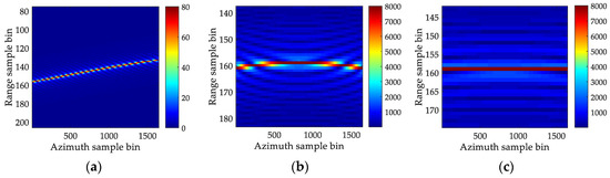
Figure 3.
Results of Example A: (a) trajectory after range compression; (b) trajectory after first-order range cell migration and third-order range cell migration correction; (c) result of second-order range cell migration correction by using the correction function in Equation (10).
After multiplying Equation (9) by Equation (10), we have
After the range IFFT is applied to Equation (12), the continuous time expression is obtained as
According to Equation (13), the moving target is focused in the same range bin, and the target signal along azimuth slow time dimension can be modelled as a second-order phase signal (i.e., an LFM signal). The chirp rate (i.e., second-order phase coefficient) of the target signal in Equation (13) should be effectively estimated and compensated to focus the moving target.
3.2. Estimation of Chirp Rate by 1D SCFT
Several typical methods, such as, discrete chirp-Fourier transform (DCFT) [34,40], fractional Fourier transform (FRFT) [29,41], Lv’s distribution (LVD) [26,42], and CICPF [17,31], have been proposed to estimate the chirp rate of the target signal in Equation (13). As for the parameter searching-based methods, DCFT and FRFT are computationally prohibitive due to the brute-force grid searching operation. Subsequently, the LVD and CICPF have been proposed without the searching process. However, these methods must transform the 1D LFM signal into a 2D parameter space to obtain the final estimation result. These methods still have a large computational burden due to the 2D data processing operation. Considering that the chirp rate of signal in Equation (13) has been doubled, the constant factor is introduced to expand the application scope. The corresponding 1D SCFT with constant factor yields
where , is the azimuth scaled frequency variable corresponding to and denotes the Dirac delta function. The selection criterion of constant factor is discussed in Appendix A.
In accordance with Equation (14), the chirp rate is estimated as follows:
where denotes the peak position in the azimuth scaled frequency domain.
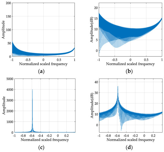
Example B without noise is provided to validate the constant factor . We consider a target that is denoted by Target B. The parameters of Target B are as follows: and . The radar parameters are the same as those of Example A. Figure 4a,b show the result using the 1D SCFT with the constant factor . The defocusing result is obtained in Figure 4a,b because the chirp rate of the signal for Target B exceeds the scope of parameter estimation. Figure 4c,d depict the result using the 1D SCFT with the constant factor . Given that the constant factor expands the parameter estimation scope, a clear peak appears in Figure 4c,d. Therefore, the results of Example B demonstrate the validity of the constant factor .
3.3. Azimuth Focusing by Matched Filter Based on Estimated Chirp Rate
The signal in Equation (9) is transformed into the range and azimuth frequency domain yields
By substituting Equation (15) into Equation (16), we have
In accordance with Equation (17), the matched filter based on the estimated chirp rate is constructed as follows:
After Equation (17) is multiplied by Equation (18) and 2D IFFT is performed, we have
where denotes the bandwidth of the signal in Equation (9).
As shown in Equation (19), the RCM, Doppler centre shift and DFM of the maneuvering target are effectively compensated. After 2D IFFT is performed, the moving target is refocused in the range–azimuth time domain; accordingly, the subsequent moving target processing operations are facilitated [22].
Figure 5 provides the flowchart of the presented algorithm. As shown in Figure 5, the proposed algorithm after range compression mainly includes three steps. The steps are summarised as follows:
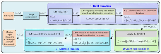
Figure 5.
Flowchart of the presented algorithm.
- (1)
- RCM correction
- (1.1)
- Apply the range FFT to the range compressed signal , and obtain .
- (1.2)
- Perform the sequence reversing operation to , and calculate Equation (9) to obtain .
- (1.3)
- Construct the SRCM correction function , and calculate Equation (12) to obtain .
- (2)
- Estimate the chirp rate by using the 1D SCFT, and obtain .
- (3)
- Azimuth focusing
- (3.1)
- Construct the azimuth match filter , and multiply Equation (16) by to obtain .
- (3.2)
- Perform 2D IFFT to , and obtain the final focused result ,
where step 1.1 is used to transform the range compressed signal into the range frequency domain, step 1.2 is applied to correct FRCM and TRCM, step 1.3 is performed to remove SRCM, step 3.1 is utilised to compensate LDFM and step 3.2 is used to obtain the final refocused result.
4. Analysis Related to the Proposed Algorithm
4.1. Analysis of the SRCM Correction Function Mismatch
Considering that the SRCM correction error may be larger than one range resolution cell in some high-range resolution SAR systems, the mismatch of SRCM correction function in Equation (10) will appear. As for this case, we can utilise the SOKT to correct the SRCM. However, the Doppler bandwidth of Equation (9) is easily larger than one PRF band because the chirp rate has been doubled after the previous processing steps. Then, the target trajectory will split into multiple parts after directly using SOKT due to the Doppler spectrum ambiguity (i.e., the azimuth spectrum distribution belonging to case V). Therefore, the Doppler bandwidth of Equation (9) should be effectively compressed. In [25,34], the deramp functions are constructed to compress the azimuth spectrum. However, these deramp functions ignore the effects of the target unknown motion parameters; this condition leads to the performance degradation, especially for fast-maneuvering targets. In accordance with Equation (9), the Doppler bandwidth is expressed as follows:
A new deramp function with constant factor is created to compress the Doppler bandwidth as follows:
By multiplying Equation (9) by Equation (21), we have
In accordance with Equation (22), the residual Doppler bandwidth is written as
As shown in Equation (23), the main part of Doppler bandwidth is removed. The Doppler bandwidth is extremely compressed. An appropriate constant factor is chosen to make the remaining Doppler bandwidth less than one PRF. The value of constant factor depends on the Doppler bandwidth of signal in Equation (9). If , then the constant factor will be chosen as . After the pre-processing step in Equation (23), the SOKT (i.e., [22,23]) can be applied to remove the SRCM. As a result, we have
As exhibited in Equation (24), the coupling influence between the -term and range frequency variable is eliminated. The SRCM is accurately removed after the SOKT is used, which is beneficial to the subsequent refocusing processing of a moving target. The target trajectory split is avoided because the Doppler bandwidth is effectively compressed. The Doppler spectrum ambiguity is further eliminated by performing a new deramp function. In the meantime, the constant factor is introduced to change the Doppler bandwidth of the deramp function. Thus, the new deramp function has a wide applicability.
Some noise-free simulation results are presented to validate the above-mentioned processing step. The range bandwidth of the simulated radar is set to 300 MHz. Other main radar parameters are the same as those of Example A. In Example C, a target, which is denoted by Target C, is considered. The parameters of the target are as follows: , , and .
Figure 6 shows the result of Example C. An evident SRCM appears in Figure 6a. Figure 6b displays the result of SRCM compensation by using the correction function in Equation (10). The residual SRCM correction error cannot be ignored because it is larger than one range bin. Therefore, the mismatch of the SRCM correction function in Equation (10) appears. The Doppler spectrum distribution of Target C after FRCM and TRCM correction is presented in Figure 6c. The Doppler spectrum bandwidth is larger than one PRF and the Doppler spectrum occupies several PRF bands because the chirp rate has been doubled after previous processing steps. The trajectory splits into several parts after directly performing the SOKT, as shown in Figure 6d. Figure 6e illustrates the result of applying the new deramp function with constant factor . The target Doppler spectrum bandwidth is extremely compressed, and the target Doppler spectrum is smaller than one PRF band. Figure 6f exhibits the result of performing the deramp and SOKT operations. Given that the target spectrum is located on one PRF band, the trajectory is focused in the same range bin after applying SOKT. Thus, the simulation results verify the new deramp function and SOKT operations.
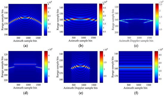
Figure 6.
Results of Example C: (a) trajectory of Target C after FRCM and TRCM compensation; (b) result using the correction function in (10); (c) trajectory of Target C in the range and Doppler domain; (d) result by directly using the second-order keystone transform (SOKT); (e) result after applying the new deramp function in Equation (21); (f) result after performing new deramp function and SOKT.
4.2. Analysis of Multiple Target Focusing
In the previous section, the case of one moving target is considered. However, multiple targets may be present in the observation scene. In the case of multiple targets, the effect of cross term induced by nonlinear operation in Equation (9) should be discussed. We assume that the number of targets is D. Then, the range compressed signal in Equation (5) is expressed as
where is the nearest slant range of the ith target. , and represent the first-, second- and third-order phases of the ith target, respectively.
The target signal after RCM correction (RCMC) is written as follows:
where
and denotes the cross terms of the signal in Equation (26). Given that the proposed method contains the nonlinear operation, the signal in Equation (26) includes auto and cross terms. According to Equations (26) and (27), the RCMs of auto terms are effectively eliminated, and only the second-order phase remains. Considering that the 1D SCFT is a linear transform, the second-order phases of the auto terms can be effectively estimated by the 1D SCFT. The matched filtering operation in Equation (18) is also a linear processing step. Thus, the auto terms can be refocused using the corresponding matched filters. With regard to the cross terms, and generally hold because , , and usually differ. Not only the second-order phases, but also the first- and third-order phases of the cross terms remain. Therefore, the RCMs of the cross terms still exist, and the energy of cross terms spreads along the range dimension. The cross terms are typically defocused in the 1D SCFT domain. In summary, the cross terms may not affect the refocusing of auto terms in this case.
However, moving targets may have the same first- and third-order phases, namely, and , respectively, in a particular case. Therefore, the signal in Equation (26) is simplified and transformed into range and azimuth slow time domain as follows:
In accordance with Equation (28), the RCMs of auto and cross terms are all removed. The auto terms are focused at the positions of , and the cross terms are focused at the positions of . Then, the 1D SCFT is performed to the auto and cross terms. Accordingly, we have
According to Equations (29) and (30), the peak positions of the auto and cross terms in the 1D SCFT domain are and , respectively.
The peaks of the cross terms may not affect the determination of the auto term peaks according to the previous analysis, but they may lead to spurious peaks. As shown in Equations (29) and (30), the peak positions of the auto terms, namely, and , are symmetric with respect to the peak positions of the cross terms, that is, , in the range time and 1D SCFT domain.
In summary, Figure 7 shows the symmetric characteristics between the auto and the cross terms. As shown in Figure 7a, trajectories of auto terms A and B are represented by a straight purple line, and that of the corresponding cross term C is denoted by a straight red line. After RCMC, auto terms A and B and cross term C are focused in the range time domain. The positions of the auto terms in the range time domain, namely, and , are symmetric with respect to the position of corresponding cross term . Figure 7b–d depict the 1D SCFT result of auto term A, cross term C and auto term B, respectively. The positions of the auto terms in the 1D SCFT frequency domain, namely, and , are symmetric with respect to the position of the cross term, that is, . Thus, the symmetric properties of the auto and cross terms in the range time and 1D SCFT domain can be used to preliminarily identify the potential spurious peak induced by the cross term.
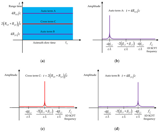
Figure 7.
Schematic of the symmetric characteristics between the auto and cross terms: (a) result of the auto and cross terms after range cell migration correction (RCMC); (b) 1D scaled Fourier transform (SCFT) result of auto term A; (c) 1D SCFT result of cross term C; (d) 1D SCFT result of auto term B.
A spurious peak recognition procedure based on the 1D SCFT is presented to confirm the potential spurious peak caused by the cross term. Firstly, a recognition function is proposed in the range frequency and azimuth slow time domain as follows:
After the SOKT is applied to the signal in Equation (31), we have
where
The signal in Equation (32) contains auto terms and cross terms. After the range IFFT is performed, we have
where represents the result of transforming the cross terms in Equation (33) into the range and azimuth slow time domain. If the first- and third-order phases do not satisfy and , as shown in Equation (33), then not only the second-order phases, but also the first and third-order phases of cross terms remain for the recognition function. Therefore, the RCMs and DFMs of the cross terms exist, and the energy of cross terms is still defocusing. The first-, second- and third-order phases of the auto terms are removed. The auto terms are focused at the position of in the range time domain.
As for the special case, namely, and , Equation (32) is rewritten as follows after the range IFFT is applied:
According to Equation (35), the auto terms of the recognition function in Equation (35) are focused at and the cross terms of the recognition function in Equation (35) are focused at and in the range domain. Then, the 1D SCFT is applied to the cross terms of the recognition function in Equation (35). As a result, we have
As shown in Equation (36), the peak positions of cross terms are and , respectively, in the 1D SCFT domain.
Therefore, the peak positions of the cross terms of the recognition function in Equation (35), namely, and , are symmetric with respect to the position of .
In summary, Figure 8 shows that, if the peak is the spurious peak, then the recognition function will have evident symmetrical peaks with the same amplitudes at positions of and , which are symmetric with respect to the position of . Otherwise, Figure 9 depicts that, if the peak is the target peak, then the evident symmetrical peaks at positions of and are absent in the output result of the recognition function.
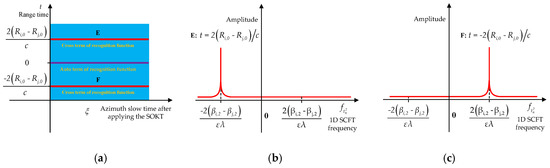
Figure 8.
Result of spurious peak recognition function for spurious peak: (a) RCMC result; (b) 1D SCFT result for signal in ; (c) 1D SCFT result for signal in .
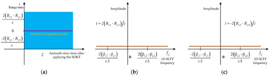
Figure 9.
Result of spurious peak recognition function for target peak: (a) RCMC result; (b) 1D SCFT result for signal in ; (c) 1D SCFT result for signal in .
The identification procedure of the potential spurious peak is summarised as follows:
Step 1) Extract all peak positions, which are denoted by , where is the number of peaks.
Step 2) Determine whether and , , , , is satisfied; if so, then the peak at position of may be the spurious peak of the cross term. Apply the recognition function (i.e., Steps 3–5) to identify the potential spurious peak; if not, then all peaks are the target peaks.
Step 3) Calculate Equation (31), and obtain .
Step 4) Perform the SOKT and range IFFT to , and obtain .
Step 5) Apply azimuth 1D SCTF to and . If evident symmetrical peaks with the same amplitudes described in Figure 8 are present, then the peak at mentioned in Step 2 will be a spurious peak. Otherwise, the peak at is the target peak.
The flowchart of potential spurious peak recognition procedure is given in Figure 10.
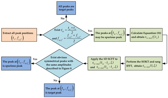
Figure 10.
Flowchart of the potential spurious peak identification procedure.
Two examples are provided to validate the analysis of multiple target focusing and spurious peak recognition procedure. The radar parameters are the same as those of Example A. The signal-to-noise (SNR) is 7 dB. In Example D, we consider three targets with different motion parameters, and that are represented by Targets D, E and F. The phase parameters of these target signals are
Figure 11 displays the processing results of Example D. Figure 11a depicts the RCMC result. The background noise is removed from the obtained result to show the target trajectories clearly. Three straight trajectories related to Targets D, E and F appear because the RCM is effectively corrected. However, the cross terms are still defocused due to the serious effect of the RCM, thereby helping in suppressing the interference of the cross term. Figure 11b–d exhibit the 1D SCFT results for Targets D, E and F in the 147th, 177th and 207th range sample bins, respectively. Evident peaks with respect to Targets D, E and F appear in the corresponding figure. Figure 11e,f illustrate the 1D SCFT results of data in the 157th and 187th range sample bins, respectively, to indicate the defocusing of cross terms without loss of generality. The evident peaks are absent in the processing results. The cross terms still suffer from the effect of defocusing induced by the residual first- and third-order phase errors. The positions of peaks in Figure 11b–d satisfy the symmetric properties described in Figure 7. The potential spurious peak recognition procedure is utilised to identify whether the peak in Figure 11c is a spurious peak. Figure 12a,b depict the corresponding recognition result. Considering that clear peaks, which satisfy the symmetric feature shown in Figure 8, do not emerge in the 30th and −30th range time sample bins of the recognition function, the peak in Figure 11c is determined as the target peak.
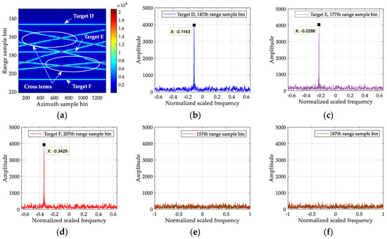
Figure 11.
Results of Example D: (a) result after RCMC; (b) 1D SCFT result for Target D in the 147th range sample bin of Figure 11a; (c) 1D SCFT result for Target E in the 177th range sample bin of Figure 11a; (d) 1D SCFT result for Target F in the 207th range sample bin of Figure 11a; (e) 1D SCFT result of data in the 157th range sample bin of Figure 11a; (f) 1D SCFT result of data in the 187th range sample bin of Figure 11a.
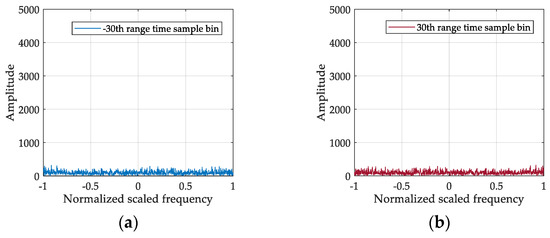
Figure 12.
Potential spurious peak recognition results of Example D: (a) 1D SCFT result of the −30th range time sample bin of the recognition function; (b) 1D SCFT result of the 30th range time sample bin of the recognition function.
In Example E, we consider two targets that are denoted by Targets G and H. The phase parameters of these target signals are
Figure 13 shows the obtained results of Example E. The RCMC result without noise is exhibited in Figure 13a to display the target trajectories clearly. Three straight trajectories are observed in Figure 13a because the first- and third-order phases of Target G equal those of Target H. Figure 13b–d illustrate the 1D SCFT result of the data in the 147th, 177th, and 207th range sample bins, respectively. Considering that peak positions in Figure 13b–d satisfy the symmetric characteristics described in Figure 7, the peak in Figure 13c may be a spurious peak. Figure 14 depicts the potential spurious peak recognition results. Given that evident symmetric peaks with the same amplitudes appear in the 30th and −30th range time sample bins of the recognition function, as shown in Figure 14a,b, the peak in Figure 13c is confirmed as the spurious peak.
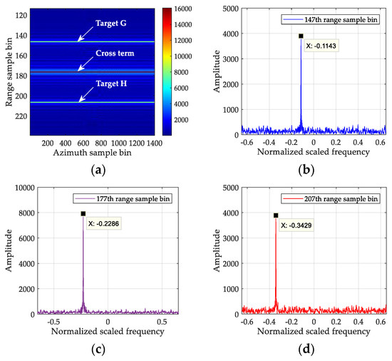
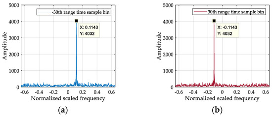
Figure 14.
Potential spurious peak recognition results of Example E: (a) 1D SCFT result of the −30th range time sample bin of the recognition function; (b) 1D SCFT result of the 30th range time sample bin of the recognition function.
5. Experimental Results
In this section, several simulation experimental results in the presence of Gaussian background and real data processing results are analysed to verify the proposed method.
5.1. Simulation Experimental Result Analysis
The simulation radar parameters are listed in Table 1. Two maneuvering targets, which are denoted by T1 and T2, are considered. The motion parameters of the two targets are summarised in Table 2. The SNR after range compression is 8 dB. T1 is a Doppler spectrum ambiguity target, and its azimuth Doppler spectrum bandwidth is larger than PRF/2. The azimuth Doppler spectrum of T1 distributes into two PRF bands. The Doppler ambiguity number of T2 is −1, and its azimuth Doppler spectrum is still located on one PRF band. The constant factor is set to following the constant factor selection strategy in Appendix A. The FOKT-based [25], stationary phase-based [28] and SOKT-GHHAF methods [32] are used for comparison.

Table 1.
Basic simulation radar parameters.
Table 2.
Simulation parameters for two targets.
Figure 15a depicts the result of range compression. Two curved trajectories are observed in the figure. Target energy also distributes into several range sample bins, thereby leading to severe RCM. The result by directly applying azimuth FFT is illustrated in Figure 15b. Notably, the energy of targets also spreads along the azimuth Doppler dimension, which induces serious DFM. The RCM and DFM result in severe defocusing effects. In addition, the azimuth Doppler spectrum of T1 spans over two PRF bands. The azimuth Doppler spectrum of T2 occupies one PRF. Figure 15c shows the result after RCMC, and the background is removed to indicate the trajectories of two targets clearly. The RCM is effectively eliminated, and the trajectory split is avoided. The energy of the target is focused in the corresponding range bin. In the meantime, the RCMs of cross terms remain, and cross terms still suffer from the effect of defocusing, thereby helping in suppressing the cross terms. Figure 15d exhibits the 1D SCFT result of T1. An evident peak with respect to T1 appears in Figure 15d. From the peak position, a well-focused result is obtained in the range–azimuth time domain by using the corresponding matched filter, as shown in Figure 15e–h. For the same reason, T2 is also accumulated as a peak in Figure 15i. With the peak position, T2 is well focused in the range–azimuth time domain by the matched filtering, as exhibited in Figure 15j–m.
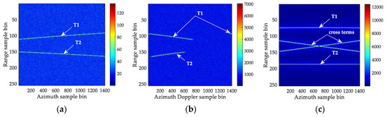
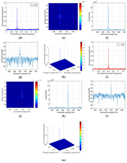
Figure 15.
Results of simulation experiment: (a) range compression result; (b) azimuth Doppler spectrum distributions of two targets; (c) RCMC result; (d) 1D SCFT result of T1; (e) focusing result of T1 by using the proposed method; (f) profile for focusing result of T1; (g) dB version of amplitude for Figure 15f; (h) stereogram of Figure 15e; (i) 1D SCFT result of T2; (j) focusing result of T2 by performing the proposed method; (k) profile for focusing result of T2; (l) dB version of amplitude for Figure 15k; (m) stereogram of Figure 15j.
Figure 16a,b plot the SRCM correction result using the SOKT-GHHAF method before and after Doppler centre shifting by PRF/2 operation. The background is removed from the result to illustrate the target trajectory clearly. As presented in Figure 16a, the trajectory of T1 splits into two parts due to the azimuth Doppler spectrum of T1 spanning over two PRF bands. Given that the Doppler spectrum bandwidth is larger than PRF/2, the operation of Doppler centre shifting by PRF/2 in SOKT-GHHAF method is invalid. Figure 16b exhibits that the trajectory still splits into two parts, and this condition affects the performance of RCMC and induces the coherent integration loss. Figure 16c–e show the focusing result of T1 by applying the FOKT-based method. A defocused result appears in Figure 16c–e because the along-track velocity and acceleration motions are ignored. As presented in Figure 16f–h, the focusing performance of the stationary phase-based method deteriorates significantly given that the third-order phase is neglected.
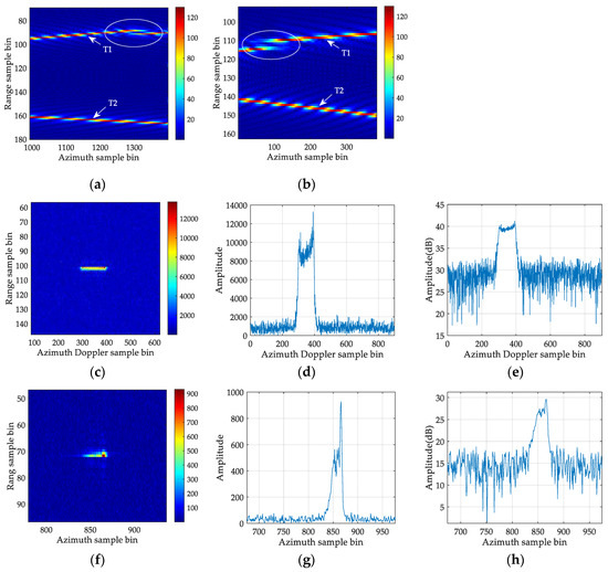
Figure 16.
Processing results of compared methods for T1: (a) SRCM compensation result using second-order keystone transform-based generalised Hough-high-order ambiguity function (SOKT-GHHAF) method before Doppler centre shifting by PRF/2; (b) SRCM correction result using SOKT-GHHAF method after Doppler centre shifting by PRF/2; (c) focusing result by performing the first-order keystone transform-based method; (d) profile for focusing result of FOKT-based method; (e) dB version of amplitude for Figure 16d; (f) focusing result by applying the stationary phase-based method; (g) profile for focusing result of the stationary phase-based method; (h) dB version of amplitude for Figure 16f.
In summary, the result of simulation experiment validates that the proposed method can effectively compensate the RCM and DFM of the maneuvering target, and a well-focused result can be achieved regardless of Doppler ambiguity including Doppler centre blur and spectrum ambiguity. The performance of presented method is better than that of the FOKT-based and stationary phase-based methods. This result is attributed to the fact that the proposed method considers the along-track velocity and acceleration motions and can deal with the high-order RCM and DFM induced by the third-order phase. The proposed method is also more robust to Doppler ambiguity than the SOKT-GHHAF method because it can effectively solve the problems of Doppler centre shift and Doppler spectrum broadening.
5.2. Real Data Processing Result Analysis
In this section, two parts of RADARSAT-1 Vancouver scene data [1,26] are utilised to validate the presented algorithm. These real radar data are recorded by a C-band space-borne SAR system. The main radar system parameters are summarised in Table 3. The detailed parameters of these real data are given by [1,26]. The azimuth pulse number of selected data is 1500.
Table 3.
Main radar parameters for RADARSAR-1.
5.2.1. Processing Result of a Single Target
Figure 17a shows the image of the selected scene, where the interested target is highlighted in the figure. Figure 17b depicts the trajectory for the target of interest after range compression. The trajectory distributes into multiple range sample bins due to the serious RCM, which indicates the typical defocusing. Figure 17c illustrates the result of RCMC in the range–Doppler domain. The target energy is focused in the same range bin after RCMC, but the effect of DFM still remains. As shown in Figure 17d, an evident peak appears in the 1D SCFT domain. According to the peak position in Figure 17d, the target can be focused by using the proposed method, as exhibited in Figure 17e. Therefore, the above-mentioned real data processing results demonstrate the effectiveness of the presented method.
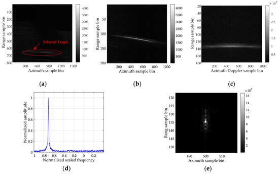
Figure 17.
Real data processing results of a single target: (a) image of the selected scene; (b) trajectory of interested target after range compression; (c) result after RCMC; (d) 1D SCFT result; (e) focusing result for a single target of interest.
5.2.2. Processing Result of Two Targets
Figure 18a displays the image of the selected scene, where the two targets of interest, which are denoted by Target 1 and Target 2, are marked in the figure. Figure 18b shows the trajectories of Target 1 and Target 2 after range compression. The profile along the 420th azimuth sample bin of Figure 18b is depicted in Figure 18c,d. Two trajectories span over several range sample bins due to the serious RCM. Figure 18e depicts the result of RCMC in the range–Doppler domain. The profile along the 420th azimuth Doppler sample bin of Figure 18e is shown in Figure 18f,g. The RCM is effectively removed, but the DFM still exists. The trajectory in the middle of trajectories for Target 1 and Target 2 is a potential cross term according to the analysis in Section 4.2. Figure 18h–j illustrate 1D SCFT results of data in the 69th range sample bin (Target1), 79th range sample bin (cross term) and 89th range sample bin (Target2), respectively. Given that the peak positions in Figure 18h–j satisfy the symmetric features described in Figure 7, the peak shown in Figure 18i is preliminarily identified as a potential spurious peak. The spurious peak recognition results are shown in Figure 19a,b. The peak illustrated in Figure 18i is confirmed as the spurious peak because the symmetric peaks with the same amplitudes appear in 10th and −10th range time sample bins of the recognition function. The cross term is removed, and the focused results of Target 1 and Target 2 are depicted in Figure 19c,d, respectively. These real data processing results verify that the proposed method can be used to focus multiple targets and validate the proposed spurious peak recognition procedure.
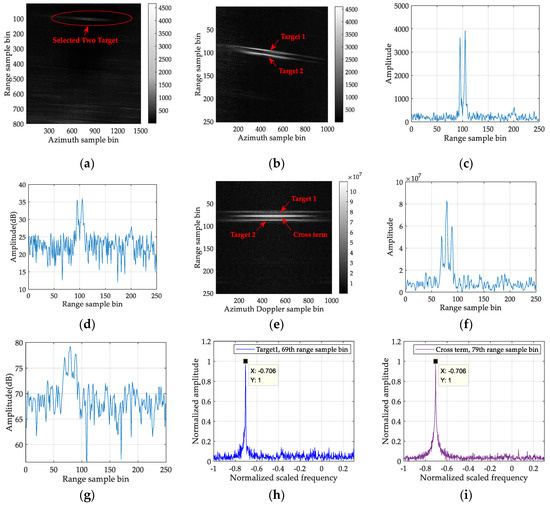
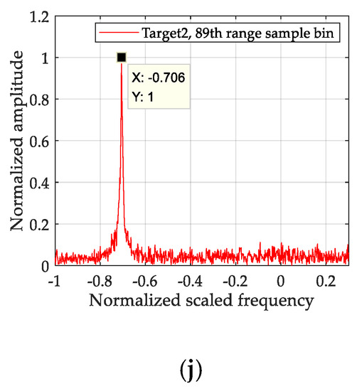
Figure 18.
RCMC and 1D SCFT results: (a) image of the selected scene; (b) range compression result for two targets of interest; (c) profile along the 420th azimuth sample bin of Figure 18b; (d) dB version of amplitude for Figure 18c; (e) result after RCMC; (f) profile along the 420th azimuth Doppler sample bin of Figure 18e; (g) dB version of amplitude for Figure 18f; (h) 1D SCFT result of the 69th range sample bin (Target 1); (i) 1D SCFT result of the 79th range sample bin (cross term); (j) 1D SCFT result of the 89th range sample bin (Target 2).
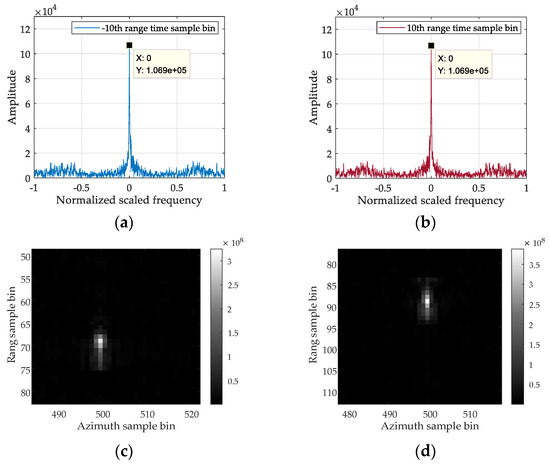
Figure 19.
Potential spurious peak recognition and final focusing results: (a) 1D SCFT result for the −10th range time sample bin of the recognition function; (b) 1D SCFT result for the 10th range time sample bin of the recognition function; (c) focusing result of Target 1; (d) focusing result of Target 2.
6. Discussion
6.1. Computational Complexity
In this section, we discuss the computational complexity of the proposed method, FOKT-based method [25], stationary phase-based method [28] and SOKT-GHHAF method [32]. Similar to [32], the number of complex multiplications is utilised to indicate the computational complexity. We suppose that represents the number of range bins and denotes the number of pulses. For convenience, we assume that the SRCM correction function in Equation (10) is effective. The computational burden of the proposed algorithm includes a range FFT operation, a point matrix complex multiplication, an SRCM correction operation, a 1D SCFT processing, an azimuth FFT operation, a matched filtering processing and a 2D IFFT operation. Notably, the 1D SCFT in Equation (14) can be easily implemented using the NUFFT of low computational burden. The detailed analysis of the NUFFT has been provided in [43,44]. The computational complexity of the NUFFT-based 1D SCFT is obtained using [43,44]. Thus, the total computational cost of the proposed method is denoted as . We assume that the searching times of and Doppler ambiguity number are represented by and , respectively. The computational cost of the SOKT-GHHAF method is denoted as [32]. The computational burden for stationary phase-based method is obtained using [28]. The computational complexity of the FOKT-based method is represented as [25].
In the case of the SRCM correction function mismatch, the SOKT operation should be added in the proposed method. The chirp-z-based SOKT is applied to compensate the SRCM. The computational cost of chirp-z-based SOKT is represented as [45]. The total computational burden is denoted as . In this case, the computational complexity of the proposed algorithm is slightly increased. However, the proposed method still has low computational complexity.
Table 4 exhibits the detailed computational costs of the above-mentioned algorithms. The table shows that proposed method1 denotes the computational complexity of the proposed method in the case of SRCM correction function matching, and proposed method2 represents the computational complexity of the proposed method in the case of SRCM correction function mismatch. In summary, the computational complexity of the proposed algorithm is lower than that of the SOKT-GHHAF, stationary phase-based and FOKT-based methods because it can be implemented using FFT, IFFT and NUFFT. The parameter searching procedure is avoided.
Table 4.
Comparison of computational complexities.
6.2. Some Remarks
Remark 1.
The different moving targets may have various scattering intensities for multiple target focusing. If the intensities of these targets are significantly different, then the target with higher intensity may submerge the target with a lower value; this condition affects the performance of the presented method. In this case, the CLEAN technique in [46,47] can be provided to remove the strong target effect. The strong and weak moving targets can be focused iteratively.
Remark 2.
The proposed method has a relatively high demand on the target input SNR/signal-to-clutter and noise ratio (SCNR) because its processing procedure contains a nonlinear operation. Therefore, the presented algorithm is suitable for the fast realisation for refocusing of fast-maneuvering targets in the case of relatively high SNR/SCNR. However, a slow and weak moving target may be drowned by the strong clutter background. In this case, the performance will degrade. At this time, many excellent clutter rejection methods, such as displaced phase centre antenna [48] and space-time adaptive processing [49,50], can be performed to reject the clutter. After clutter suppression, the proposed method can be used to refocus the moving target given that the target input SCNR is significantly increased. The effectiveness of clutter suppression in the moving target refocusing application has been validated in previous studies [16,17,25,27,29,32]. Interested readers may refer to [27,29] for a detailed analysis about clutter rejection in the moving target refocusing applications. The fast realisation for refocusing of moving targets with a low SNR/SCNR in strong or extremely heterogeneous background is still a challenging work and will be investigated in the future.
7. Conclusions
The unknown motion parameters of ground fast-maneuvering targets induce high-order RCM and DFM (i.e., CRCM and QDFM), which make the target energy seriously defocused. Fast-maneuvering targets easily exhibit complex Doppler ambiguity due to the limitation of PRF for SAR systems. These factors result in the difficulty in focusing of moving targets. In this work, a new computationally efficient algorithm is proposed to focus fast-maneuvering targets. The characteristics of the presented algorithm are summarised as follows: (1) the presented algorithm can effectively focus fast-maneuvering targets in the range–azimuth time domain because the acceleration and third-order phase are considered; (2) the proposed method is computationally efficient; (3) the proposed algorithm has a wide applicability because two constant factors and are introduced; (4) a new deramp function is proposed to further address the complex Doppler ambiguity including Doppler centre blur and spectrum ambiguity; (5) the cross-term interference for multiple target focusing is analysed, and a corresponding recognition procedure is proposed to identify the spurious peak. The effectiveness of the moving target refocusing algorithm and spurious peak recognition procedure has been confirmed by simulated and real data processing results. However, the proposed method introduces the nonlinear operation due to fast implementation for refocusing of fast-maneuvering targets; this condition weakens the performance in the case of low SNR/SCNR. This problem will be investigated in the future.
Author Contributions
Conceptualization, J.W. and L.Z.; Data curation, J.W. and Y.Z.; Formal analysis, J.W. and Z.C.; Funding acquisition, Y.Z. and L.Z.; Investigation, J.W. and H.Y.; Methodology, J.W. and Z.C.; Project administration, Y.Z. and L.Z.; Supervision, L.Z.; Validation, J.W., Y.Z. and Z.C.; writing—original draft, J.W.; writing—review and editing, Y.Z., L.Z., Z.C. and H.Y.
Funding
This research was funded by the National Natural Science Foundation of China, Grant Nos. 61871305, 61671361, and 61731023; and the APC was funded by the National Natural Science Foundation of China, Grant No. 61871305.
Acknowledgments
The authors would like to thank the anonymous reviewers for their valuable and useful comments and suggestions that helped improve the paper.
Conflicts of Interest
The authors declare no conflict of interest.
Appendix A
In this appendix, the selection criterion of the constant factor for 1D SCFT in our proposed method is discussed. In accordance with the peak in Equation (14), the equation is obtained as follows:
To ensure the constant factor matching, the following inequality should be satisfied:
where denotes the maximum value of .
We assume that the value scopes of target along-track velocity and cross-track acceleration are and . Accordingly, the following equation is obtained:
By substituting Equation (A3) into Equation (A2), we obtain:
In accordance with Equation (A4), the selection scope of constant factor is obtained as follows:
The constant factor should satisfy the inequality in Equation (A5). According to Equation (15), if a large constant factor is chosen, then the estimation error will be increased. Therefore, a smaller constant factor can be selected to improve estimation accuracy under the condition described in Equation (A5).
References
- Cumming, I.G.; Wong, F.H. Digital Processing of Synthetic Aperture Radar Data: Algorithm and Implementation; Artech House: Norwood, MA, USA, 2005. [Google Scholar]
- Moreira, A.; Iraola, P.P.; Younis, M.; Krieger, G.; Hajnsek, I.; Papathanassiou, K.P. A tutorial on synthetic aperture radar. IEEE Geosci. Remote Sens. Mag. 2013, 1, 6–43. [Google Scholar] [CrossRef]
- Gomba, G.; Parizzi, A.; Zan, F.D.; Eineder, M.; Bamler, R. Toward operational compensation of ionospheric effects in SAR interferograms: The split-spectrum method. IEEE Trans. Geosci. Remote Sens. 2016, 54, 1446–1461. [Google Scholar] [CrossRef]
- Bovenga, F.; Giacovazzo, V.M.; Refice, A.; Veneziani, N. Multichromatic analysis of InSAR data. IEEE Trans. Geosci. Remote Sens. 2013, 51, 4790–4799. [Google Scholar] [CrossRef]
- Bovenga, F.; Derauw, D.; Rana, F.M.; Barbier, C.; Refice, A.; Veneziani, N.; Vitulli, R. Multi-chromatic analysis of SAR images for coherent target detection. Remote Sens. 2014, 6, 8822–8843. [Google Scholar] [CrossRef]
- Filippo, B. COSMO-SkyMed staring spotlight SAR data for micro-motion and inclination angle estimation of ships by pixel tracking and convex optimization. Remote Sens. 2019, 11, 766. [Google Scholar] [CrossRef]
- Filippo, B.; Pia, A.; Danilo, O.; Carmine, C. Micro-motion estimation of maritime targets using pixel tracking in Cosmo-Skymed synthetic aperture radar data-an operative assessment. Remote Sens. 2019, 11, 1637. [Google Scholar]
- Iglesias, R.; Fabregas, X.; Aguasca, A.; Mallorqui, J.J.; López-Martínez, C.; Gili, J.A.; Corominas, J. Atmospheric phase screen compensation in ground-based SAR with a multiple-regression model over mountainous regions. IEEE Trans. Geosci. Remote Sens. 2014, 52, 2436–2449. [Google Scholar] [CrossRef]
- Qin, M.; Li, D.; Tang, X.; Cao, Z.; Li, W.; Xu, L. A fast high-resolution imaging algorithm for helicopter-borne rotating array SAR based on 2-D chirp-z transform. Remote Sens. 2019, 11, 1669. [Google Scholar] [CrossRef]
- Tang, S.; Zhang, L.; So, H.C. Focusing high-resolution highly-squinted airborne SAR data with maneuvers. Remote Sens. 2018, 10, 862. [Google Scholar] [CrossRef]
- Baumgartner, S.V.; Krieger, G. Simultaneous high-resolution wide-swath SAR imaging and ground moving target indication: Processing approaches and system concepts. IEEE J. Sel. Top. Appl. Earth Observ. Remote Sens. 2015, 8, 5015–5029. [Google Scholar] [CrossRef]
- Chen, Z.; Zhou, Y.; Zhang, L.; Wei, H.; Lin, C.; Liu, N.; Wan, J. General range model for multi-channel SAR/GMTI with curvilinear flight trajectory. Electron. Lett. 2019, 55, 111–112. [Google Scholar] [CrossRef]
- Huang, Y.; Liao, G.; Xu, J.; Li, J.; Yang, D. GMTI and parameter estimation for MIMO SAR system via fast interferometry RPCA method. IEEE Trans. Geosci. Remote Sens. 2018, 56, 1774–1787. [Google Scholar] [CrossRef]
- Rahmanizadeh, A.; Amini, J. An integrated method for simulation of synthetic aperture radar (SAR) raw data in moving target detection. Remote Sens. 2017, 9, 1009. [Google Scholar] [CrossRef]
- Chen, Z.; Zhang, L.; Zhou, Y.; Lin, C.; Tang, S.; Wan, J. A non-adaptive space-time clutter canceller for multi-channel synthetic aperture radar. IET Signal Process. 2019, 13, 472–479. [Google Scholar] [CrossRef]
- Huang, P.; Liao, G.; Yang, Z.; Ma, J. An approach for refocusing of ground fast-moving target and high-order motion parameter estimation using Radon-high-order time-chirp rate transform. Digit. Signal Process. 2016, 48, 333–348. [Google Scholar] [CrossRef]
- Li, D.; Zhan, C.; Ma, H.; Liu, H.; Su, J.; Liu, Q. An efficient SAR ground moving target refocusing method based on PPFFT and coherently integrated CPF. IEEE Access. 2019, 7, 114102–114115. [Google Scholar] [CrossRef]
- Oveis, A.H.; Sebt, M.A. Coherent method for ground-moving target indication and velocity estimation using Hough transform. IET Radar Sonar Navig. 2017, 11, 646–655. [Google Scholar] [CrossRef]
- Zeng, H.; Chen, J.; Wang, P.; Yang, W.; Liu, W. 2-D coherent integration processing and detecting of aircrafts using GNSS-based passive radar. Remote Sens. 2018, 10, 1164. [Google Scholar] [CrossRef]
- Perry, R.P.; DiPietro, R.C.; Fante, R.L. SAR imaging of moving targets. IEEE Trans. Aerosp. Electron. Syst. 1999, 35, 188–200. [Google Scholar] [CrossRef]
- Zhu, D.; Li, Y.; Zhu, Z. A Keystone transform without interpolation for SAR ground moving-target imaging. IEEE Geosci. Remote Sens. Lett. 2007, 4, 18–22. [Google Scholar] [CrossRef]
- Zhou, F.; Wu, R.; Xing, M. Approach for single channel SAR ground moving target imaging and motion parameter estimation. IET Radar Sonar Navig. 2007, 1, 59–66. [Google Scholar] [CrossRef]
- Kirkland, D. Imaging moving targets using the second-order keystone transform. IET Radar Sonar Navig. 2011, 5, 902–910. [Google Scholar] [CrossRef]
- Li, G.; Xia, X.G.; Peng, Y. Doppler keystone transform: An approach suitable for parallel implementation of SAR moving target imaging. IEEE Geosci. Remote Sens. Lett. 2008, 5, 573–577. [Google Scholar] [CrossRef]
- Sun, G.; Xing, M.; Xia, X.G.; Wu, Y.; Bao, Z. Robust ground moving-target imaging using deramp-keystone processing. IEEE Trans. Geosci. Remote Sens. 2013, 51, 966–982. [Google Scholar] [CrossRef]
- Tian, J.; Cui, W.; Xia, X.G.; Wu, S. Parameter estimation of ground moving targets based on SKT-DLVT processing. IEEE Trans. Comput. Imaging 2016, 2, 13–26. [Google Scholar] [CrossRef]
- Zhu, S.; Liao, G.; Qu, Y.; Zhou, Z.; Liu, X. Ground moving targets imaging algorithm for synthetic aperture radar. IEEE Trans. Geosci. Remote Sens. 2011, 49, 462–477. [Google Scholar] [CrossRef]
- Zhu, S.; Liao, G.; Yang, D.; Tao, H. A new method for radar high-speed maneuvering weak target detection and imaging. IEEE Geosci. Remote Sens. Lett. 2014, 11, 1175–1179. [Google Scholar]
- Huang, P.; Xia, X.G.; Gao, Y.; Liu, X.; Liao, G.; Jiang, X. Ground moving target refocusing in SAR imagery based on RFRT-FrFT. IEEE Trans. Geosci. Remote Sens. 2019, 57, 5476–5492. [Google Scholar] [CrossRef]
- Wan, J.; Zhou, Y.; Zhang, L.; Chen, Z. Ground moving target focusing and motion parameter estimation method via MSOKT for synthetic aperture radar. IET Signal Process. 2019, 13, 528–537. [Google Scholar] [CrossRef]
- Su, J.; Tao, H.; Xie, J.; Rao, X.; Guo, X. Imaging and Doppler parameter estimation for maneuvering target using axis mapping based coherently integrated cubic phase function. Digit. Signal Process. 2017, 62, 112–124. [Google Scholar] [CrossRef]
- Huang, P.; Liao, G.; Yang, Z.; Xia, X.G.; Ma, J.; Zheng, J. Ground maneuvering target imaging and high-order motion parameter estimation based on second-order keystone and generalized Hough-HAF transform. IEEE Trans. Geosci. Remote Sens. 2017, 55, 320–335. [Google Scholar] [CrossRef]
- Yu, W.; Su, W.; Gu, H. Ground moving target motion parameter estimation using radon modified lv’s distribution. Digit. Signal Process. 2017, 69, 212–223. [Google Scholar] [CrossRef]
- Chen, Z.; Zhou, Y.; Zhang, L.; Lin, C.; Huang, Y.; Tang, S. Ground moving target imaging and analysis for near-space hypersonic vehicle-borne synthetic aperture radar system with squint angle. Remote Sens. 2018, 10, 1966. [Google Scholar] [CrossRef]
- Wan, J.; Zhou, Y.; Zhang, L.; Chen, Z. A Doppler ambiguity tolerated method for radar sensor maneuvering target focusing and detection. IEEE Sens. J. 2019, 19, 6691–6704. [Google Scholar] [CrossRef]
- Wu, Y.; So, H.C.; Liu, H. Subspace-based algorithm for parameter estimation of polynomial phase signals. IEEE Trans. Signal Process. 2008, 56, 4977–4983. [Google Scholar]
- Huang, P.; Liao, G.; Yang, Z.; Shu, Y.; Du, W. Approach for space-based radar maneuvering target detection and high-order motion parameter estimation. IET Radar Sonar Navig. 2015, 9, 732–741. [Google Scholar] [CrossRef]
- Yang, J.; Liu, C.; Wang, Y. Imaging and parameter estimation of fast-moving targets with single-antenna SAR. IEEE Geosci. Remote Sens. Lett. 2013, 11, 529–533. [Google Scholar] [CrossRef]
- Zhang, X.; Liao, G.; Zhu, S.; Gao, Y.; Xu, J. Geometry-information-aided efficient motion parameter estimation for moving-target imaging and location. IEEE Geosci. Remote Sens. Lett. 2015, 12, 155–159. [Google Scholar] [CrossRef]
- Xia, X.G. Discrete Chirp-Fourier transform and its application to chirp rate estimation. IEEE Trans. Signal Process. 2000, 48, 3122–3133. [Google Scholar]
- Almeida, L.B. The fractional Fourier transform and time–frequency representations. IEEE Trans. Signal Process. 1994, 42, 3084–3091. [Google Scholar] [CrossRef]
- Lv, X.; Bi, G.A.; Wan, C.; Xing, M. Lv’s distribution: Principle, implementation, properties, and performance. IEEE Trans on Signal Process. 2011, 59, 3576–3591. [Google Scholar] [CrossRef]
- Liu, Q.H.; Nguyen, N. An accurate algorithm for nonuniform fast Fourier transforms (NUFFT’s). IEEE Microw. Guided Wave Lett. 1998, 8, 18–20. [Google Scholar] [CrossRef]
- Song, J.Y.; Liu, Q.H.; Torrione, P.; Collins, L. Two-dimensional and three-dimensional NUFFT migration method for landmine detection using ground-penetrating radar. IEEE Trans. Geosci. Remote Sens. 2006, 44, 1462–1469. [Google Scholar] [CrossRef]
- Zhang, J.; Su, T.; Li, Y.; Zheng, J. Radar high-speed maneuvering target detection based on joint second-order keystone transform and modified integrated cubic phase function. J. Appl. Remote Sens. 2016, 10, 035009. [Google Scholar] [CrossRef]
- Misiurewicz, J.; Kulpa, K.S.; Czekala, Z.; Filipek, T.A. Radar detection of helicopters with application of CNEAN method. IEEE Trans. Aerosp. Electron. Syst. 2012, 48, 3525–3537. [Google Scholar] [CrossRef]
- Li, X.; Kong, L.; Cui, G.; Yi, W. CLEAN-based coherent integration method for high-speed multi-targets detection. IET Radar Sonar Navig. 2016, 10, 1671–1682. [Google Scholar] [CrossRef]
- Maori, D.C.; Sikaneta, I. A generalization of DPCA processing for multichannel SAR/GMTI radars. IEEE Trans. Geosci. Remote Sens. 2013, 51, 560–572. [Google Scholar] [CrossRef]
- Klemn, R. Introduction to space-time adaptive processing. Electron. Commun. Eng. J. 1999, 11, 5–12. [Google Scholar] [CrossRef]
- DiPietro, R.C. Extended factored space-time processing for airborne radar systems. In Proceedings of the Twenty-Sixth Asilomar Conference on Signals, Systems & Computers, Pacific Grove, CA, USA, 26–28 October 1992; pp. 425–430. [Google Scholar]
© 2019 by the authors. Licensee MDPI, Basel, Switzerland. This article is an open access article distributed under the terms and conditions of the Creative Commons Attribution (CC BY) license (http://creativecommons.org/licenses/by/4.0/).