Lidar Prediction of Small Mammal Diversity in Wisconsin, USA


Abstract

1. Introduction
2. Materials and Methods
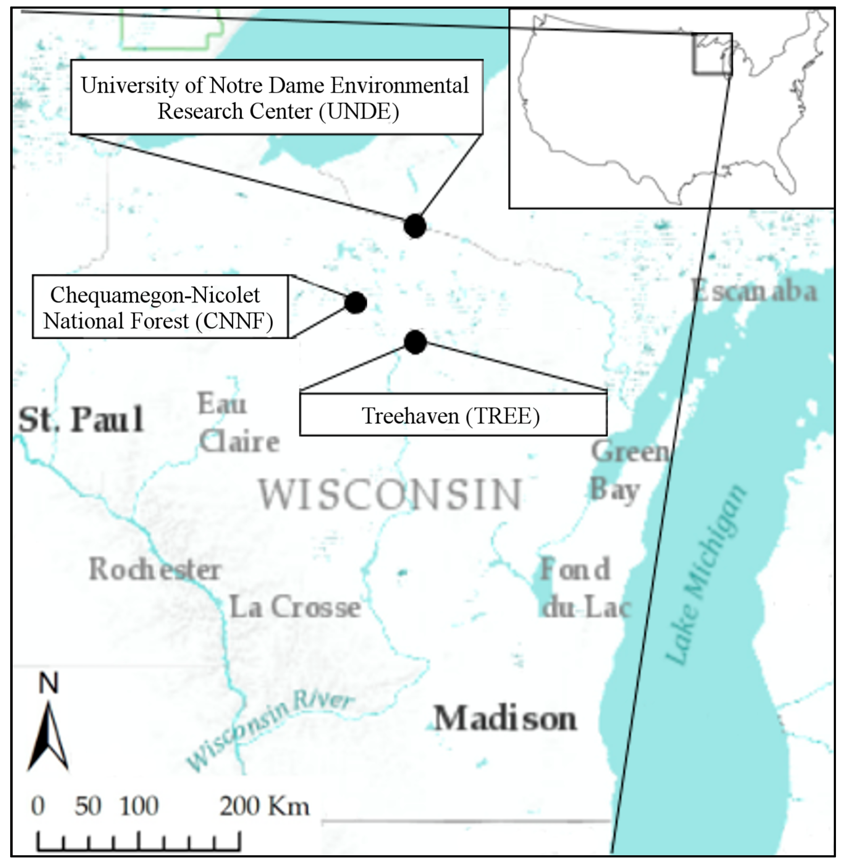
2.1. Study Area
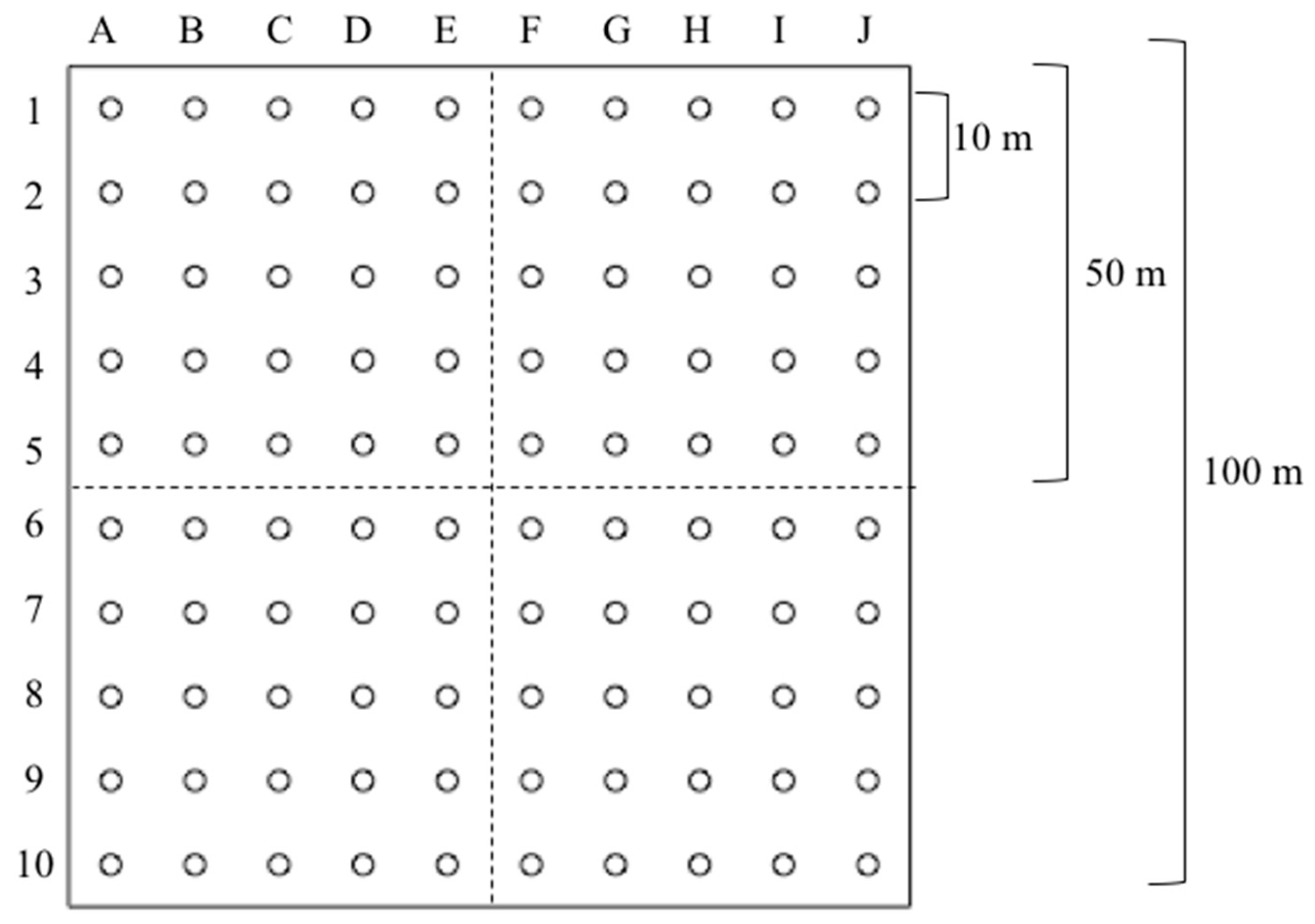
2.2. Data Source and Collection
2.3. Data Preparation
2.4. Modeling
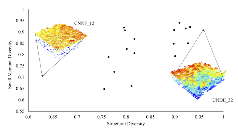
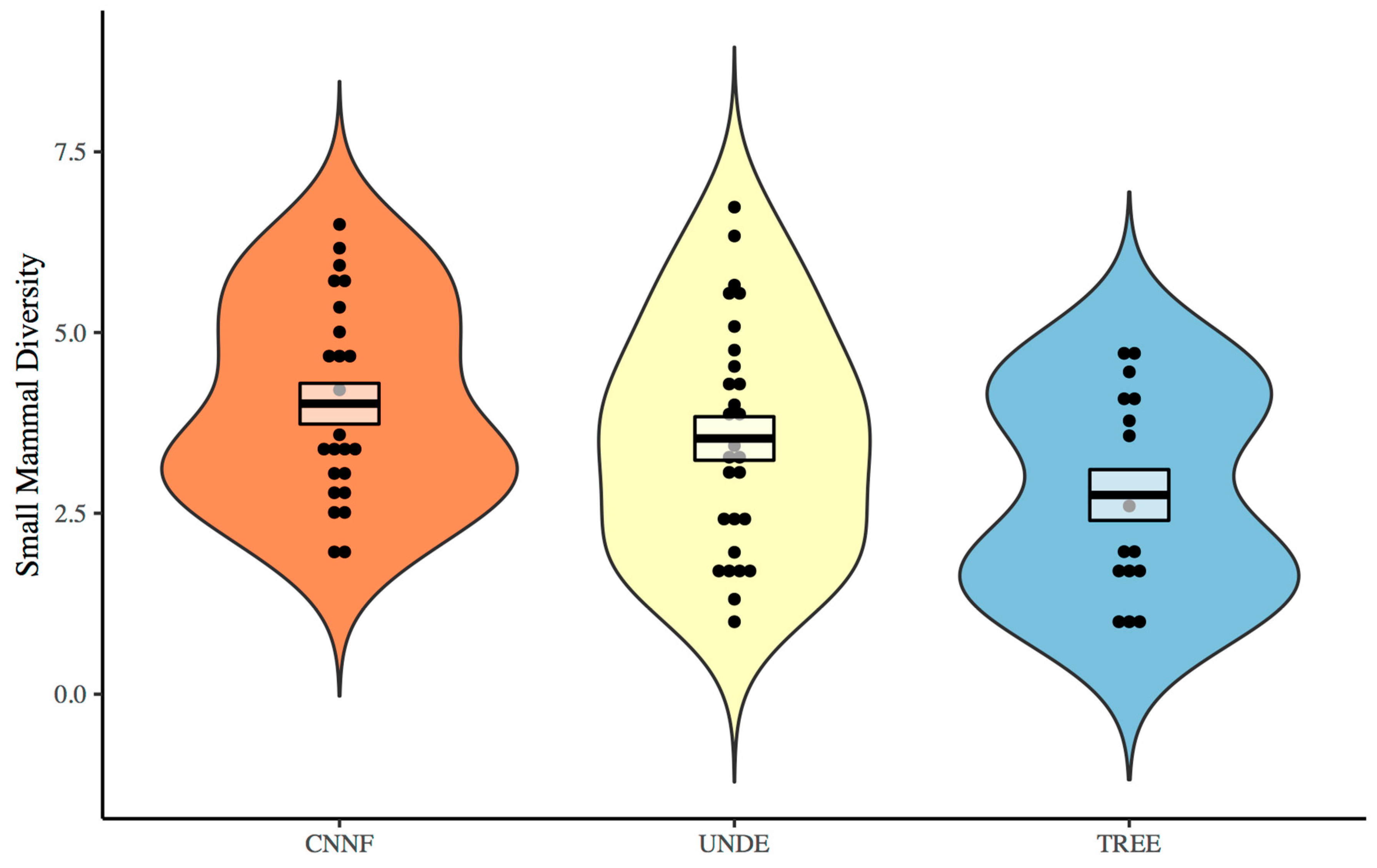
3. Results
4. Discussion
5. Conclusions
Supplementary Materials
Author Contributions
Funding
Acknowledgments
Conflicts of Interest
References
- MacAthur, R.H.; MacAthur, J. On bird species diversity. Ecology 1961, 42, 594–598. [Google Scholar] [CrossRef]
- Tews, J.; Brose, U.; Grimm, V.; Tielbörger, K.; Wichmann, M.C.; Schwager, M.; Jeltsch, F. Animal species diversity driven by habitat heterogeneity/diversity: The importance of keystone structures. J. Biogeogr. 2004, 31, 79–92. [Google Scholar] [CrossRef]
- Coops, N.C.; Tompaski, P.; Nijland, W.; Rickbeil, G.J.M.; Nielsen, S.E.; Bater, C.W.; Stadt, J.J. A forest structure habitat index based on airborne laser scanning data. Ecol. Indic. 2016, 67, 346–357. [Google Scholar] [CrossRef]
- Vogeler, J.C.; Cohen, W.B. A review of the role of active remote sensing and data fusion for characterizing forest in wildlife habitat models. Span. Assoc. Remote Sens. 2016, 1–14. [Google Scholar] [CrossRef]
- Lindberg, E.; Roberge, J.-M.; Johansson, T.; Hjältén, J. Can airborne laser scanning (ALS) and forest estimates derived from satellite images be used to predict abundance and species richness of birds and beetles in boreal forest? Remote Sens. 2015, 7, 4233–4252. [Google Scholar] [CrossRef]
- Sullivan, T.P.; Sullivan, D.S.; Lindgren, P.M.F. Small mammals and stand structure in young pine, seed-tree, and old-growth forest, southwest Canada. Ecol. Appl. 2000, 10, 1367–1383. [Google Scholar] [CrossRef]
- Thibault, K.M.; Tsau, K.; Springer, Y.; Knapp, L. TOS Protocol and Procedure: Small Mammal Sampling; revision J; NEON.DOC.000481; National Ecological Observatory Network: Boulder, CO, USA, 2017. [Google Scholar]
- Ecke, F.; Löfgren, O.; Sörlin, D. Population dynamics of small mammals in relation to forest age and structural habitat factors in northern Sweden. J. Appl. Ecol. 2002, 39, 781–792. [Google Scholar] [CrossRef]
- Fuller, A.K.; Harrison, D.J.; Lachowski, H.J. Stand scale effects of partial harvesting and clearcutting on small mammals and forest structure. For. Ecol. Manag. 2004, 191, 373–386. [Google Scholar] [CrossRef]
- Stephens, R.B.; Anderson, E.M. Habitat associations and assemblages of small mammals in natural plant communities of Wisconsin. J. Mammal. 2014, 95, 404–420. [Google Scholar] [CrossRef]
- Jaime-González, C.; Acebes, P.; Mateos, A.; Mezquida, E.T. Bridging gaps: On the performance of airborne LiDAR to model wood mouse-habitat structure relationships in pine forests. PLoS ONE 2017, 12, e0182451. [Google Scholar] [CrossRef]
- Campos, V.E.; Gatica, G.; Bellis, L.M. Remote sensing variables as predictors of habitat suitability of the viscacha rat (Octomys mimax), a rock-dwelling mammal living in a desert environment. Mammal Res. 2015, 60, 117–126. [Google Scholar] [CrossRef]
- Hatten, J.R. Mapping and monitoring Mount Graham red squirrel habitat with Lidar and Landsat imagery. Ecol. Model. 2014, 289, 106–123. [Google Scholar] [CrossRef]
- Wang, B.C.; Smith, T.B. Closing the seed dispersal loop. Trends Ecol. Evol. 2002, 17, 379–385. [Google Scholar] [CrossRef]
- Moorhead, L.C.; Souza, L.; Habeck, C.W.; Lindroth, R.L.; Classen, A.T. Small mammal activity alters plant community composition and microbial activity in an old-field ecosystem. Ecosphere 2017, 8, e01777. [Google Scholar] [CrossRef]
- Brown, J.H.; Heske, E.J. Control of a desert-grassland transition by a keystone rodent guild. Science 1990, 250, 1705–1707. [Google Scholar] [CrossRef] [PubMed]
- Gorini, L.; Linnell, J.D.C.; May, R.; Panzacchi, M.; Boitani, L.; Odden, M.; Nilsen, E.B. Habitat heterogeneity and mammalian predator-prey interactions. Mammal Rev. 2012, 42, 55–77. [Google Scholar] [CrossRef]
- Hooper, D.U.; Chapin, F.S.; Ewel, J.J.; Hector, A.; Inchausti, P.; Lavorel, S.; Lawton, J.H.; Lodge, D.M.; Loreau, M.; Naeem, S.; et al. Effects of biodiversity on ecosystem functioning: A consensus of current knowledge. Ecol. Monogr. 2005, 75, 3–35. [Google Scholar] [CrossRef]
- Tschumi, M.; Ekroos, J.; Hjort, C.; Smith, H.G.; Birkhofer, K. Predation-mediated ecosystem services and disservices in agricultural landscapes. Ecol. Appl. 2018, 28, 2109–2118. [Google Scholar] [CrossRef]
- Simonson, W.D.; Allen, H.D.; Coomes, D.A. Applications of airborne lidar for the assessment of animal species diversity. Methods Ecol. Evol. 2014, 5, 719–729. [Google Scholar] [CrossRef]
- Burns, K.J. Treehaven Experimental Forest Land Management Plan; UW-Stevens Point College of Natural Resources: Stevens Point, WI, USA, 2009. [Google Scholar]
- National Ecological Observatory Network Field Sites Information. Available online: https://www.neonscience.org/field-sites/ (accessed on 20 April 2019).
- National Forest Service. Management Area Direction; National Forest Service: Rhinelander, WI, USA, 2004.
- National Ecological Observatory Network. Data Product: TOS Sampling Site Locations. Available online: https://www.neonscience.org/data/spatial-data-maps/ (accessed on 4 March 2018).
- National Ecological Observatory Network. Data Products: DP3.30003, DP1.10072. 2018. Available online: http://data.neonscience.org (accessed on 4 March 2018).
- Krause, K.; Goulden, T. NEON L0-to-L1 Discrete Return LiDAR Algorithm Theoretical Basis Document; revision A; NEON.DOC.001292; National Ecological Observatory Network: Boulder, CO, USA, 2015. [Google Scholar]
- Goulden, T.; Hass, B. NEON AOP LMS QA/QC Report for Domain 05; National Ecological Observatory Network: Boulder, CO, USA, 2016. [Google Scholar]
- Goulden, T.; Hass, B. NEON AOP QA Report for Domain 5; National Ecological Observatory Network: Boulder, CO, USA, 2016. [Google Scholar]
- Goulden, T. NEON Elevation (DTM and DSM) Algorithm Theoretical Basis Document; National Ecological Observatory Network: Boulder, CO, USA, 2019. [Google Scholar]
- Azuaje, E.; Jones, K.; Barnett, D.; Meier, C.; Krouss, R.; McKay, J. TOS Protocol and Procedure: Plot Establishment Revision D; National Ecological Observatory Network: Boulder, CO, USA, 2015. [Google Scholar]
- Haskell, J.P.; Ritchie, M.E.; Olff, H. Fractal geometry predicts verying body size scaling relationships for mammal and bird home ranges. Nature 2002, 418, 527–530. [Google Scholar] [CrossRef]
- Kellner, K.F.; Urban, N.A.; Swihart, R.K. Short-term responses of small mammals to timber harvest in the United States Central Hardwood Forest Region. J. Wildl. Manag. 2013, 77, 1650–1663. [Google Scholar] [CrossRef]
- Roussel, J.-R.; Auty, D. lidR: Airborne LiDAR Data Manipulation and Visualization for Forestry Applications. R Package Version 1.4.1. 2018. Available online: https://CRAN.R-project.org/package=lidR (accessed on 20 April 2019).
- R Core Team. R: A Language and Environment for Statistical Computing; R Foundation for Statistical Computing: Vienna, Austria, 2018. [Google Scholar]
- Hijmans, R.J. raster: Geographic Data Analysis and Modeling. R Package Version 3.0.2. Available online: https://CRAN.R-project.org/package=raster (accessed on 20 April 2019).
- Hill, R.A.; Hinsley, S.A. Airborne lidar for woodland habitat quality monitoring: Exploring the significance of lidar data characteristics when modelling organism-habitat relationships. Remote Sens. 2015, 7, 3446–3466. [Google Scholar] [CrossRef]
- Falkowski, M.J.; Smith, A.M.S.; Hudak, A.T.; Gessler, P.E.; Vierling, L.A.; Crookston, N.L. Automated estimation of individual conifer tree height and crown diameter via two-dimensional spatial wavelet analysis of lidar data. Can. J. Remote Sens. 2005, 32, 153–161. [Google Scholar] [CrossRef]
- Pretzsch, H. Description and analysis of stand structures. In Forest Dynamics, Growth and Yield; Springer: Berlin/Heidelberg, Germany, 2009; pp. 223–289. [Google Scholar]
- Campbell, M.J.; Dennison, P.E.; Hudak, A.T.; Parham, L.M.; Butler, B.W. Quantifying understory vegetation density using small-footprint airborne lidar. Remote Sens. Environ. 2018, 215, 330–342. [Google Scholar] [CrossRef]
- van Ewijk, K.Y.; Treitz, P.M.; Scott, N.A. Characterizing forest succession in central Ontario using Lidar-derived Indices. Photogramm. Eng. Remote Sens. 2013, 77, 261–269. [Google Scholar] [CrossRef]
- Pallmann, P.; Schaarschmidt, F.; Hothorn, L.; Fischer, C.; Nacke, H.; Priesnitz, K.U.; Schork, N. Testing a user-defined selection of diversity indices. Mol. Ecol. Res. 2012, 12, 1068–1078. [Google Scholar] [CrossRef] [PubMed]
- Jost, L. Entropy and diversity. Oikos 2006, 113, 363–375. [Google Scholar] [CrossRef]
- Jost, L. Partitioning diversity into independent alpha and beta components. Ecology 2007, 88, 2427–2439. [Google Scholar] [CrossRef]
- Calcagno, V. glmulti: Model selection and multimodel inference made easy 2013. R Package Version 2018, 1, 498. [Google Scholar]
- Anderson, J.R.; Hardy, E.E.; Roach, J.T.; Witmer, R.E. A Land Use and Land Cover Classification System for Use with Remote Sensor Data; US Government Printing Office: Alexandria, VA, USA, 1976.
- Yang, L.; Jin, S.; Danielson, P.; Homer, C.; Gass, L.; Bender, S.M.; Case, A.; Costello, C.; Dewitz, J.; Fry, J.; et al. A new generation of the United States National Land Cover Database: Requirements, research priorities, design, and implementation strategies. ISPRS J. Photogramm. Remote Sens. 2018, 146, 108–123. [Google Scholar] [CrossRef]
- Burnham, K.P.; Anderson, D.D. Model Selection and Multimodel Inference: A Practical Information-Theoretic Approach, 2nd ed.; Springer: New York, NY, USA, 2002; ISBN 0387953647. [Google Scholar]
- Buckland, S.T.; Burnham, K.P.; Augustin, N.H. Model selection: An integral part of inference. Biometrics 1997, 53, 603–618. [Google Scholar] [CrossRef]
- Clawges, R.; Vierling, K.; Vierling, L.; Rowell, E. The use of airborne lidar to assess avian species diversity, density, and occurrence in a pine/aspen forest. Remote Sens. Environ. 2008, 112, 2064–2073. [Google Scholar] [CrossRef]
- Goetz, S.; Steinberg, D.; Dubayah, R.; Blair, B. Laser remote sensing of canopy habitat heterogeneity as a predictor of bird species richness in an eastern temperate forest, USA. Remote Sens. Environ. 2007, 108, 254–263. [Google Scholar] [CrossRef]
- Froidevaux, J.S.P.; Zellweger, F.; Bollmann, K.; Jones, G.; Obrist, M.K. From field surveys to LiDAR: Shining a light on how bats respond to forest structure. Remote Sens. Environ. 2016, 175, 242–250. [Google Scholar] [CrossRef]
- Nelson, R.; Keller, C.; Ratnaswamy, M. Locating and estimating the extent of Delmarva fox squirrel habitat using an airborne LiDAR profiler. Remote Sens. Environ. 2005, 96, 292–301. [Google Scholar] [CrossRef]
- Carey, A.B.; Wilson, S.M. Induced spatial heterogeneity in forest canopies: Responses of small mammals. J. Wildl. Manag. 2010, 65, 1014–1027. [Google Scholar] [CrossRef]
- Carey, A.B.; Kershner, J.; Biswell, B.; Dominguez de Toledo, L. Ecological scale and forest development: Squirrels, dietary fungi, and vascular plants in managed and unmanaged forests. Wildl. Monogr. 1999, 142, 3–71. [Google Scholar]
- Bogdziewicz, M.; Zwolak, R. Responses of small mammals to clear-cutting in temperate and boreal forests of Europe: A meta-analysis and review. Eur. J. For. Res. 2014, 133, 1–11. [Google Scholar] [CrossRef]
- Nelson, D.L. Demographic Responses of Small Mammals to Distrurbance Induced by Forest Management. Master’s Thesis, Purdue University, West Lafayette, IN, USA, 2017. [Google Scholar]
- Martinuzzi, S.; Vierling, L.A.; Gould, W.A.; Falkowski, M.J.; Evans, J.S.; Hudak, A.T.; Vierling, K.T. Mapping snags and understory shrubs for a LiDAR-based assessment of wildlife habitat suitability. Remote Sens. Environ. 2009, 113, 2533–2546. [Google Scholar] [CrossRef]
- Srinivasan, S.; Popescu, S.C.; Eriksson, M.; Sheridan, R.D.; Ku, N.W. Terrestrial laser scanning as an effective tool to retrieve tree level height, crown width, and stem diameter. Remote Sens. 2015, 7, 1877–1896. [Google Scholar] [CrossRef]
- Zellweger, F.; De Frenne, P.; Lenoir, J.; Rocchini, D.; Coomes, D. Advances in Microclimate Ecology Arising from Remote Sensing. Trends Ecol. Evol. 2019, 34, 327–341. [Google Scholar] [CrossRef]
- Sumnall, M.; Fox, T.R.; Wynne, R.H.; Thomas, V.A. Mapping the height and spatial cover of features beneath the forest canopy at small-scales using airborne scanning discrete return Lidar. ISPRS J. Photogramm. Remote Sens. 2017, 133, 186–200. [Google Scholar] [CrossRef]
- Mitchell, B.; Walterman, M.; Mellin, T.; Wilcox, C.; Lynch, A.M.; Anhold, J.; Falk, D.A.; Koprowski, J.; Laes, D.; Evans, D.; et al. Mapping Vegetation Structure in the Pinaleño Mountains Using Lidar—Phase 3: Forest Inventory Modeling; Department of Agriculture, Forest Service, Remote Sensing Applications Center: Salt Lake City, UT, USA, 2012.
- Ecke, F.; Lofgren, O.; Hornfeldt, B.; Eklund, U.; Ericsson, P.; Sorlin, D. Abundance and Diversity of Small Mammals in Relation to Structural Habitat Factors. Ecol. Bull. 2001, 49, 165–171. [Google Scholar]
- Fischer, J.; Lindenmayer, D.B. Landscape modification and habitat fragmentation: A synthesis. Glob. Ecol. Biogeogr. 2007, 16, 265–280. [Google Scholar] [CrossRef]


| Predictor | Metric Calculation | Dimension | Mean | St. Dev. | Range |
|---|---|---|---|---|---|
| Canopy Height (m) | Mean of the canopy height model | Average | 13.62 | 5.23 | 4.81–21.86 |
| Cover | Number of first returns above 2 m/total number of first returns | Vertical | 0.87 | 0.11 | 0.62–0.99 |
| Understory Contribution | Number of returns above 0.2 m and less than 5 m/total number of returns | Horizontal | 0.34 | 0.21 | 0.05–0.70 |
| Canopy Complexity | Coefficient of variation of height for first returns above 5 m | Vertical | 0.89 | 0.09 | 0.65–0.98 |
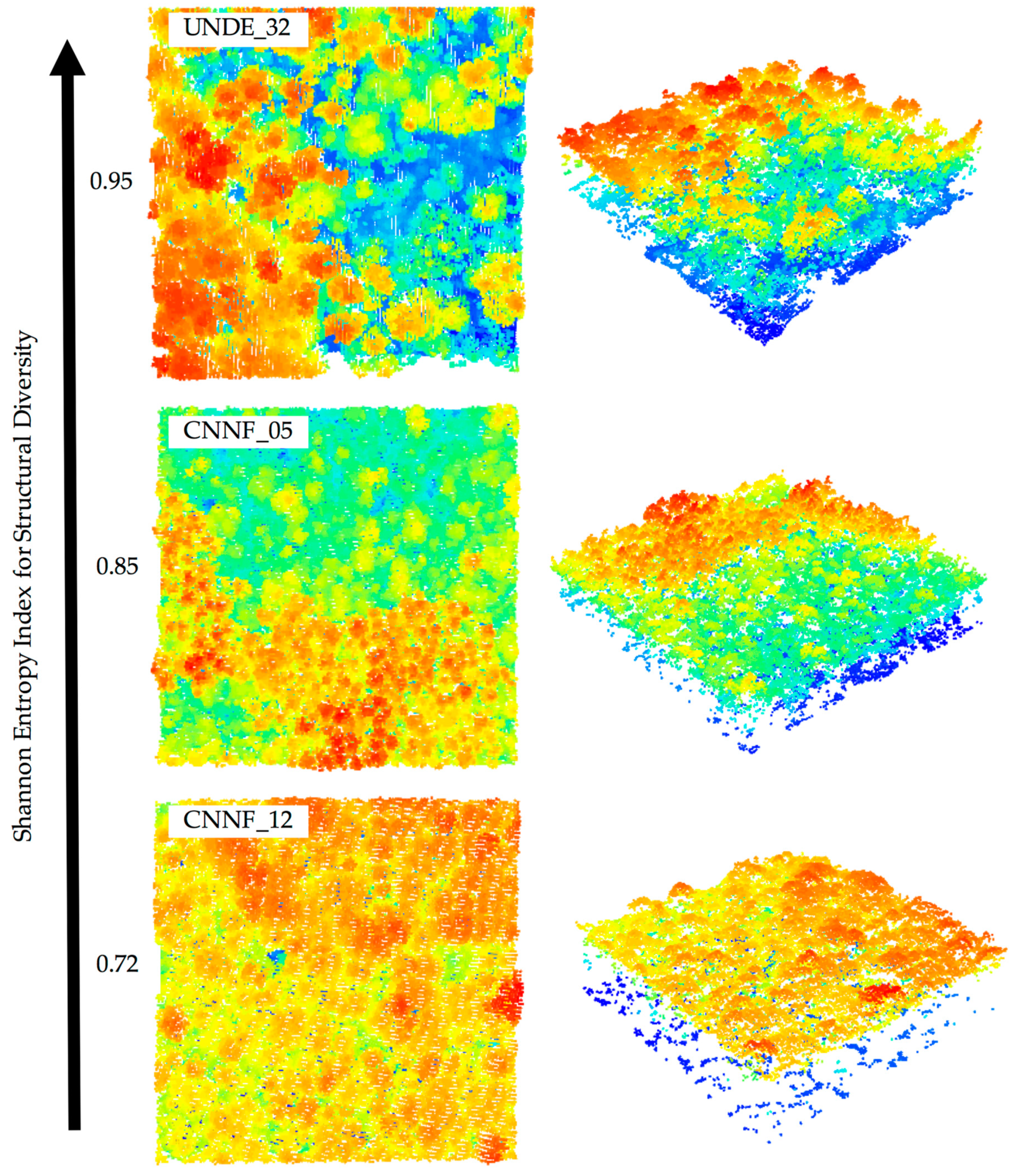
| Structural Diversity | Shannon structural entropy index in 1 m bins | Vertical | 0.84 | 0.07 | 0.72–0.95 |
| Model Name | df | logLik | AICc | Δ AICc | w |
|---|---|---|---|---|---|
| Structural Diversity + Cover | 4 | −27.46 | 66.26 | 0.00 | 0.19 |
| Structural Diversity + Canopy Height | 4 | −27.62 | 66.58 | 0.32 | 0.16 |
| Structural Diversity | 3 | −29.51 | 66.86 | 0.60 | 0.14 |
| Structural Diversity + Understory Contribution | 4 | −28.09 | 67.51 | 1.25 | 0.10 |
| Cover + Canopy Complexity | 4 | −28.58 | 68.49 | 2.23 | 0.06 |
| Model Name | df | logLik | AICc | Δ AICc | w |
|---|---|---|---|---|---|
| Structural Diversity + Cover + Canopy Complexity + Site | 7 | −105.72 | 227.30 | 0.00 | 0.17 |
| Structural Diversity + Cover + Site | 6 | −107.83 | 229.04 | 1.75 | 0.07 |
| Structural Diversity + Cover | 5 | −109.07 | 229.10 | 1.81 | 0.07 |
| Structural Diversity | 3 | −111.41 | 229.19 | 1.90 | 0.06 |
| Structural Diversity + Site | 5 | −109.16 | 229.28 | 1.98 | 0.06 |
| Parameter | Estimate | Variance | Importance |
|---|---|---|---|
| Plot | |||
| Structural Diversity | 0.532 | 0.324 | 0.83 |
| Canopy Height | −0.177 | 0.323 | 0.37 |
| Cover | −0.112 | 0.228 | 0.33 |
| Understory Contribution | 0.084 | 0.207 | 0.25 |
| Canopy Complexity | 0.080 | 0.252 | 0.23 |
| Site (TREE, UNDE) | 0.001, 0.001 | 0.031, 0.034 | 0.02 |
| Subplot | |||
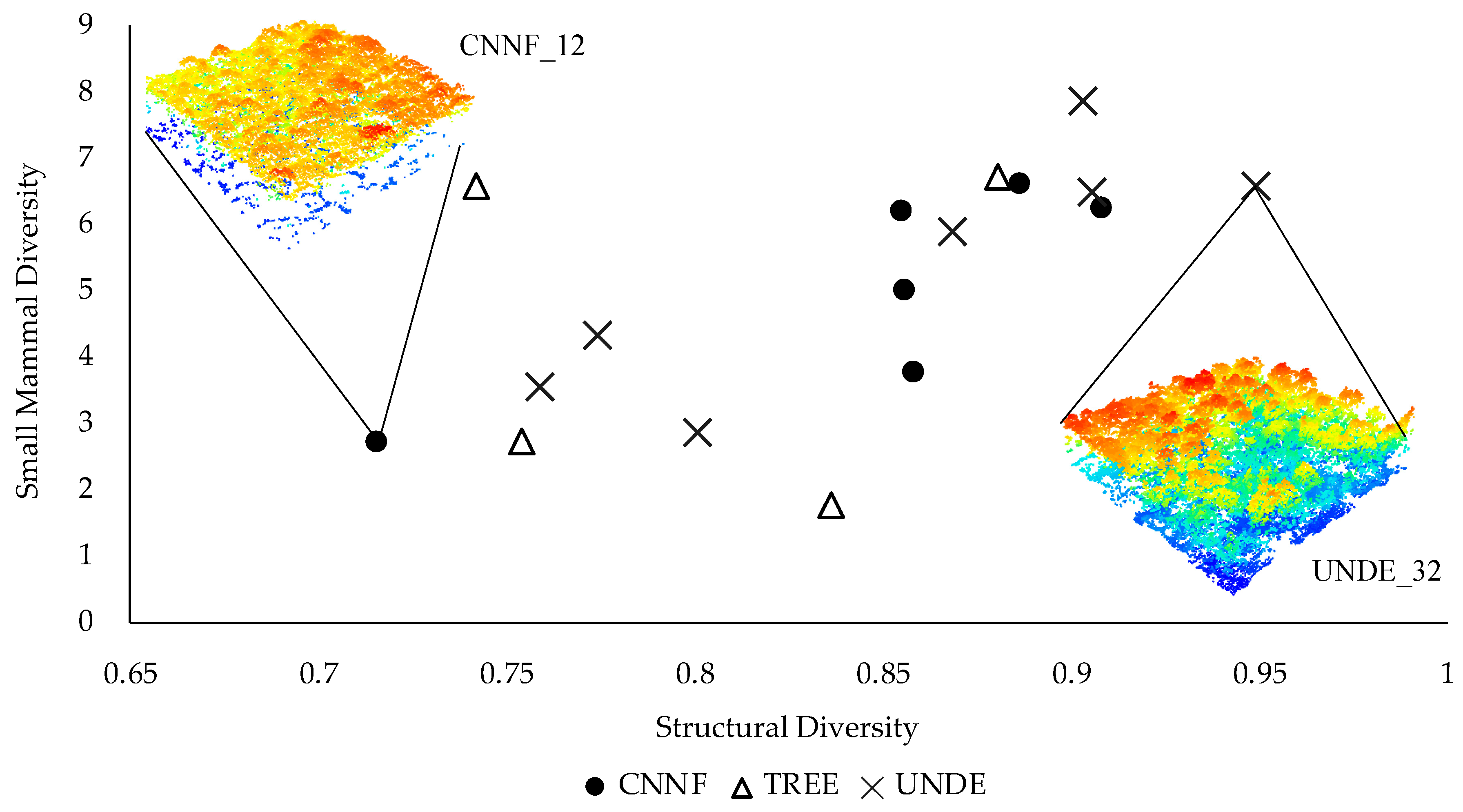
| Structural Diversity | 0.573 | 0.119 | 1.00 |
| Cover | −0.186 | 0.209 | 0.61 |
| Site (TREE, UNDE) | −0.159, −0.07 | 0.159, 0.105 | 0.60 |
| Canopy Complexity | 0.144 | 0.186 | 0.54 |
| Canopy Height | −0.034 | 0.124 | 0.30 |
| Understory Contribution | 0.002 | 0.075 | 0.25 |
© 2019 by the authors. Licensee MDPI, Basel, Switzerland. This article is an open access article distributed under the terms and conditions of the Creative Commons Attribution (CC BY) license (http://creativecommons.org/licenses/by/4.0/).
Share and Cite
Schooler, S.L.; Zald, H.S.J. Lidar Prediction of Small Mammal Diversity in Wisconsin, USA. Remote Sens. 2019, 11, 2222. https://doi.org/10.3390/rs11192222
Schooler SL, Zald HSJ. Lidar Prediction of Small Mammal Diversity in Wisconsin, USA. Remote Sensing. 2019; 11(19):2222. https://doi.org/10.3390/rs11192222
Chicago/Turabian StyleSchooler, Sarah L., and Harold S. J. Zald. 2019. "Lidar Prediction of Small Mammal Diversity in Wisconsin, USA" Remote Sensing 11, no. 19: 2222. https://doi.org/10.3390/rs11192222
APA StyleSchooler, S. L., & Zald, H. S. J. (2019). Lidar Prediction of Small Mammal Diversity in Wisconsin, USA. Remote Sensing, 11(19), 2222. https://doi.org/10.3390/rs11192222