DepthLearn: Learning to Correct the Refraction on Point Clouds Derived from Aerial Imagery for Accurate Dense Shallow Water Bathymetry Based on SVMs-Fusion with LiDAR Point Clouds

Abstract

The determination of accurate bathymetric information is a key element for near offshore activities; hydrological studies, such as coastal engineering applications, sedimentary processes, hydrographic surveying, archaeological mapping and biological research. Through structure from motion (SfM) and multi-view-stereo (MVS) techniques, aerial imagery can provide a low-cost alternative compared to bathymetric LiDAR (Light Detection and Ranging) surveys, as it offers additional important visual information and higher spatial resolution. Nevertheless, water refraction poses significant challenges on depth determination. Till now, this problem has been addressed through customized image-based refraction correction algorithms or by modifying the collinearity equation. In this article, in order to overcome the water refraction errors in a massive and accurate way, we employ machine learning tools, which are able to learn the systematic underestimation of the estimated depths. In particular, an SVR (support vector regression) model was developed, based on known depth observations from bathymetric LiDAR surveys, which is able to accurately recover bathymetry from point clouds derived from SfM-MVS procedures. Experimental results and validation were based on datasets derived from different test-sites, and demonstrated the high potential of our approach. Moreover, we exploited the fusion of LiDAR and image-based point clouds towards addressing challenges of both modalities in problematic areas.

1. Introduction

Through-water depth determination from aerial imagery is a much more time consuming and costly process compared to similar onshore mapping tasks. However, it is still a more efficient operation than ship-borne echo sounding methods or underwater photogrammetric methods [1], especially when it comes to shallower (less than 10 m depth) clear water areas. Additionally, using imagery data, a permanent record of other features can be obtained in the coastal region, such as tidal levels, coastal dunes, rock platforms, beach erosion, and vegetation [2]. This is the case, even though many alternatives for bathymetry [3] have been reported recently. This is especially the case for the coastal zones of up to 10 m depth, in which most of the economic activities are concentrated. Hence, this zone is prone to accretion or erosion and it is ground for development, since there is no affordable and universal solution for seamless underwater and overwater mapping. On one hand, image-based mapping techniques generally fail due to wave breaking effects and water refraction, while echo sounding techniques; on the other, fail due to the short sensor-to-object distances [4].

At the same time, bathymetric LiDAR systems with simultaneous image acquisition are a valid and very accurate, albeit expensive alternative, especially for small scale surveys. In addition, even though the image acquisition for orthophotomosaic generation in land is a solid solution when using multisensor platforms, the same cannot be said for the shallow water seabed. Despite the accurate and precise depth map provided by bathymetric LiDAR [5], the seabed orthoimage generation using the simultaneously acquired aerial imagery is not directly feasible due to the refraction effect. This leads to another missed opportunity to benefit from a unified seamless mapping process.

This work reported here is an extension of our earlier conference publication [6], by performing intensive experiments and cross-validation with additional datasets, while also employing additional reference/check points measured with a real time kinematic (RTK) GPS and dipping tape. Additionally, fusion of the LiDAR and the corrected image-based point clouds was performed.

1.1. The Impact of the Refraction Effect on Structure from Motion-Multi-View-Stereo (SfM-MVS) Procedures

Even though aerial imagery is well established for monitoring and 3D recording of dry landscapes and urban areas, when it comes to bathymetric applications, errors are introduced due, mainly, to the water refraction. According to the literature [7,8,9], thorough calibration is sufficient to correct the effects of refraction in the case of in-water photogrammetric procedures. On the contrary, in through-water (two-media) cases, the sea surface undulations due to waves [10,11] and the magnitude of refraction, which differ practically at each point of every image, lead to unstable solutions [12,13]. More specifically, according to Snell’s law, the effect of the refraction of a light beam is affected by water depth and angle of incidence of the beam in the air/water interface. The problem becomes even more complex when multi-view geometry is applied. In Figure 1, the multiple view geometry, which applies also to the aerial image datasets (UAV) imagery, is demonstrated: the erroneous, apparent depth C is calculated by the collinearity equation.

Starting from that apparent depth of a point A, its image-coordinates a₁, a₂, a_3, …, a_n, can be backtracked on images O₁, O₂, O₃, …, O_n using the standard collinearity equation. If a point has been matched successfully on the photos O₁, O₂, O₃, …, O_n, then the standard collinearity intersection would have returned the point C, which is the apparent and shallower position of point A; and in the multiple view case is the adjusted position of all the possible red dots in Figure 1, which are the intersections for each stereopair. Thus, without some form of correction, refraction produces an image and consequently a point cloud of the submerged surface which appears to lie at a shallower depth than the real surface. In the related literature, two main approaches to correct refraction in through-water photogrammetry can be found: analytical or image based [14].

1.2. Fusing Image-Based and LiDAR Seabed Point Clouds

Many issues arise regarding the fusion of the LiDAR and image-based point clouds, specifically those produced from aerial imagery while facing the refraction effect. Seabed point cloud data resulting from bathymetric LiDAR systems deliver geolocalized point clouds and correct depth information after refraction correction. However, in most of the cases, these data are quite sparse for underwater archaeological or biological research, missing the required density and RGB color information. However, nowadays, this color information seems to be very important for achieving reliable results from many machine learning and deep learning classification approaches. Moreover, LiDAR data in the very shallow nearshore zone (<2 m depth) suffer from the difficulty of extraction of the surface and bottom positions, which are typically mixed in the green LiDAR signal [15]; however, recent approaches [16] show promise toward meeting this challenge. On the contrary, although image-based point clouds, generated through SfM-MVS processes, have color information, they suffer from the refraction effect described in 1.1. Moreover, previous research [6] demonstrated that image-based methods for seabed point cloud generation, are not achieving great results in sandy seabed and non-static areas covered with seagrass, since the texture of the images in these areas is quite poor and area based least squares matching and correlation algorithms fail, leading to the lack of correspondences in these areas. Additionally, sun glint on the water surface, may compromise the results. However, they carry much information important for exploiting them in the recent classification-and-semantic segmentation approaches of seabed morphology, marine flora and fauna, and coral reefs [17].

Fusion of these two types of data will facilitate a better sensing and understanding of the seabed of the non-turbid shallow water bodies, exploiting the complementary attributes of both point cloud sources. However, by not dealing with the refraction effect, and consequently, the erroneous depth information on the initial image-based point clouds in a robust and reliable way, like the one presented here, fusion is impossible due to the incompatibility of the point clouds.

1.3. Contribution of the Present Research

In this work, a new approach to address the systematic refraction errors of point clouds derived from SfM-MVS procedures in a massive and accurate way is proposed. The developed technique is based on machine learning tools which can accurately recover shallow bathymetric information from aerial image datasets (UAV imagery in our case) over a calm water surface, supporting several coastal engineering applications. In particular, the goal was to deliver image-based point clouds with accurate depth information by training models which estimate the correct depth from the systematic differences between image-based products and bathymetric LiDAR point clouds. The latter is currently considered the “golden standard” for shallow water depths. To this end, a linear support vector regression (SVR) model was employed and trained to predict the actual depth Z from the apparent depth Z₀ of a point, from the image-based point cloud. In order to demonstrate that the trained models have significant potential for applications over different areas and shallow waters, and that a predicted model can be used in areas where LiDAR data are not available, training and testing processes were always performed in different test sites. As such, a model trained on the image-based point cloud and the LiDAR point cloud of a test site, was tested on many other different test sites, where LiDAR data were also available but used only for evaluating the predicted depths. Consequently, the availability of a LiDAR point cloud for the depth correction in a particular site is not a prerequisite. Moreover, in this study the fusion of the LiDAR and the corrected image-based point clouds is proposed, and the experimental design and the quite promising results derived are discussed in detail.

The rest of the article is organized as follows: Section 2 presents the related work regarding refraction correction, the use of Support Vector Machines (SVMs) and regression models in bathymetry determination, and finally, the state of the art in seabed data fusion and integration. In Section 3, the datasets used are described, while in Section 4 the proposed methodology is presented and justified. In Section 5, the tests performed and the evaluations carried out are described. In Section 6, the fusion approach of the corrected image-based point cloud with the LiDAR point cloud is described. Section 7 discusses the results of the proposed method, and Section 8 concludes the paper.

2. Related Work

2.1. Analytical and Image-Based Refraction Correction

Refraction effect has driven scholars to suggest several correction models for two-media photogrammetry, most of which are dedicated to specific applications. Two-media photogrammetry is divided into through-water and in-water photogrammetry. The “through-water” term is used when the camera is above the water surface and the object is underwater, hence part of the ray is traveling through air and part of it through water. It is most commonly used in aerial photogrammetry [4] or in close range applications [13,18]. It was even argued that if the water depth to flight height ratio is considerably low, then compensation of water refraction is unnecessary [2]. However, as shown by the authors in [4], the water depth to flying height ratio is irrelevant in cases of aerial imaging, and water refraction correction is necessary. The “in-water” photogrammetry term is used when both camera and object are in the water.

Two-media photogrammetric techniques have been reported already, in the early 1960s [19,20], and the basic optical principles proved that photogrammetric processing through water is possible. In the literature, two main approaches to correct refraction in through-water photogrammetry can be found: analytical or image-based. The first approach is based on the modification of the collinearity equation [13,18,21,22,23], while the latter is based on re-projecting the original photo to correct the water refraction [4,12]. According to [14], there are two ways to analytically correct the effects of refraction in two-media photogrammetry: the deterministic (explicit) and unsettled (ambiguous and iterative). The iterative method is employed to resolve refraction, either in object space [22] or in image space [14]. In the latter case, the whole multimedia problem is simplified to the radial shift computation module [12], which is also the main concept of this study.

The two-media analytically based methods, have been used for underwater mapping using special platforms for hoisting the camera [23,24,25]. For mapping an underwater area, authors in [26] used a “floating pyramid” for lifting two cameras. The base of the pyramid was made of Plexiglas for avoiding wave effects and sun glint, which according to [27], sometimes limits the performance of two-media approaches. A contemporary, but similar approach is adopted by [18] for mapping the bottom of a river. There, the extracted digital surface model (DSM) points have been corrected from refraction effects, using a dedicated algorithm which corrects the final XYZ of the points. A Plexiglas surface was again used for hosting the control points. In [28], for modelling a scale-model rubble-mound breakwater, refraction effects were described via a linearized Taylor series, which is valid for paraxial rays. That way, a virtual principal point was defined, where all rays were converging. It has been shown that this approach offers satisfactory compensation for the two media involved.

Muslow [29] developed a general but sophisticated analytical model, as part of the bundle adjustment solution. The model allows for simultaneous determination of camera orientation, 3D object point coordinates, an arbitrary number of media (refraction) surfaces, and the determination of the corresponding refractive index. The author supported the proposed model with experimental data and a corresponding solution. Another approach [30], introduced a new 3D feature-based surface reconstruction made by using the trifocal tensor. The method was extended to multimedia photogrammetry and applied to an experiment on the photogrammetric reconstruction of fluvial sediment surfaces. In [31], authors were modelling the refraction effect to accurately measure deformations on submerged objects. They used an analytical formulation for refraction at an interface, out of which a non-linear solution approach was developed to perform stereo calibration. Aerial images have also been used for mapping the sea bottom with an accuracy of approximately 10% of the water depth in cases of clear waters and shallow depths; i.e., 5–10 m [32,33,34].

Recently, in [35] an iterative approach that calculates a series of refraction correction equations for every point/camera combination in a SfM point cloud is proposed and tested. There, for each point in the submerged portion of the SfM-resulting point cloud, the software calculates the refraction correction equations and iterates through all the possible point-camera combinations.

In [14], the authors adopt a simplified model of in-water and through-water photogrammetry by making assumptions about the camera being perpendicular to a planar interface. In [36], the authors avoided the full strict model of two-media photogrammetry if the effects could be considered as radial symmetric displacements on the camera plane—effects which could be absorbed from camera constant and radial lens distortion parameters. With the same concept, authors in [7] state that the effective focal length in underwater photogrammetry is approximately equal to the focal length in air, multiplied by the refractive index of water. This model was extended by [12], by also considering the dependency on the percentages of air and water within the total camera-to-object distance. However, these oversimplified models can only be valid for two-media photogrammetry, where the camera is strictly viewing perpendicularly onto a planar object. Obviously, this is not the general case, because the bottom and the water surfaces are seldomly flat and planar, while the photographs can be perfectly perpendicular only with sophisticated camera suspension mounts. When UAV (drone) photographs are being used to create a 3D model of the sea bottom and create the corresponding orthophotograph object [22], these assumptions are not valid. For these reasons, the proposed method in [12] was extended in [4], where the same principle was differentially applied over the entire area of the photograph. In [37] a less sophisticated approach is adopted, where the apparent water depths are multiplied by the refractive index of clear water to obtain refraction corrected water depths. Results present errors of 0.05–0.08 m, while the average water depth ranged between 0.14 m and 0.18 m, and maximum water depth between 0.50 m and 0.70 m. In [38] authors developed a refraction correction model for airborne imagery by examining the horizontal differences between the observed and true positions when objects were aligned along an airplane track or when the incident angles were identical. The procedure was applied in real world and the comparison of the corrected depths with measured depths at 658 points showed a mean error and standard deviation of 0.06 m and 0.36 m, respectively, for a measured depth range of 3.4 m to 0.2 m. The same approach was also applied in [39] for refraction correction on bathymetry derived from a WorldView-2 stereopair. Results suggested a mean error of 0.03 m and an RMSE of 1.18 m. In [40], authors presented a first approach for simultaneously recovering the 3D shape of both the wavy water surface and the moving underwater scene, and tested over both synthetic and real data. There, after acquiring the correspondences across different views, the unknown water surface and underwater scene were estimated through minimizing an objective function under a normal consistency constraint. In [41], authors attempt to address the accurate mapping of shallow water bathymetry by comparing three approaches: one based on echo sounding, and two based on photogrammetry—bathymetric SfM and optical modelling, also referred to as the spectral depth approach or optical-empirical modelling. The bathymetric SfM exploited here is the one described in [35]. The results from the photogrammetric methods suggest that the quality of the bathymetric SfM was highly sensitive to flow turbidity and color, and therefore, depth. However, it suffers less from substrate variability, turbulent flow, or large stones and cobbles on the riverbed than optical modelling. Color and depth did affect optical model performance, but clearly less than the bathymetric SfM. Finally, in a recent work presented in [42] and extended in [43] an investigation on the potential of through-water DIM (dense image matching) for the high resolution mapping of generally low textured shallow water areas is presented. For correcting the refraction effect, after extracting a water surface model from bathymetric LiDAR data, the approach presented in [44] is adopted. In the case study presented there, the DIM-derived underwater surfaces of coastal and inland water bodies are compared to concurrently acquired bathymetric LiDAR data. Results present deviations in the decimeter-range over depths of more than 5 m compared to the laser data as reference.

Even though some of the above methodologies and models produce quite accurate results, most of them are dependent on a lot of parameters, such as the interior and the exterior orientation of the camera and the water surface. On the contrary, the solution proposed in this article is independent from these parameters, requiring only an image-based point cloud for its implementation, offering flexibility to the available data, as well as a fast solution, compared to the above methods.

2.2. Image-Based Bathymetry Estimation Using Machine Learning and Simple Regression Models

Even though the presented approach is the only one dealing with UAV imagery and dense point clouds resulting from the SfM-MVS processing, there are a small number of single image approaches for bathymetry retrieval using satellite imagery. Most of those methods are based on the relationship between the reflectance and the depth. Some of them exploit an SVM system to predict the correct depth [45,46]; experiments therein showed that the localized model reduced the bathymetry estimation error by 60% from a Root Mean Square Error (RMSE) of 1.23 m to 0.48 m. In [47] a methodology is introduced using an ensemble learning (EL) fitting algorithm of least squares boosting (LSB) for bathymetric map calculations in shallow lakes from high resolution satellite images and water depth measurement samples using an echo sounder. The bathymetric information retrieved from the three methods [45,46,47] was evaluated using echo sounder data. The LSB fitting ensemble resulted in an RMSE of 0.15 m where the Principal Component Analysis (PCA) and Generalized Linear Model (GLM) yielded RMSEs of 0.19 m and 0.18 m respectively, over shallow water depths less than 2 m. In [48], among other pre-processing steps, authors implemented and compared four different empirical SDB (satellite-derived bathymetry) approaches to derive bathymetry from pre-processed Google Earth Engine Sentinel-2 composites. Empirical SDB methods require certain bands in the visible wavelength—with blue and green being the most widely used—and a set of known in situ depths as the only inputs in simple or multiple linear regressions, which leads to bathymetry estimations in a given area. Accuracies of the calibrated model in the two validation sites reached an RMSE of 1.67 m. In [49], a multiple regression bathymetry model was employed for substrate mapping in shallow fluvial systems having depth <1 m. To do so the authors analyzed spectroscopic measurements in a hydraulic laboratory setting, simulated water-leaving radiances under various optical scenarios and evaluated the potential to map bottom composition from a WorldView-3 image. In [50], authors compare the potential of through-water photogrammetry and spectral depth approaches to extract water depth for environmental applications. Imagery and cross sections were collected over a 140 m reach of a river of a maximum depth of 1.2 m approximately, using a UAV and real time kinematic (RTK)-GPS. There, for the site-specific refraction correction method, sparse calibration data resulting from two-thirds of the cross-section data were used to calibrate a simple linear regression equation between the predicted and measured water depths, and one-third of the data were used for validation and testing. This method achieved a mean error of 0.17–0.18 m at a maximum depth of 1.2 m. In [51], authors examine the relatively high-resolution Multispectral Instrument (MSI) onboard Sentinel-2A and the Moderate-Resolution Ocean and Land Color Instrument onboard Sentinel-3A for generating bathymetric maps through a conventional ratio transform model in environments with some turbidity. The MSI retrieved bathymetry at 10 m spatial resolution with errors of 0.58 m, at depths ranging between 0 and 18 m (limit of lidar survey) at the first test site, and of 0.22 m at depths ranging between 0 and 5 m in the second test site, in conditions of low turbidity. In [52], authors focused on defining the limits of spectrally based mapping in a large river. They used multibeam echosounder (MBES) surveys and hyperspectral images from a deep, clear-flowing channel to develop techniques for inferring the maximum detectable depth directly from an image and identifying optically deep areas that exceed the maximum depth. There, results suggest a limit of 9.5 m depth.

The bathymetric mapping approach presented in this article differs from other similar approaches as far as the type of the primary data used is concerned. Regarding the approaches using satellite imagery, these are not based in SfM-MVS processing but in empirical SDB or model-based bathymetry, in order to predict the depth according to the spectral value. However, in most of the studies presented in these articles, with the exception of [48], test and evaluation steps are implemented on percentages of the same test site and at very shallow depths, leading to site-specific approaches. In most cases, the 80% of the available data is used for training the model while the remaining 20% is used for evaluation. On the contrary, in this article, three different test sites are used for training, testing, and cross-evaluating the proposed approach, suggesting a more global and data independent solution to the refraction problem affecting the aerial image-based seabed mapping.

2.3. Fusing Seabed Point Clouds

Even though aerial point cloud fusion tends to be a well-established methodology [53] for in land and dry scenes, few works exist in the literature addressing seabed point cloud fusion using at least one overwater source of data, such as airborne LiDAR or UAV imagery. In [54], authors suggested an approach for integrating two types of unmanned aerial system (UAS) sampling techniques. The first, couples a small UAS to an echosounder attached to a miniaturized boat for surveying submerged topography in deeper waters, while the second uses SfM-MVS to cover shallower water areas not covered by the echosounder. A zonal, adaptive sampling algorithm was developed and applied to the echosounder data to densify measurements where the standard deviation of clustered points was high. The final product consisted of a smooth DSM of the bottom with water depths ranging from 0 m to 5.11 m. In [55], authors developed and evaluated a hybrid approach to capture the morphology of a river that combines LiDAR topography with spectrally based bathymetry. The key innovation presented in that paper was a framework for mapping bed elevations within the active channel by merging LiDAR-derived water surface elevations with bathymetric information inferred from optical images. In that study, highly turbid water conditions dictated a positive relation between green band radiance and depth. In [56], authors presented a method to fill bathymetric data holes through data merging and interpolation in order to produce a complete representation of a coral habitat. The method first merges ancillary digital sounding data with airborne bathymetric LiDAR data in order to populate data points in all areas, but particularly those with data holes. Then, the generation of an elevation surface by spatial interpolation based on the merged data points obtained in the first step takes place. In that work, four interpolation techniques, including Kriging, natural neighbor, spline, and inverse distance weighting were implemented and evaluated on their ability to accurately and realistically represent the shallow-water bathymetry of the study area. However, the natural neighbor technique was found to be the most effective one. The enhanced DEM was used in conjunction with IKONOS imagery to produce a complete, three-dimensional visualization of the study area. In [57], a new approach to shallow water bathymetry mapping, integrating hyperspectral images and sparse sonar data, was proposed. The approach includes two main steps: the dimensional reduction of Hyperion images and the interpolation of sparse sonar data. Results suggest that the bathymetry retrieved using this method is more precise than that retrieved using common interpolation methods. Finally, in one of the most completed works found in the literature [58] in terms of exploited sensors, authors proposed a framework to fill the white ribbon area of a coral reef system by integrating multiple elevation data sets acquired by a suite of remote-sensing technologies into a seamless DEM. There, a range of data sets are integrated, including GPS elevation points, topographic and bathymetric LiDAR, single and multibeam echo-soundings, nautical charts, and bathymetry derived from optical remote-sensing imagery. The proposed framework ranks data reliability internally, thereby avoiding the requirements to quantify absolute error, and results in a high-resolution, seamless product.

Although the above presented approaches do deal with the fusion of bathymetric data, they do not deal with the fusion of aerial image-based point clouds resulting from SfM-MVS processes with LiDAR point clouds. The most probable reason for this might be the strong refraction effect which affects photogrammetric bathymetry, leading to great errors, and as a result, great differences and depth inconsistencies compared to the LiDAR data.

3. Datasets and Pre-Processing

The proposed methodology has been applied to three different test areas with datasets acquired for real world shallow bathymetry mapping tasks. The image-based point clouds for this study were derived using a commercial software implementing standard SfM-MVS algorithms. The particular software implementation does not affect their qualities and it should be noted that they could be produced in a similar way using any other commercial or open source automated photogrammetric software without employing any water refraction compensation.

It should be kept in mind that, since wind affects the sea surface with wrinkles and waves, the water surface needs to be as flat as possible at the time of the photography, in order to have best sea bottom visibility and follow the geometric assumption of a flat-water surface. In the case of a wavy surface, errors would be introduced [11,12] and the relationship of the real and the apparent depths would be more scattered, affecting, to some extent, the training and the fitting of the model. Furthermore, water should not be very turbid to ensure a clear view to the bottom. Obviously, water turbidity and water visibility are additional restraining factors. Just like in any common automated photogrammetric project, the sea bottom must present texture or some kind of random pattern to ensure point detection and matching. This means that automated photogrammetric bathymetry might fail with a sandy or covered-with-seagrass seabed. Results would be acceptable even in a less dense point cloud due to reduced key-point detection and matching difficulties, since normally, a sandy bottom does not present any abrupt height differences and detailed forms. Measures can be also taken to eliminate the noise of the point cloud in these areas.

3.1. Test Sites and Reference Data

For developing and validating the proposed approach, ground truth data were collected, along with the image-based point clouds (Figure 2). In particular, ground control points (GCPs) were measured on dry land and used to scale and georeference the photogrammetric data.

The common system used is the Cyprus Geodetic Reference System (CGRS) 1993, to which the LiDAR data were already georeferenced by the Department of Land and Surveys of Cyprus.

3.2. Test Sites and Reference Data

3.2.1. Agia Napa Test Area

The first area used is in Agia Napa (Figure 2a), where the seabed reaches the depth of 14.8 m. The flight was executed with a Swinglet CAM fixed-wing UAV with a Canon IXUS 220HS camera having 4.3 mm focal length, 1.55μm pixel size, and 4000 × 3000 pixels format. In total, 383 images were acquired, from an average flying height of approximately 209 m, resulting in 6.3 cm average GSD (ground sampling distance). Forty control points were used in total, located only on land. The georeferencing was realized with RMSEs (root mean square errors) of 5.03, 4.74, and 7.36 cm in X, Y, and Z, respectively, and there was an average reprojection error of 1.11 pixels after the adjustment.

3.2.2. Amathouda Test Area

The second test area used is in Amathouda (Figure 2b), where the seabed reaches a maximum depth of 5.57 m. The flight here was executed with the same UAV. A total of 182 photos were acquired, from an average flying height of 103 m, resulting in 3.3 cm average GSD. In total, 29 control points were used, located only on land, resulting in an adjustment with RMSEs of 2.77, 3.33, and 4.57 cm in X, Y, and Z, respectively, and a reprojection error of 0.645 px.

3.2.3. Dekelia Test Area

The third test area used is in Dekelia (Figure 2c), where the seabed reaches the depth of 10.1 m. The flight here was executed again with the same UAV. In total 78 images were acquired, from an average flying height of 188 m, resulting to 5.9 cm average GSD. Seventeen control points were used, located only on land, resulting to RMSEs of 3.30, 3.70, and 3.90 cm in x, y, and z, respectively, and a reprojection error of 0.645 px in the bundle adjustment.

Table 1. The three aerial image dataset (UAV) campaigns: the derived datasets and the relative information.

Test Site	Amathouda	Agia Napa	Dekelia
# Images	182	383	78
Control points used	29	40	17
Average flying height [m]	103	209	188
Average Base-to-Height (B/H) ratio along strip	0.39	0.35	0.32
Average Base-to-Height (B/H) ratio across strip	0.66	0.62	0.38
Average along strip overlap	65%	69%	70%
Average across strip overlap	54%	57%	73%
Image footprint on the ground [m]	149 × 111	301 × 226	271 × 203
GSD [m]	0.033	0.063	0.059
RMSX [m]	0.028	0.050	0.033
RMSY [m]	0.033	0.047	0.037
RMSΖ [m]	0.046	0.074	0.039
Reprojection error on all points [pix]	0.645	1.106	0.717
Reprojection error in control points [pix]	1.48	0.76	0.77
Pixel size (μm)	1.55	1.55	1.55
Total number of tie points	28.5 K	404 K	71 K
Initial number of dense cloud points	1.4 M	6.5 M	678 K
Average point cloud density (points/m2)	23.3	5.65	22.6
Area of the seabed used [sq. Km]	0.06	1.15	0.03

presents the flight and image-based processing details of the three different test areas. It may be noticed that the three areas have a different average flying height, indicating that the suggested solution is not limited to specific flying heights. This means that a trained model on one area may be applied to another, with the flight and image-based processing characteristics of the datasets used.

3.3. The Influence of the Base-to-Height Ratio (B/H) of Stereopairs on the Apparent Depths

According to the literature [59] the accuracy of a digital surface model (DSM) increases rapidly in proportion to the B/H ratio at lower values. In the three different flights conducted for acquiring imagery data over the three test sites, the values of the B/H ratio along the strip were between 0.32 and 0.39 due, to the along-strip overlap of 70%, while the values of the across-strip B/H ratio were between 0.32 and 0.66, due to the across strip overlap of 50% to 70% (Table 1).

Considering Snell’s law and the fact that the UAV flights over the three different test sites were planned with similar base-to-height (B/H) ratios, additional data were also created by doubling this ratio. In the two extreme datasets in terms of flying height, the Agia Napa and the Amathouda initial datasets, having the higher and the lower flight heights respectively, image-based point clouds were generated as well, using a different (higher) base-to-height (B/H) ratio. To do that, one every two images was used across the strip for generating the dense point cloud, thus changing entirely the B/H ratio of the dataset. In order not to compromise the accuracy of the SfM and especially the triangulation step, the original B/H ratio was kept only for images containing GCPs on the land. The resultant, along-strip B/H ratio over the water was calculated to be 0.70 for the Agia Napa dataset and 0.78 for the Amathouda dataset. In Figure 3, the results of this processing are presented. Images with light blue color were not used for the dense image matching step over the water. To evaluate the differences between the initial point clouds having the original B/H ratio and the new point clouds having the new B/H ratio, the point clouds were compared using the multiscale model to model cloud comparison (M3C2) [60] in Cloud Compare freeware [61]. This also helped to demonstrate the changes and the differences that were applied by the altered B/H ratio.

The results of this comparison indicated a mean difference of less than the GSD for each of the compared sites, and as such, it was considered insignificant for the purposes of the work presented here. By carefully examining the spatial patterns of the larger remaining errors on the compared point clouds, it was established that these were mainly caused due to the noise of the point clouds, since less images are used in the dense image matching process. Taking into consideration the above, it was inferred that the change of the B/H ratio was not affecting the apparent depths of the generated point clouds to a measurable degree, although, according to Snell’s law, they should have been affected, and specifically, they should have presented apparent depths smaller than those of the points generated using the original B/H ratio. It should be noticed here that the negative sign of the computed Gaussian means in both cases, might suggest this slight decrease on the computed apparent depths of the points. However, this difference is considered insignificant.

This can be explained by the multi-view-stereo (MVS) procedure, especially the dense image matching step; a higher B/H ratio leads to larger bases, i.e., distances between the cameras, and this leads to increased percentage of light ray intersections using the image border areas, which present a larger intersection angle with the water surface. According to Snell’s law, this obviously leads to a stronger refraction effect, meaning that light rays captured in the outer part of the image are highly affected by the refraction effect. Considering the above, dense image matching algorithms [62] aiming to obtain a corresponding pixel for almost every pixel in the image, are facing great difficulties in matching these pixels in the images that are created by capturing these light rays that are highly affected by the refraction effect. Even when they are matched, the generated depth values on the disparity images deviate from the depth values that result from points matched closer to perpendicular to the water surface, and during the disparity map-merging, are considered outliers [63,64,65]. This is also proven by the fact that most of the seabed points of the sparse and the dense point clouds of the test sites, are generated using no more than six images, having their projection centers close to that point, while for the points on the land, no more than 10 images are used, including images whose projection centers are more distant. Taking into account the above, the following processing and experiments refer only to the initial image-based point clouds, having the original B/H ratio, as reported in Table 1.

3.4. Data Pre-Processing

To facilitate the training of the proposed bathymetry correction model, data were pre-processed. Initially, seabed point clouds of all the three areas were evaluated in terms of surface density and roughness, following the point cloud quality estimation methodology described in [66] and only areas of low noise were used for further processing (Figure 2). Parameters for pre-processing the point cloud of Agia Napa Part II area were changed compared to [6], achieving much better results: decreasing the mean M3C2 distance below 0.25 m. In addition, since the image-based point cloud was denser than the LiDAR point cloud, it was decided to reduce the number of the points of the first one. To that end, the point numbers of the image-based point clouds were reduced to that of the LiDAR point clouds, for all the test sites. That way, two depth values correspond to each X,Y-position of the seabed: the apparent depth Z₀ and the LiDAR depth Z. Since image-based and LiDAR points do not sharing the same horizontal coordinates, a mesh was generated using the image-based point cloud. The respective apparent depth Z₀ was then interpolated with the LiDAR point cloud. Consequently, outlier data stemming from a small number of mismatches in areas with strongly changing reflectance behavior (i.e., areas with sun glint) were removed from the dataset. At that stage of the pre-processing, points having Z₀ ≥ Z were also considered outliers, since this is not valid when the refraction phenomenon is present. Moreover, points having Z₀ ≥ 0 m, i.e., above the water surface, were also removed, since they might have caused errors in the training process.

Due to the large size of the reference dataset in Agia Napa test site, it was split in two parts; the two areas were selected to have similar number of points and describe different seabed morphologies: Part I having 627.522 points (Figure 4a in the red rectangle on the left) and Part II having 661.208 points (Figure 4a in the red rectangle on the right). The Amathouda dataset (Figure 4a in orange color) and the Dekelia dataset (Figure 4a in magenta color and) were not split, since the available LiDAR points were much less, and in the case of Amathouda, also quite scattered. The distribution of the Z and Z₀ of the points is presented in Figure 4b, where the whole of Agia Napa dataset is presented with blue, the Amathouda dataset is presented with orange color, and the Dekelia dataset with magenta color.

3.5. LiDAR Reference Data

LiDAR point clouds of the submerged areas were used as reference data for training and evaluation of the developed methodology. These point clouds were generated with the Leica HawkEye III (Leica Geosystems AG, Heerbrugg, Switzerland), a deep penetrating bathymetric airborne LiDAR system. This multisensory system includes an up to 500 kHz infrared channel (1064 nm) for topographic applications; a 10 kHz bathymetric channel (532 nm), for high accuracy and high data density for deep water; and a 35 kHz bathymetric channel, optimized for shallow water and the transition zone towards the shore [67].

Table 2. LiDAR data specifications.

Test Site	# of Points	Point Density [Points/m2]	Average Pulse Spacing [m]	Flying Height [m]	Nominal Bathymetric Accuracy [m]
Amathouda	6 K	0.4	-	600	0.15
Agia Napa	1.3 M	1.1	1.65	600	0.15
Dekelia	500 K	1.1	1.65	600	0.15

presents the details of the LiDAR data used.

Even though the specific LiDAR system can produce point clouds with accuracy of 0.02 m in topographic applications according to the manufacturers, when it comes to bathymetric applications, the system’s error range is in the order of ±0.15 m for depths up to 1.5 Secchi depth [67], similar to other conventional topographic airborne scanners. According to the literature [68,69,70,71], LiDAR bathymetry data can be affected by significant systematic errors, leading to much greater errors. In [68], the average error of elevations for the wetted river channel surface area was −0.5%, and ranged from −12% to 13%. In [69], authors detected a random error of 0.19–0.32 m for the riverbed elevation from the Hawkeye II sensor. In [70], the standard deviation of the bathymetry elevation differences calculated reached 0.79 m, with 50% of the differences falling between 0.33 m to 0.56 m. However, according to the authors, it appeared that most of those differences were due to sediment transport between observation epochs. In [71], authors report that the RMSE of the lateral coordinate displacement was 2.5% of the water depth for the smooth, rippled sea swell. Assuming a mean water depth of 5 m, the facts lead to an RMSE of 0.12 m. If a light sea state with small wavelets is assumed, results with an RMSE of 3.8%, corresponding to 0.19 m in 5 m water, are expected. It becomes obvious that wave patterns can cause significant systematic effects in coordinate locations in the bottom. Even for very calm sea states, the lateral displacement can be up to 0.30 m at 5 m water depth [71]. Considering the above, it is highlighted here that in the proposed approach, LiDAR point clouds are used for training the suggested model, since this is the state-of-the-art method used for the shallow water bathymetry of large areas [3], even though in some cases the absolute accuracy of the resulting point clouds is deteriorated. These issues do not affect the principle of the main goal of the presented approach, which is to systematically solve the depth underestimation problem, by predicting the correct depth, as proven in the next sections.

3.6. GPS Reference Data

GPS reference data were available only for the Dekelia dataset. In total, 208 points were measured, having a maximum depth of 7.0 m and a minimum depth of 0.30 m. These points formed the Dekelia (GPS) dataset and they were not used for training the proposed model. Instead their respective image-based points were processed by the model trained by the rest of the datasets, in order to evaluate the results irrespective of the problems that may exist in the LiDAR data. The image-based points used in this dataset originated from the same image-based point cloud used for the Dekelia dataset described in Section 3.3. The distribution of the Z and Z₀ of these points is presented in Figure 4b with red.

4. Proposed Methodology

4.1. Depth Correction Using SVR

A support vector regression (SVR) method was adopted in order to address the problem described. To that end, data available from the already presented test areas and characterized by different types of seabed and depths were used to train, validate, and test the proposed approach. The linear SVR model was selected after studying the relation of the real (Z) and the apparent (Z₀) depths of the available points (Figure 4b). Based on the above, the SVR model fits according to the given training data: the LiDAR (Z) and the apparent depths (Z₀) of a great number of 3D points. After fitting, the real depth can be predicted in the cases where only the apparent depth is available. In the study performed, the relationship of the LiDAR (Z) and the apparent depths (Z₀) of the available points follows a rather linear model, and as such, a deeper learning architecture was not considered necessary.

The use of a simple linear regression model was also examined; fitting tests were performed in the two test sites and predicted values were compared to the LiDAR data (Figure 5).

However, this approach was rejected, since the predicted models were producing larger errors than the ones produced by the SVM linear regression, and they were highly dependent on the training dataset and its density, being very sensitive to the noise of the point cloud. This is explained by the fact that the two regression methods differ only in the loss function: SVM minimizes hinge loss while linear regression minimizes logistic loss, which diverges faster than hinge loss, being more sensitive to outliers. This is apparent also in Figure 5, where the predicted models using a simple linear regression and an SVM linear regression trained on Amathouda and Agia Napa [I] datasets are plotted. In the case of training on the Amathouda dataset, it was obvious that the two predicted models (lines in red and cyan color) differed considerably as the depth increased, leading to different depth predictions. However, in the case of the models trained in Agia Napa [I] dataset, the two predicted models (lines in magenta and yellow color) overlapped, as did the predicted model of the SVM linear regression, trained on Amathouda. These results suggest that the SVM linear regression is less dependent on the density and the noise of the data and ultimately is the more robust method, predicting systematically reliable models, outperforming simple linear regression.

4.2. The Linear SVR Approach

SVMs can also be applied to regression problems by the introduction of an alternative loss function [72], preserving, however, the property of sparseness [73]. The loss function must be modified to include a distance measure. The problem is formulated as follows:

Consider the problem of approximating the set of depths:

$$D=\left\{\left(Z_0^1, Z^1\right),\dots ,\left(Z_0^l, Z^l\right)\right\}, Z_0\in R^n, Z\in R$$

(1)

with a linear function

$$f\left(Z_0\right)= 〈w,Z_0〉+b$$

(2)

The optimal regression function is given by the minimum of the functional,

$$\Phi \left(w, Z_0\right)=\frac{1}{2}{\Vert w\Vert }^2+C{\displaystyle \sum }_i({\xi }_n+{\widehat{\xi }}_n),$$

(3)

where C is a pre-specified positive numeric value that controls the penalty imposed on observations that lie outside the epsilon margin (ε) and helps prevent overfitting; i.e., regularization. This value determines the trade-off between the flatness of $f\left(Z_0\right)$ and the amount up to which deviations larger than ε are tolerated. ${\xi }_n$, ${\widehat{\xi }}_n$ are slack variables representing upper and lower constraints of the outputs of the system; Z is the real depth; and Z₀ is the apparent depth of a point X,Y. By introducing Lagrange multipliers $a_n\ge 0,{\widehat{a}}_n\ge 0,{\mu }_n\ge 0,\mathrm{and}{\widehat{\mu }}_n\ge 0$, and optimizing the Lagrangian [73], we now substitute for $f\left(Z_0\right)$ using (Equation (2)) and then set the derivatives of the Lagrangian with respect to w, b, ${\xi }_n$, and ${\widehat{\xi }}_n$ to zero, giving

$$\frac{\partial L}{\partial w}=0\Rightarrow w={\displaystyle \sum }_{n=1}^N(a_n+{\widehat{a}}_n)\Phi \left(Z_{0\mathrm{n}}\right)$$

(4)

Substituting Equation (4) into Equation (2), the predictions for new $Z_0$ can be made using

$$f\left(Z_0\right)={\displaystyle \sum }_{n=1}^N(a_n+{\widehat{a}}_n)k\left(Z_0,Z_{0\mathrm{n}}\right)+b$$

(5)

which is again expressed in terms of the kernel function $k$.

The support vectors are those data points that contribute to predictions given by (Equation (5)) and the parameter b can be found by considering a data point for which $0 < a_n<C$ [73].

In this paper, a linear-support-vector regression model is used exploiting the implementation of scikit-learn [74] in Python environment. After loading the Z and Z₀ values in separate comma separated values (CSV) files, the SVR training process was followed. There, having selected the kernel of the estimator to be linear and in order to avoid overfitting in the performed training approach and fine tuning the hyper-parameter C of the estimator, a grid search approach [75] was adopted. In that case, the hyper-parameter space was exhaustively searched, considering all the possible parameter combinations to get the best cross validation score.

For the experiments performed, the cache size was set to 2000, while the hyper-parameter C in most of the cases was computed by the grid search approach around 0.1. The rest of the parameters were set to default [74]. Based on the above, the proposed framework was trained using the real (Z) and the apparent (Z₀) depths of a number of points to minimize (Equation 3) and formed a model (Equation 5) in order to predict the real depth in the cases where only the apparent depth was available. In more detail, after the computation of the model using the fit method [74], results were saved, in order to be used for predicting the depth of the rest of the sites, but were not used for training this specific model. Finally, the predicted depth values were saved in a new CSV files in order to facilitate the comparison with the reference (LiDAR data).

5. Experimental Results and Validation

5.1. Training, Validation, and Testing

In order to evaluate the performance of the developed model in terms of robustness and effectiveness, seven different training sets were formed from the three test sites of different seabed characteristics and then validated against 28 different testing sets. Training and testing processes were performed in different test sites each. As such, a model trained on a test site, was tested on many other different test sites where LiDAR data were also available but used only for evaluating the accuracy of the predicted depths. In this way, it was ensured that the trained models would have significant potential for generalization over different areas and shallow waters, and that a predicted model from a training site could be used in areas where LiDAR data were not available.

5.1.1. Agia Napa I and II, Amathouda, and Dekelia Datasets

The first and the second training approaches used 5% and 30% of the Agia Napa Part II dataset, respectively, in order to fit the linear SVR model and predict the correct depth over the Agia Napa Part I, Amathouda, Dekelia, and Dekelia (GPS) datasets (Figure 6). The third and the fourth training approaches used 5% and 30% of the Agia Napa Part I dataset respectively, in order to fit the Linear SVR model and predict the correct depth over the Agia Napa Part II, Amathouda, Dekelia, and Dekelia (GPS) datasets. The fifth training approach used 100% of the Amathouda dataset in order to fit the linear SVR model and predict the correct depth over the Agia Napa Part I, the Agia Napa Part II, the Dekelia, and the Dekelia (GPS) datasets (Figure 6). The Z–Z₀ distribution of the points used for this training can be seen in Figure 6c. It is important to notice here that the maximum depth of the training dataset was 5.57 m, while the maximum depths of the testing datasets were 14.8 m and 14.7 m respectively. The sixth training approach used 100% of the Dekelia dataset in order to fit the linear SVR model and predict the correct depth over the Agia Napa Part I, the Agia Napa Part II, and the Amathouda datasets. The Z–Z₀ distribution of the points used for this training can be seen in Figure 6e. Again, it is important to notice here that the maximum depth of the training dataset was 10.09 m while the maximum depths of the testing datasets were 14.8 m and 14.7 m respectively.

5.1.2. Merged Dataset

Finally, a seventh training approach was performed by creating a virtual dataset containing almost the same number of points from two of the discussed datasets. The Z–Z₀ distribution of this “merged dataset” is presented in Figure 6d. In the same figure, the Z–Z₀ distribution of the Agia Napa dataset and Amathouda dataset are presented in blue and yellow color respectively. This dataset was generated using the total of the Amathouda dataset points and 1% of the Agia Napa Part II dataset. The trained model using the Merged dataset was used to predict the correct depth over the Agia Napa Part I, the Agia Napa Part II, the Dekelia, and the Dekelia (GPS) datasets, and the Amathouda datasets.

5.2. Evaluation of the Results

Figure 7 demonstrates five of the predicted models: the black-colored line represents the predicted model trained on the Merged dataset, the cyan-colored line represents the predicted model trained on the Amathouda dataset, the red-colored line represents the predicted model trained on the Agia Napa Part I [30%] dataset, the green-colored line represents the predicted model trained on the Agia Napa Part II [30%] dataset, and the magenta-colored line represents the predicted model trained on the Dekelia dataset. It is obvious that the models succeed in following the Z–Z₀ distribution of most of the points. Although, in Figure 7, a number of outlier points appear to lie away from the predicted models, these points are quite sparse and not enough to affect the final accuracy of the results. This is also proven in Figure 8, where the Z–Z₀ distribution of the initial datasets and the respective point densities are presented. There, it is obvious that most of the points are concentrated in the narrow distribution of a linear shape.

It is important to highlight here that the differences between the predicted model trained on the Amathouda dataset (cyan line) and the predicted models trained on Agia Napa datasets are not remarkable, even though the maximum depth of Amathouda dataset is 5.57 m and the maximum depths of Agia Napa datasets are 14.8 m and 14.7 m. The biggest difference observed among the predicted models is between the predicted model trained on Agia Napa [II] dataset (green line) and the predicted model trained on the Dekelia dataset (magenta line): 0.48 m at 16.8 m depth, or 2.85% of the real depth. In the next paragraphs, the results of the proposed method are evaluated in terms of cloud to cloud distances. Additionally, cross sections of the seabed are presented to highlight the high performance of the proposed methodology, and the issues and differences observed between the tested and ground truth point clouds.

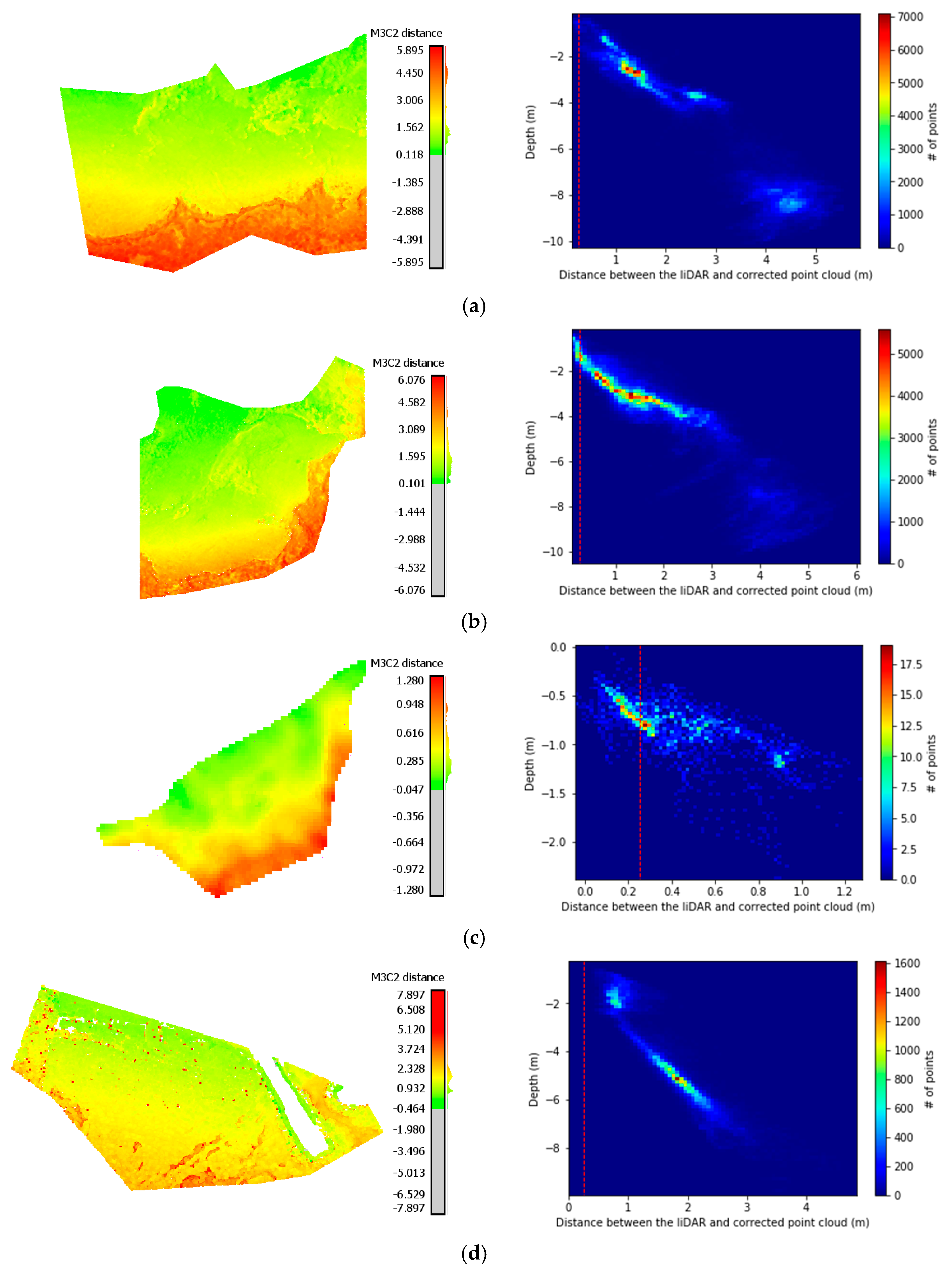
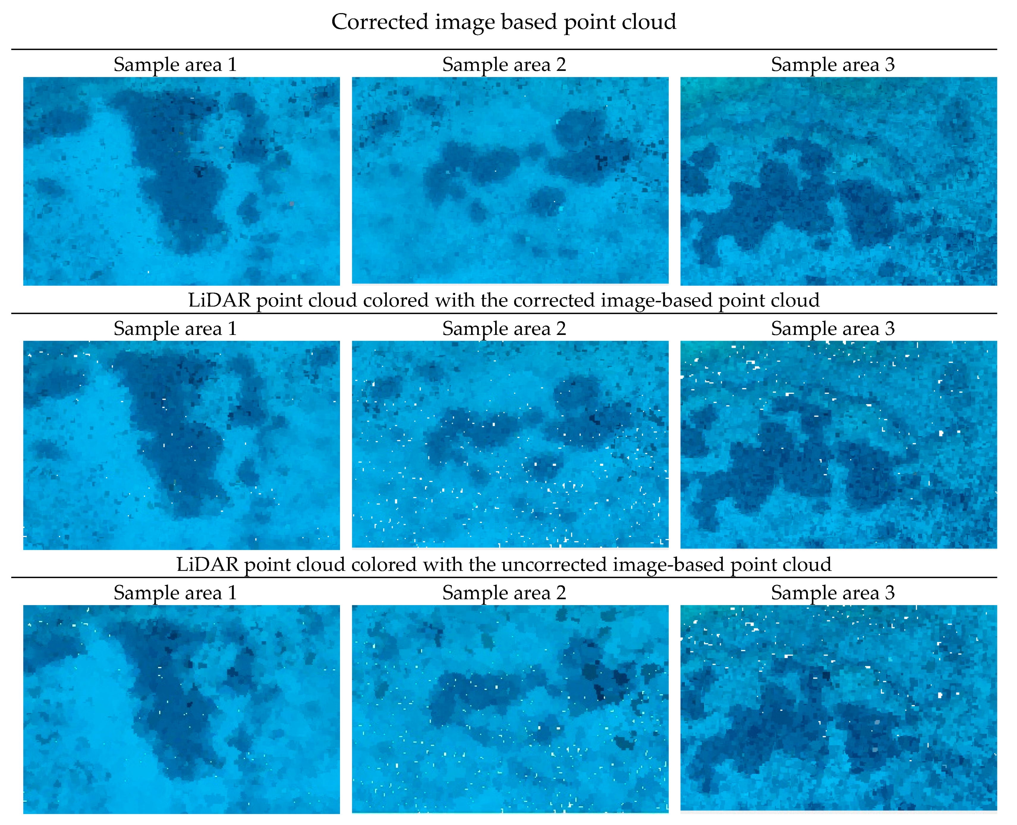
5.2.1. Comparing the Corrected Image-Based, and LiDAR Point Clouds

To evaluate the results of the proposed methodology, the initial point clouds of the SfM-MVS procedure and the point clouds resulting from the proposed methodology were compared with the LiDAR point clouds using the multiscale model to model cloud comparison (M3C2) [60] module in Cloud Compare freeware [61] to demonstrate the changes and the differences that are applied by the presented depth correction approach. The M3C2 algorithm offers accurate surface change measurement that is independent of point density [60]. In Figure 9, it can be observed that the distances between the reference data and the original image-based point clouds were increasing proportionally to the depth. These comparisons clarify that the refraction effect cannot be ignored in such applications.

In all four cases demonstrated in Figure 9, the Gaussian mean of the differences was significant. It reached 2.23 m (RMSE 2.64 m) in the Agia Napa test site [I] and [II] (Figure 9a,b), 0.44 m (RMSE 0.51 m) in the Amathouda test site (Figure 9c), and 1.38 m (RMSE 1.53 M) in the Dekelia test site (Figure 9d). Differences for the Dekelia (GPS) dataset are not demonstrated in Figure 9 due to the small number and the sparsity of points. The Gaussian mean of the differences in depths in this case reached 1.15 m. Since these values might be considered ‘negligible’ in some applications, it is important to stress that in the Amathouda test site, more than 30% of the compared image-based points presented a difference of 0.60–1.00 m from the LiDAR points; in Agia Napa, the same percentage presented differences of 3.00–6.07 m; i.e., 20%–41.1% percent of the real depth, while in Dekelia, the same percentage of points presented differences of 1.76–4.94 m. As can be observed in the right column of Figure 9, the majority of the points in all four areas are far from the red dashed lines representing the accuracy limits generally accepted for hydrography, as introduced by the International Hydrographic Organization (IHO) [76].

Figure 10 presents the histograms of the cloud to cloud distances (M3C2) between the LiDAR point cloud and the point clouds produced from the predicted model trained on each dataset in relation with the real depth. There, the dashed lines in red represent the accuracy limits generally accepted for hydrography as introduced by the International Hydrographic Organization (IHO) [76].

Table 3. The results of the comparisons between the predicted models for all tests performed.

Training Site	Training Points	Training Percentage (%)	Fitting Score	Evaluation Site	Max/Min Depth of Test Site	Evaluation Points	Corrected Data		Uncorrected Data
							Mean Dist. (m)	Stdev (m)	Mean Dist. (m)	Stdev (m)
Ag. Napa[I]	627.552	5	0.984	Ag. Napa[II]	14.7/0.30	661.208	−0.15	0.49	2.23	1.42
Ag. Napa[I]	627.552	30	0.984	Ag. Napa[II]	14.7/0.30	661.208	−0.14	0.50	2.23	1.42
Ag. Napa[I]	627.552	5	0.984	Amathouda	5.57/0.10	5400	−0.03	0.19	0.44	0.26
Ag. Napa[I]	627.552	30	0.984	Amathouda	5.57/0.10	5400	−0.03	0.19	0.44	0.26
Ag. Napa[I]	627.552	5	0.984	Dekelia	10.1/0.09	101.887	−0.12	0.25	1.72	0.76
Ag. Napa[I]	627.552	30	0.984	Dekelia	10.1/0.09	101.887	−0.12	0.25	1.72	0.76
Ag. Napa[I]	627.552	5	0.984	Dekelia (GPS)	7.0/0.30	208	−0.12	0.46	−1.15	0.55
Ag. Napa[I]	627.552	30	0.984	Dekelia (GPS)	7.0/0.30	208	−0.12	0.46	−1.15	0.55
Ag. Napa[II]	661.208	5	0.967	Ag. Napa[I]	14.8/0.20	627.552	0.14	0.49	2.23	1.42
Ag. Napa[II]	661.208	30	0.967	Ag. Napa[I]	14.8/0.20	627.552	0.14	0.49	2.23	1.42
Ag. Napa[II]	661.208	5	0.967	Amathouda	5.57/0.10	5400	0.25	0.11	0.44	0.26
Ag. Napa[II]	661.208	30	0.967	Amathouda	5.57/0.10	5400	0.25	0.11	0.44	0.26
Ag. Napa[II]	661.208	5	0.967	Dekelia	10.1/0.09	101.887	−0.23	0.28	1.72	0.76
Ag. Napa[II]	661.208	30	0.967	Dekelia	10.1/0.09	101.887	−0.22	0.28	1.72	0.76
Ag. Napa[II]	661.208	5	0.967	Dekelia (GPS)	7.0/0.30	208	−0.27	0.48	−1.15	0.55
Ag. Napa[II]	661.208	30	0.967	Dekelia (GPS)	7.0/0.30	208	−0.25	0.48	−1.15	0.55
Amathouda	5400	100	-	Ag. Napa[I]	14.8/0.20	627.552	−0.10	0.45	2.23	1.42
Amathouda	5400	100	-	Ag. Napa[II]	14.7/0.30	661.208	−0.26	0.49	2.23	1.42
Amathouda	5400	100	-	Dekelia	10.1/0.09	101.887	0.02	0.26	1.72	0.76
Amathouda	5400	100	-	Dekelia (GPS)	7.0/0.30	208	−0.02	0.46	−1.15	0.55
Merged	11873	100	-	Ag. Napa[I]	14.8/0.20	627.552	0.13	0.45	2.23	1.42
Merged	11873	100	-	Ag. Napa[II]	14.7/0.30	661.208	−0.06	0.50	2.23	1.42
Merged	11873	100	-	Amathouda	5.57/0.10	5400	0.00	0.18	0.44	0.26
Merged	11873	100	-	Dekelia	10.1/0.09	101.887	−0.19	0.24	1.72	0.76
Merged	11873	100	-	Dekelia(GPS)	7.0/0.30	208	−0.17	0.46	−1.15	0.55
Dekelia	101.887	100	-	Ag. Napa[I]	14.8/0.20	627.552	0.13	0.51	2.23	1.42
Dekelia	101.887	100	-	Ag. Napa[II]	14.7/0.30	661.208	−0.15	0.56	2.23	1.42
Dekelia	101.887	100	-	Amathouda	5.57/0.10	5400	−0.21	0.18	0.44	0.26
				Overall Average			−0.068	0.366	1.013	0.844
				Stdev			0.149	0.142	1.307	0.461

presents the results of each one of the 28 tests performed with every detail. Both in Figure 10 and Table 3, a great improvement is observed. More specifically, in Agia Napa [I] test site, the initial 2.23 m mean distance was reduced to −0.10 m; in Amathouda, the initial mean distance of 0.44 m was reduced to −0.03 m, while in Dekelia test site, the initial mean distance of 0.44 m was reduced to 0.00 m—by using the model trained on the Merged dataset, including outlier, points such as seagrass, that are not captured in the LiDAR point clouds for both cases or are caused due to point cloud noise again in areas with seagrass or poor texture. It is also important to note that the large distances between the clouds observed in Figure 9 disappeared. This improvement was observed in every test performed, proving that the proposed methodology based on machine learning achieves a great reduction of the errors caused by the refraction in the seabed point clouds.

5.2.2. Fitting Score

Another measure to evaluate the predicted model in cases where a percentage of the dataset has been used for training and the rest has been used for testing, is by computing the coefficient R² of each, which is the fitting score and is defined as

$$R^2=1-\frac{{\displaystyle \sum }{\left(Z_{true}-Z_{predicted}\right)}^2}{{\displaystyle \sum }{\left(Z_{true}-Z_{true.mean}\right)}^2}$$

(6)

The best possible score is 1.0 and it may also be negative [74]. Z_true is the real value of the depth of the points not used for training, while the Z_predicted is the predicted depth for these points, using the model trained on the rest of the points. The fitting score is calculated only in cases where a percentage of the dataset is used for training. Results in Table 3 highlight the robustness of the proposed depth correction framework.

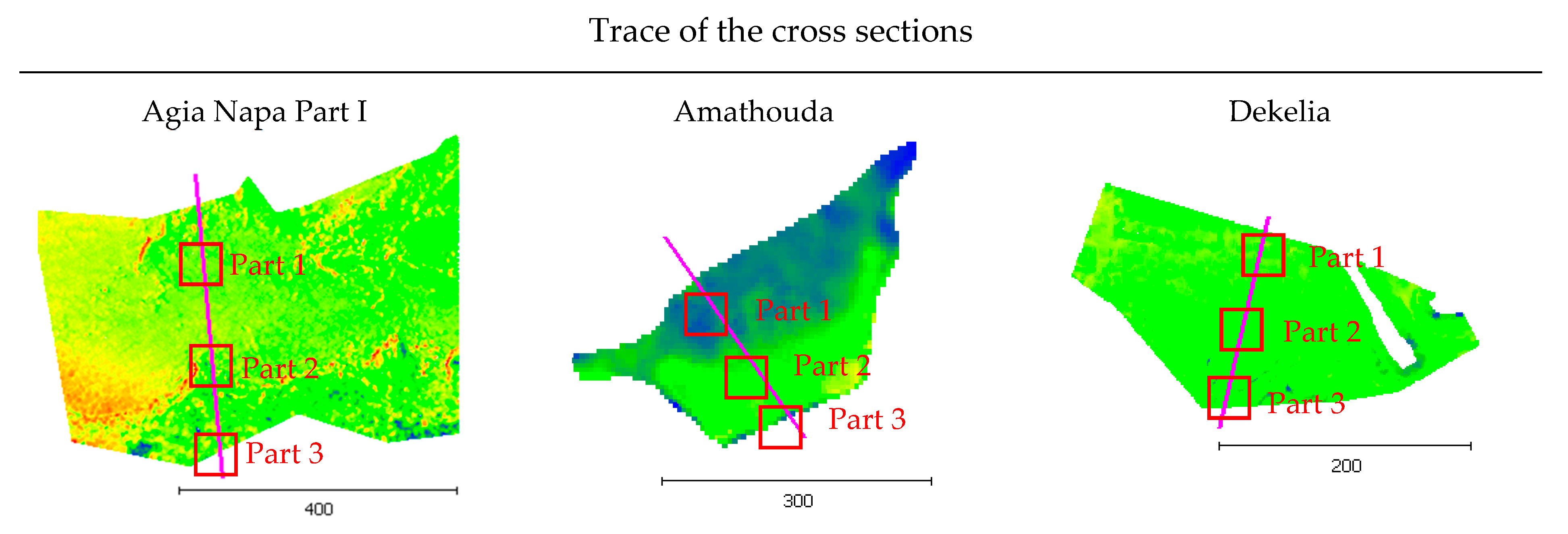
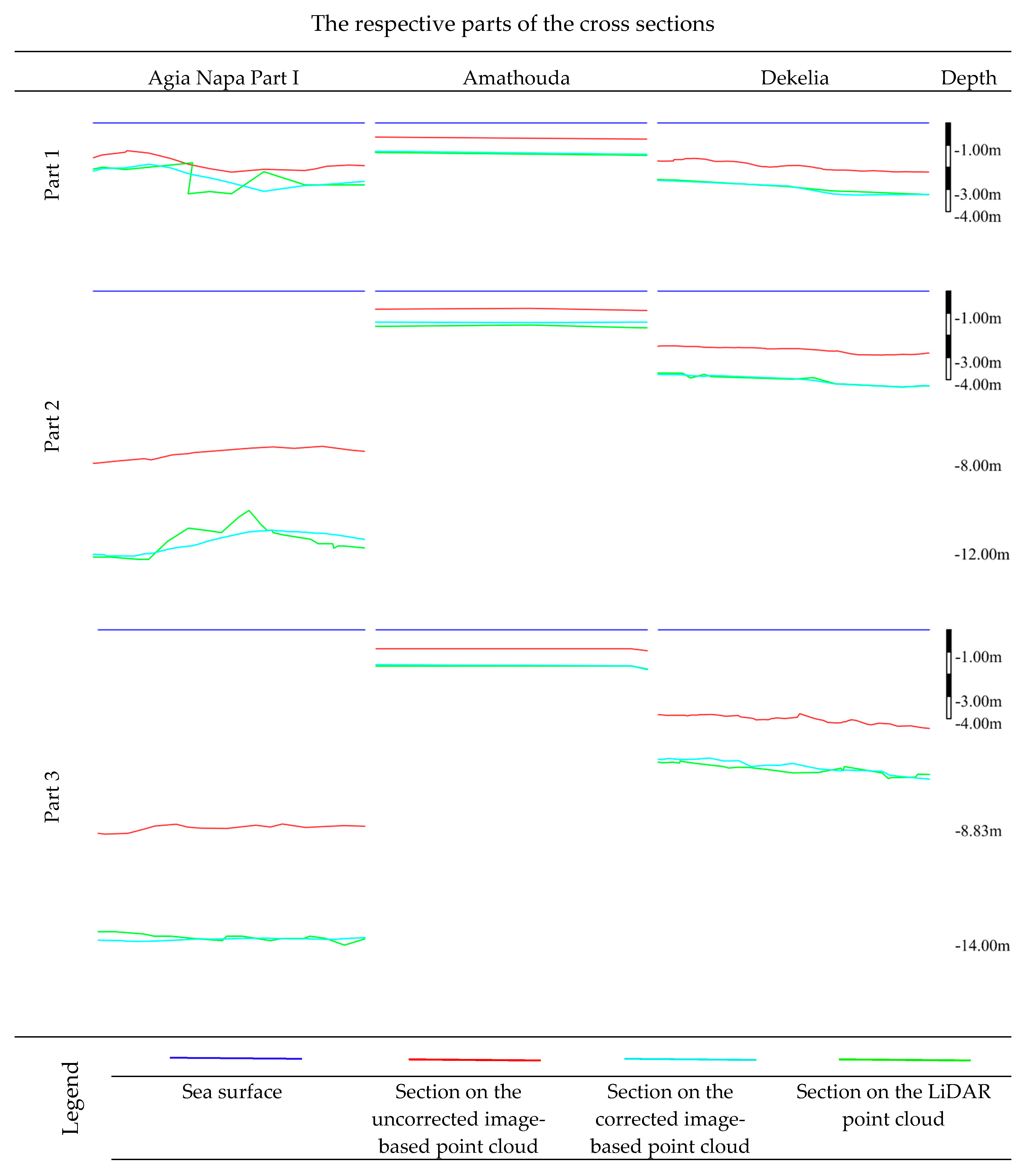
5.2.3. Seabed Cross Sections

Several differences observed between the image-based point clouds and the LiDAR data were not due to the proposed depth correction approach. Cross sections of the seabed were generated in order to prove the performance of the proposed method, excluding differences between the compared point clouds. In Figure 11 the footprints of the representative cross sections are demonstrated, together with three parts of the section (top, middle, and end).

In Figure 12 the blue line corresponds to the water surface, while the green one corresponds to the LiDAR data. The cyan line is the corrected depth after the application of the proposed approach, while the red line corresponds to the depths derived from the initial uncorrected image-based point cloud. The first row of the cross sections represents Part 1, the second Part 2, and the third Part 3.

These parts highlight the high performance of the algorithm and the differences between the point clouds, reported above. In more detail, in the first and the second part of the section presented, it can be noticed that even if the corrected image-based point cloud almost matches the LiDAR one on the left and the right side of the sections, in the middle parts, errors are introduced. These are mainly caused by gross errors, which however, are not related to the depth correction approach. However, in the third part of the section, it is obvious that even when the depth reaches 14 m, the corrected image-based point cloud matches the LiDAR one, indicating a very high performance of the proposed approach. Excluding these differences, the corrected image-based point cloud presents deviations of less than 0.05 m (0.36% remaining error at 14 m depth) from the LiDAR point cloud.

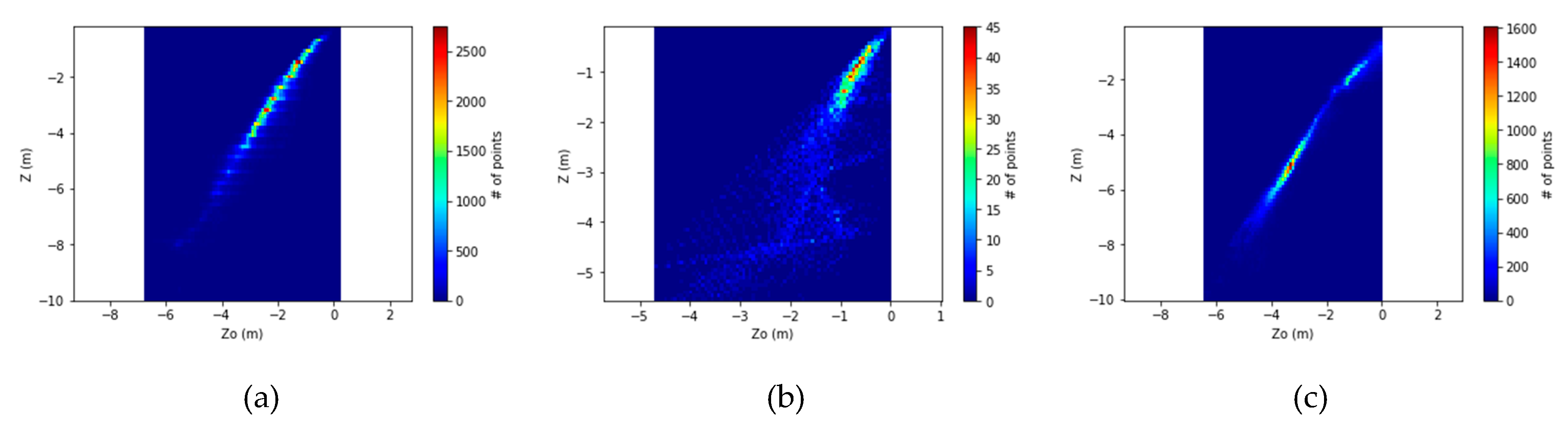
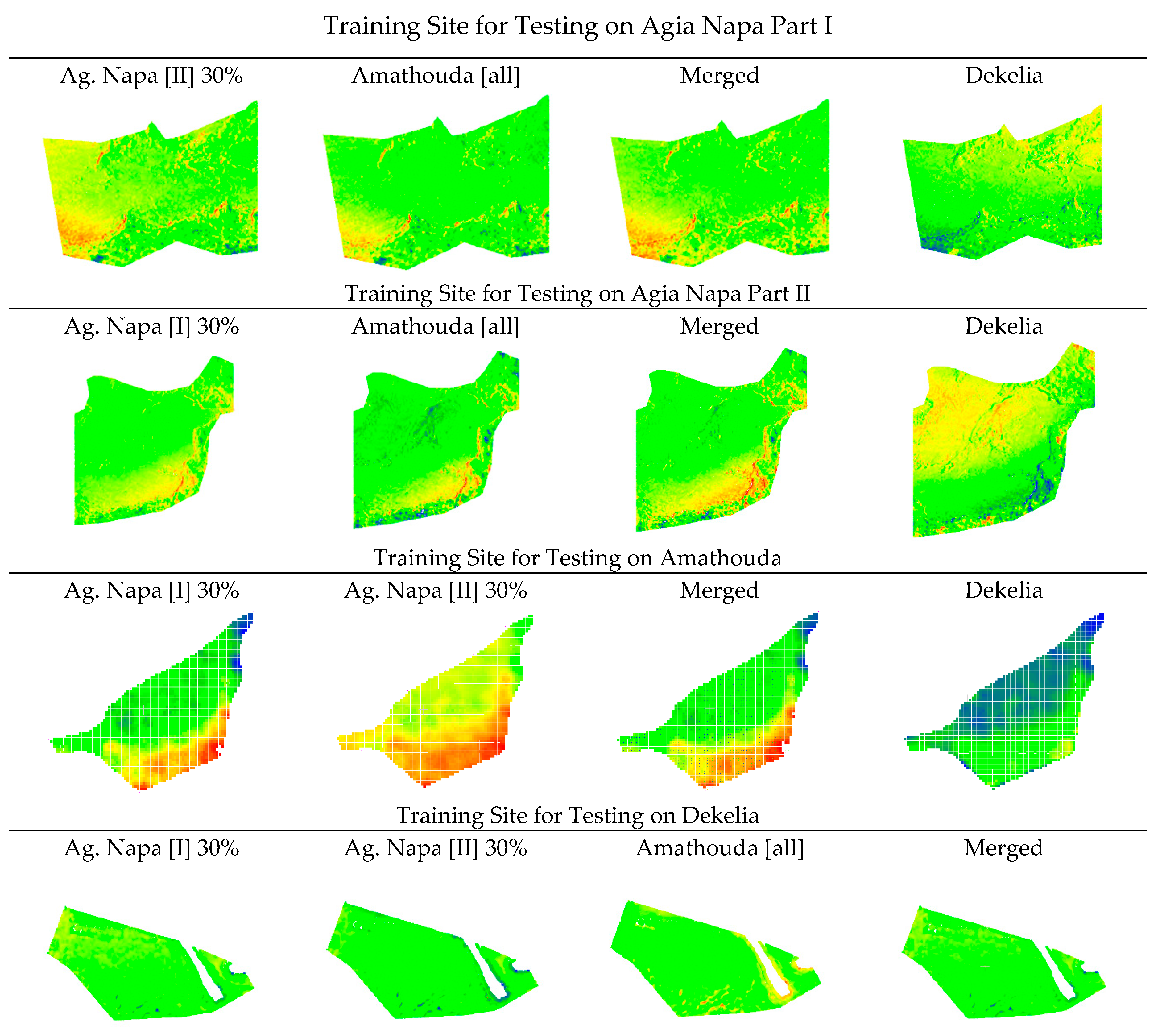
5.2.4. Distribution Patterns of Remaining Errors

The larger differences between the predicted and the LiDAR depths are observed in some specific areas, or areas with same characteristics, as may be observed in Figure 13. In more detail, the lower-left area of Agia Napa Part I test site and the lower-right area of Agia Napa Part II test site, had constantly larger errors than other areas of the same depth. This can be explained by their unfavorable position in the photogrammetric block, as these areas (i) are far from the control points, (ii) situated on the shore, and (iii) they lie in the periphery of the block. However, it is noticeable that these two areas presented smaller deviations from the LiDAR point cloud when the model was trained in Amathouda test site, a totally characteristically different and shallower test site. Additionally, areas with small rock formations also presented differences. This is attributed to the different level of detail in these areas between the LiDAR point cloud and the image-based one, since LiDAR’s average point spacing is about 1.1 m. These small rock formations in many cases led M3C2 to detect larger distances in those parts of the site and were responsible for the increased standard deviation of the M3C2 distances (Table 3). Regarding the Dekelia test site, larger differences were observed in the area around the removed breakwater, something that was expected due to its construction characteristics (Figure 2c), and due to the fact that in this area the sea is quite turbid.

6. Fusing the Corrected Image-Based, and LiDAR Point Clouds

To demonstrate the performance of the proposed approach and highlight possible exploitation of the results achieved, fusion of the LiDAR and the depth-corrected image-based point clouds was performed. The results are presented and evaluated with qualitative and quantitative methods. To that end, examples of color transferring from the image-based point cloud to the LiDAR point cloud are presented, together with hole filling actions in both point clouds. For this approach, the Agia Napa test area was used, since, due to its coverage and its depth, it presents many opportunities for demonstrating various results.

6.1. Color Transfer to LiDAR Data

As reported in Section 1.2, color information is crucial for a number of applications. A simple interpolation approach was followed to assign color values to the LiDAR point clouds. For every point of the LiDAR point cloud, the color value of the nearest neighbor in the corrected image-based point cloud was assigned. In Figure 14a, the corrected image-based point cloud is presented, while in Figure 14b, the non-colored LiDAR point cloud is shown. In Figure 14c, the resulting colored LiDAR point cloud of the Agia Napa test area is presented. As can be noticed, excluding areas of lower density on the LiDAR point cloud, where it is quite difficult to recognize the colors at this scale, the results are very satisfactory. Although the LiDAR point cloud is much less dense than the image-based one, colors are assigned to it in a very rigorous way, achieving high reliability in the spatial space and managing to deliver a LiDAR point cloud with high quality color information. Following this process and in order to prove the importance of using the corrected image-based point cloud for coloring LiDAR point clouds, instead of using the uncorrected one, a second color interpolation approach was performed using the uncorrected image-based cloud. The results on three sample areas of the seabed are presented in Figure 15.

The first two columns of Figure 15 depict an area of Agia Napa[I] dataset, while the third one depicts an area of Agia Napa (II) dataset. The first row of images in Figure 15 depicts the three sample areas on the image based point cloud; the second row of images demonstrate the same areas on the LiDAR point cloud colored with the corrected image-based point cloud; and the third row of images depict the three areas on the LiDAR point cloud colored with the uncorrected image-based one.

As can be easily noticed, the color of the seabed point clouds is almost identical in the first two rows, while certain areas in the third row present many differences, fluctuations, and noise. In more detail, by observing the total of the colored seabed point clouds, it was noticed that as the depth increases, colors are assigned in an incorrect way, something that was expected due to the large distance between the two point-clouds. This leads to an incorrect representation of the seabed at depths of more than 2 to 3 meters. As can be noticed in Figure 15, not only do the resultantly assigned colors create a more rough and unclear seabed, but seagrass and rocky areas are represented in a totally different shape and area, affecting future exploitation and processing of the point cloud datasets, such as for seabed classification, orthoimage generation, etc.

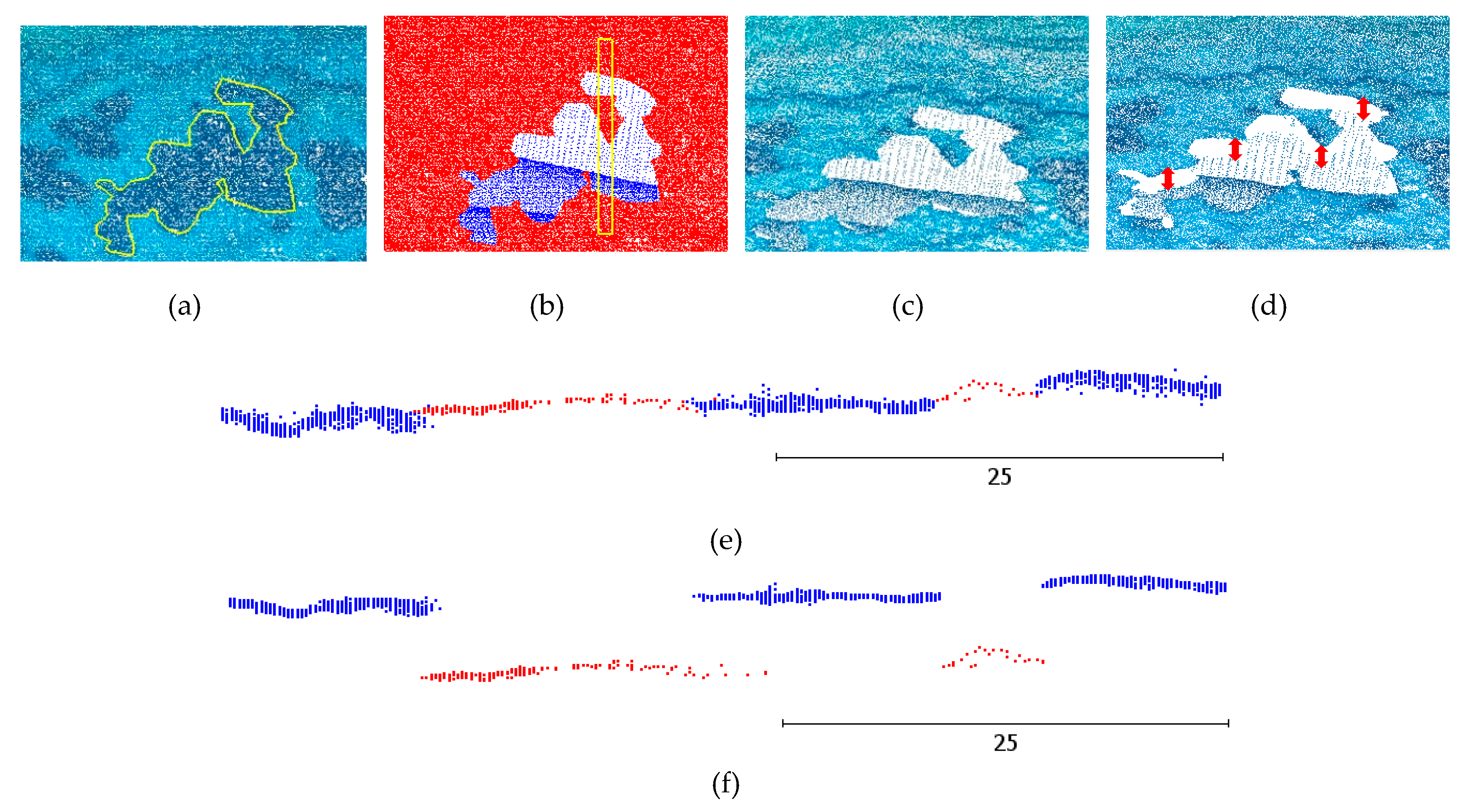
6.2. Seamless Hole Filling

Seamless hole filling of seabed areas was performed and demonstrated in the Agia Napa test area. To that end, an area of the corrected and the uncorrected image-based point cloud, covered with seagrass and lying at 11.70 m depth was deleted in order to create an artificial hole on the point cloud. Then, this area was filled with the respective LiDAR point cloud. In Figure 16a, the seagrass area, deleted to create the desirable hole, is depicted with the yellow polyline. In Figure 16b, the image-based point cloud is demonstrated with red, while the LiDAR points used for filling are shown in blue. The yellow rectangular describes the area of sections shown in Figure 16e,f. In Figure 16c, the hole in the corrected image-based point cloud is filled with the LiDAR data, while in Figure 16d, the hole in the uncorrected image-based point cloud is filled with the LiDAR data. In the first case of Figure 16c, it is obvious that the two point clouds are at the same depth and facilitate a seamless hole filling, even at the depth of 11.70 m. However, in Figure 16d, it is obvious that the depth difference of the two point clouds (highlighted with red arrows in Figure 16d) creates a huge obstacle in merging the two point clouds and having a seamless result. To further prove the above, cross sections were created of the area (in the yellow rectangle in Figure 16b).

In the two generated cross sections of the point clouds—demonstrated in Figure 16e for the corrected image based point cloud, and in Figure 16f for the uncorrected image based point cloud—the LiDAR point cloud is in red, while the image based one in blue. It is clear that the proposed algorithm corrects the image-based point cloud to a degree facilitating the merging and the fusion of the point clouds of the two different sources.

7. Discussion

The experiments performed demonstrated that the model has significant potential for generalization over different areas and in shallow waters, and it can be used when no LiDAR data are available. The approach proposed is independent from the UAV imaging system, the camera type, the flying height, the camera to water surface distance, and the base-to-height (B/H) ratio. Additional data, e.g., camera orientations and camera intrinsic parameters, for predicting the correct depth of a point cloud, are not required. This is a very important advantage of the proposed method compared to the current state-of-the-art methods that have been designed to address refraction errors in seabed mapping using aerial imagery.

The limitations of this method are mainly imposed by the SfM-MVS errors in areas having texture of low quality and non-static objects; e.g., sand and seagrass areas, respectively. Regarding training, slight limitations are also imposed due to incompatibilities between the LiDAR point cloud and the image-based one. Among others, the different level of detail imposed additional errors in the point cloud comparison and compromised the absolute accuracy of the method. Additionally, the unfavorable position of the GCPs in the photogrammetric block situated on the shore may also compromised the accuracy of the block and the point cloud, respectively, in the deeper areas of the seabed that are far from those. However, those issues do not affect the principle of the main goal of the presented approach, which is to systematically solve the depth underestimation problem, by predicting the correct depth.

To improve the accuracy of the predicted models, and thus the depth accuracy of the corrected point clouds, concurrently acquired images and ground truth data (i.e., bathymetric LiDAR data), having the same level of detail, should be available in order to avoid differences in the point clouds. Additionally, favorable conditions, such as clear water, calm water surface, and bottom texture are required, in order to improve the results of the SfM-MVS processing and eliminate the noise of the image-based point cloud generated.

The proposed approach can be used also in areas were LiDAR data of low density are available, in order to create a denser seabed representation. In particular, the data fusion procedure implemented demonstrated its high potential towards the efficient coloring of LiDAR point clouds, gap and hole filling, and surface seabed model updating, thus minimizing costs and time for many applications. This achievement is of high importance when it comes to multitemporal and multi-source monitoring of seabed areas, facilitating the update of specific parts of the seabed, as well as filling holes in point clouds generated by a source failing to produce reliable results in specific areas; i.e., areas with sun glint in aerial imagery, areas covered by ships or other floating objects in LiDAR, surveys, etc.

8. Conclusions

In the proposed approach, an SVR model was developed based on known depth observations from bathymetric LiDAR surveys, able to estimate with high accuracy, the real depths of point clouds derived from conventional SfM-MVS procedures using aerial imagery. Experimental results over three test areas in Cyprus (Agia Napa, Amathouda, and Dekelia) of different flying heights, different depths, and different seabed characteristics, along with the quantitative validation performed, indicated the high potential of the developed approach. Twenty-six out of twenty-eight different tests (Table 3), or 92.9% of the tests, proved that the proposed method meets and exceeds the accuracy standards generally accepted for hydrography, as introduced by the International Hydrographic Organization (IHO), where in its simplest form, the vertical accuracy requirement for shallow water hydrography can be set as a total of ±25cm (one sigma) from all sources, including tides [76]. If more accurate ground truth data were available, the results of the proposed approach would definitely be better.

References

1. Agrafiotis, P.; Skarlatos, D.; Forbes, T.; Poullis, C.; Skamantzari, M.; Georgopoulos, A. Underwater photogrammetry in very shallow waters: main challenges and caustics effect removal. Int. Arch. Photogramm. Remote Sens. Spat. Inf. Sci. 2018, XLII-2, 15–22. [Google Scholar] [CrossRef]
2. Karara, H.M. Non-Topographic Photogrammetry, 2nd ed.; American Society for Photogrammetry and Remote Sensing: Falls Church, VA, USA, 1989. [Google Scholar]
3. Menna, F.; Agrafiotis, P.; Georgopoulos, A. State of the art and applications in archaeological underwater 3D recording and mapping. J. Cult. Herit. 2018. [Google Scholar] [CrossRef]
4. Skarlatos, D.; Agrafiotis, P. A Novel Iterative Water Refraction Correction Algorithm for Use in Structure from Motion Photogrammetric Pipeline. J. Mar. Sci. Eng. 2018, 6, 77. [Google Scholar] [CrossRef]
5. Green, E.; Mumby, P.; Edwards, A.; Clark, C. Remote Sensing: Handbook for Tropical Coastal Management; United Nations Educational Scientific and Cultural Organization (UNESCO): London, UK, 2000. [Google Scholar]
6. Agrafiotis, P.; Skarlatos, D.; Georgopoulos, A.; Karantzalos, K. Shallow water bathymetry mapping from UAV imagery based on machine learning. Int. Arch. Photogramm. Remote Sens. Spat. Inf. Sci. 2019, XLII-2/W10, 9–16. [Google Scholar] [CrossRef]
7. Lavest, J.; Rives, G.; Lapresté, J. Underwater camera calibration. In Computer Vision—ECCV; Vernon, D., Ed.; Springer: Berlin, Germany, 2000; pp. 654–668. [Google Scholar]
8. Shortis, M. Camera Calibration Techniques for Accurate Measurement Underwater. In 3D Recording and Interpretation for Maritime Archaeology; Springer: Cham, Switzerland, 2019; pp. 11–27. [Google Scholar] [Green Version]
9. Elnashef, B.; Filin, S. Direct linear and refraction-invariant pose estimation and calibration model for underwater imaging. ISPRS J. Photogramm. Remote Sens. 2019, 154, 259–271. [Google Scholar] [CrossRef]
10. Fryer, J.G.; Kniest, H.T. Errors in Depth Determination Caused by Waves in Through-Water Photogrammetry. Photogramm. Rec. 1985, 11, 745–753. [Google Scholar] [CrossRef]
11. Okamoto, A. Wave influences in two-media photogrammetry. Photogramm. Eng. Remote Sens. 1982, 48, 1487–1499. [Google Scholar]
12. Agrafiotis, P.; Georgopoulos, A. Camera constant in the case of two media photogrammetry. Int. Arch. Photogramm. Remote Sens. Spat. Inf. Sci. 2015, XL-5/W5, 1–6. [Google Scholar] [CrossRef]
13. Georgopoulos, A.; Agrafiotis, P. Documentation of a submerged monument using improved two media techniques. In Proceedings of the 2012 18th International Conference on Virtual Systems and Multimedia, Milan, Italy, 2–5 September 2012; pp. 173–180. [Google Scholar] [CrossRef]
14. Maas, H.-G. On the Accuracy Potential in Underwater/Multimedia Photogrammetry. Sensors 2015, 15, 18140–18152. [Google Scholar] [CrossRef]
15. Allouis, T.; Bailly, J.S.; Pastol, Y.; Le Roux, C. Comparison of LiDAR waveform processing methods for very shallow water bathymetry using Raman, near-infrared and green signals. Earth Surf. Process. Landf. 2010, 5, 640–650. [Google Scholar] [CrossRef]
16. Schwarz, R.; Mandlburger, G.; Pfennigbauer, M.; Pfeifer, N. Design and evaluation of a full-wave surface and bottom-detection algorithm for LiDAR bathymetry of very shallow waters. ISPRS J. Photogramm. Remote Sens. 2019, 150, 1–10. [Google Scholar] [CrossRef]
17. van den Bergh, J.; Schutz, J.; Chirayath, V.; Li, A. A 3D Active Learning Application for NeMO-Net, the NASA Neural Multi-Modal Observation and Training Network for Global Coral Reef Assessment. In Proceedings of the AGU Fall Meeting, New Orleans, LA, USA, 11–15 December 2017. [Google Scholar]
18. Butler, J.B.; Lane, S.N.; Chandler, J.H.; Porfiri, E. Through-water close range digital photogrammetry in flume and field environments. Photogramm. Rec. 2002, 17, 419–439. [Google Scholar] [CrossRef]
19. Tewinkel, G.C. Water depths from aerial photographs. Photogramm. Eng. 1963, 29, 1037–1042. [Google Scholar]
20. Shmutter, B.; Bonfiglioli, L. Orientation problem in two-medium photogrammetry. Photogramm. Eng. 1967, 33, 1421–1428. [Google Scholar]
21. Wang, Z. Principles of Photogrammetry (with Remote Sensing); Publishing House of Surveying and Mapping: Beijing, China, 1990. [Google Scholar]
22. Shan, J. Relative orientation for two-media photogrammetry. Photogramm. Rec. 1994, 14, 993–999. [Google Scholar] [CrossRef]
23. Fryer, J.F. Photogrammetry through shallow waters. Aust. J. Geod. Photogramm. Surv. 1983, 38, 25–38. [Google Scholar]
24. Whittlesey, J.H. Elevated and airborne photogrammetry and stereo photography. In Photography in Archaeological Research; Harp, E., Jr., Ed.; University of New Mexico Press: Albuquerque, NM, USA, 1975; pp. 223–259. [Google Scholar]
25. Westaway, R.; Lane, S.; Hicks, M. Remote sensing of clear-water, shallow, gravel-bed rivers using digital photogrammetry. Photogramm. Eng. Remote Sens. 2010, 67, 1271–1281. [Google Scholar]
26. Elfick, M.H.; Fryer, J.G. Mapping in shallow water. Int. Arch. Photogramm. Remote Sens. 1984, 25, 240–247. [Google Scholar]
27. Partama, I.G.Y.; Kanno, A.; Ueda, M.; Akamatsu, Y.; Inui, R.; Sekine, M.; Yamamoto, K.; Imai, T.; Higuchi, T. Removal of water-surface reflection effects with a temporal minimum filter for UAV-based shallow-water photogrammetry. Earth Surf. Process. Landf. 2018, 43, 2673–2682. [Google Scholar] [CrossRef]
28. Ferreira, R.; Costeira, J.P.; Silvestre, C.; Sousa, I.; Santos, J.A. Using stereo image reconstruction to survey scale models of rubble-mound structures. In Proceedings of the First International Conference on the Application of Physical Modelling to Port and Coastal Protection, Porto, Portugal, 22–26 May 2006. [Google Scholar]
29. Muslow, C. A flexible multi-media bundle approach. Int. Arch. Photogramm. Remote Sens. Spat. Inf. Sci. 2010, XXXVIII, 472–477. [Google Scholar]
30. Wolff, K.; Forstner, W. Exploiting the multi view geometry for automatic surfaces reconstruction using feature based matching in multi media photogrammetry. Int. Arch. Photogramm. Remote Sens. Spat. Inf. Sci. 2000, XXXIII Pt B5, 900–907. [Google Scholar]
31. Ke, X.; Sutton, M.A.; Lessner, S.M.; Yost, M. Robust stereo vision and calibration methodology for accurate three-dimensional digital image correlation measurements on submerged objects. J. Strain Anal. Eng. Des. 2008, 43, 689–704. [Google Scholar] [CrossRef]
32. Byrne, P.M.; Honey, F.R. Air survey and satellite imagery tools for shallow water bathymetry. In Proceedings of the 20th Australian Survey Congress, Shrewsbury, UK, 20 May 1977; pp. 103–119. [Google Scholar]
33. Harris, W.D.; Umbach, M.J. Underwater mapping. Photogramm. Eng. 1972, 38, 765. [Google Scholar]
34. Masry, S.E. Measurement of water depth by the analytical plotter. Int. Hydrogr. Rev. 1975, 52, 75–86. [Google Scholar]
35. Dietrich, J.T. Bathymetric Structure-from-Motion: Extracting shallow stream bathymetry from multi-view stereo photogrammetry. Earth Surf. Process. Landf. 2017, 42, 355–364. [Google Scholar] [CrossRef]
36. Telem, G.; Filin, S. Photogrammetric modeling of underwater environments. ISPRS J. Photogramm. Remote Sens. 2010, 65, 433–444. [Google Scholar] [CrossRef]
37. Woodget, A.S.; Carbonneau, P.E.; Visser, F.; Maddock, I.P. Quantifying submerged fluvial topography using hyperspatial resolution UAS imagery and structure from motion photogrammetry. Earth Surf. Process. Landf. 2015, 40, 47–64. [Google Scholar] [CrossRef]
38. Murase, T.; Tanaka, M.; Tani, T.; Miyashita, Y.; Ohkawa, N.; Ishiguro, S.; Suzuki, Y.; Kayanne, H.; Yamano, H. A photogrammetric correction procedure for light refraction effects at a two-medium boundary. Photogramm. Eng. Remote Sens. 2008, 74, 1129–1136. [Google Scholar] [CrossRef]
39. Hodúl, M.; Bird, S.; Knudby, A.; Chénier, R. Satellite derived photogrammetric bathymetry. ISPRS J. Photogramm. Remote Sens. 2018, 142, 268–277. [Google Scholar] [CrossRef]
40. Qian, Y.; Zheng, Y.; Gong, M.; Yang, Y.H. Simultaneous 3D Reconstruction for Water Surface and Underwater Scene. In Proceedings of the European Conference on Computer Vision (ECCV), Munich, Germany, 8–14 September 2018; pp. 754–770. [Google Scholar]
41. Kasvi, E.; Salmela, J.; Lotsari, E.; Kumpula, T.; Lane, S.N. Comparison of remote sensing based approaches for mapping bathymetry of shallow, clear water rivers. Geomorphology 2019, 333, 180–197. [Google Scholar] [CrossRef]
42. Mandlburger, G. A case study on through-water dense image matching. Int. Arch. Photogramm. Remote Sens. Spatial Inf. Sci. 2018, XLII-2, 659–666. [Google Scholar] [CrossRef]
43. Mandlburger, G. Through-Water Dense Image Matching for Shallow Water Bathymetry. Photogramm. Eng. Remote Sens. 2019, 85, 445–455. [Google Scholar] [CrossRef]
44. Wimmer, M. Comparison of Active and Passive Optical Methods for Mapping River Bathymetry. Master’s Thesis, Vienna University of Technology, Vienna, Austria, 2016. [Google Scholar]
45. Wang, L.; Liu, H.; Su, H.; Wang, J. Bathymetry retrieval from optical images with spatially distributed support vector machines. GIScience Remote Sens. 2018, 1–15. [Google Scholar] [CrossRef]
46. Misra, A.; Vojinovic, Z.; Ramakrishnan, B.; Luijendijk, A.; Ranasinghe, R. Shallow water bathymetry mapping using Support Vector Machine (SVM) technique and multispectral imagery. Int. J. Remote Sens. 2018, 1–20. [Google Scholar] [CrossRef]
47. Mohamed, H.; Negm, A.; Zahran, M.; Saavedra, O.C. Bathymetry determination from high resolution satellite imagery using ensemble learning algorithms in Shallow Lakes: Case study El-Burullus Lake. Int. J. Environ. Sci. Dev. 2016, 7, 295. [Google Scholar] [CrossRef]
48. Traganos, D.; Poursanidis, D.; Aggarwal, B.; Chrysoulakis, N.; Reinartz, P. Estimating satellite-derived bathymetry (SDB) with the google earth engine and sentinel-2. Remote Sens. 2018, 10, 859. [Google Scholar] [CrossRef]
49. Niroumand-Jadidi, M.; Pahlevan, N.; Vitti, A. Mapping Substrate Types and Compositions in Shallow Streams. Remote Sens. 2019, 11, 262. [Google Scholar] [CrossRef]
50. Shintani, C.; Fonstad, M.A. Comparing remote-sensing techniques collecting bathymetric data from a gravel-bed river. Int. J. Remote Sens. 2017, 38, 2883–2902. [Google Scholar] [CrossRef]
51. Caballero, I.; Stumpf, R.P.; Meredith, A. Preliminary Assessment of Turbidity and Chlorophyll Impact on Bathymetry Derived from Sentinel-2A and Sentinel-3A Satellites in South Florida. Remote Sens. 2019, 11, 645. [Google Scholar] [CrossRef]
52. Legleiter, C.J.; Fosness, R.L. Defining the Limits of Spectrally Based Bathymetric Mapping on a Large River. Remote Sens. 2019, 11, 665. [Google Scholar] [CrossRef]
53. Cabezas, R.; Freifeld, O.; Rosman, G.; Fisher, J.W. Aerial reconstructions via probabilistic data fusion. In Proceedings of the IEEE Conference on Computer Vision and Pattern Recognition, Columbus, OH, USA, 24–27 June 2014; pp. 4010–4017. [Google Scholar]
54. Alvarez, L.; Moreno, H.; Segales, A.; Pham, T.; Pillar-Little, E.; Chilson, P. Merging unmanned aerial systems (UAS) imagery and echo soundings with an adaptive sampling technique for bathymetric surveys. Remote Sens. 2018, 10, 1362. [Google Scholar] [CrossRef]
55. Legleiter, C.J. Remote measurement of river morphology via fusion of LiDAR topography and spectrally based bathymetry. Earth Surf. Process. Landf. 2012, 37, 499–518. [Google Scholar] [CrossRef]
56. Coleman, J.B.; Yao, X.; Jordan, T.R.; Madden, M. Holes in the ocean: Filling voids in bathymetric lidar data. Comput. Geosci. 2011, 37, 474–484. [Google Scholar] [CrossRef]
57. Cheng, L.; Ma, L.; Cai, W.; Tong, L.; Li, M.; Du, P. Integration of Hyperspectral Imagery and Sparse Sonar Data for Shallow Water Bathymetry Mapping. IEEE Trans. Geosci. Remote Sens. 2015, 53, 3235–3249. [Google Scholar] [CrossRef]
58. Leon, J.X.; Phinn, S.R.; Hamylton, S.; Saunders, M.I. Filling the ‘white ribbon’—A multisource seamless digital elevation model for Lizard Island, northern Great Barrier Reef. Int. J. Remote Sens. 2013, 34, 6337–6354. [Google Scholar] [CrossRef]
59. Hasegawa, H.; Matsuo, K.; Koarai, M.; Watanabe, N.; Masaharu, H.; Fukushima, Y. DEM accuracy and the base to height (B/H) ratio of stereo images. Int. Arch. Photogramm. Remote Sens. 2000, 33, 356–359. [Google Scholar]
60. Lague, D.; Brodu, N.; Leroux, J. Accurate 3D comparison of complex topography with terrestrial laser scanner: Application to the Rangitikei canyon (NZ). ISPRS J. Photogramm. Remote Sens. 2013, 82, 10–26. [Google Scholar] [CrossRef]
61. CloudCompare (Version 2.11 Alpha) [GPL Software]. Available online: http://www.cloudcompare.org/ (accessed on 15 July 2019).
62. Remondino, F.; Spera, M.G.; Nocerino, E.; Menna, F.; Nex, F.; Gonizzi-Barsanti, S. Dense image matching: Comparisons and analyses. In Proceedings of the 2013 IEEE Digital Heritage International Congress (DigitalHeritage), Marseille, France, 28 October–1 November 2013; Volume 1, pp. 47–54. [Google Scholar]
63. Matthies, L.; Kanade, T.; Szeliski, R. Kalman filter-based algorithms for estimating depth from image sequences. Int. J. Comput. Vis. 1989, 3, 209–238. [Google Scholar] [CrossRef] [Green Version]
64. Okutomi, M.; Kanade, T. A multiple-baseline stereo. IEEE Trans. Pattern Anal. Mach. Intell. 1993, 15, 353–363. [Google Scholar] [CrossRef]
65. Ylimäki, M.; Heikkilä, J.; Kannala, J. Accurate 3-D Reconstruction with RGB-D Cameras using Depth Map Fusion and Pose Refinement. In Proceedings of the 2018 24th IEEE International Conference on Pattern Recognition (ICPR), Beijing, China, 20–24 August 2018; pp. 1977–1982. [Google Scholar]
66. Mangeruga, M.; Bruno, F.; Cozza, M.; Agrafiotis, P.; Skarlatos, D. Guidelines for Underwater Image Enhancement Based on Benchmarking of Different Methods. Remote Sens. 2018, 10, 1652. [Google Scholar] [CrossRef]
67. Leica HawkEye III. Available online: https://leica-geosystems.com/-/media/files/leicageosystems/products/datasheets/leica_hawkeye_iii_ds.ashx?la=en (accessed on 7 August 2019).
68. Skinner, K.D. Evaluation of LiDAR-Acquired Bathymetric and Topographic Data Accuracy in Various Hydrogeomorphic Settings in the Deadwood and South Fork Boise Rivers, West-Central Idaho 2007; U.S. Geological Survey: Reston, VA, USA, 2011. [Google Scholar]
69. Bailly, J.S.; Le Coarer, Y.; Languille, P.; Stigermark, C.J.; Allouis, T. Geostatistical estimations of bathymetric LiDAR errors on rivers. Earth Surf. Process. Landf. 2010, 35, 1199–1210. [Google Scholar] [CrossRef]
70. Fernandez-Diaz, J.C.; Glennie, C.L.; Carter, W.E.; Shrestha, R.L.; Sartori, M.P.; Singhania, A.; Legleiter, C.J.; Overstreet, B.T. Early results of simultaneous terrain and shallow water bathymetry mapping using a single-wavelength airborne LiDAR sensor. IEEE J. Sel. Top. Appl. Earth Obs. Remote Sens. 2014, 7, 623–635. [Google Scholar] [CrossRef]
71. Westfeld, P.; Maas, H.G.; Richter, K.; Weiß, R. Analysis and correction of ocean wave pattern induced systematic coordinate errors in airborne LiDAR bathymetry. ISPRS J. Photogramm. Remote Sens. 2017, 128, 314–325. [Google Scholar] [CrossRef]
72. Smola, A.J. Regression Estimation with Support Vector Learning Machines. Ph.D. Thesis, Technische Universität München, Munich, Germany, 1996. [Google Scholar]
73. Bishop, C.M. Pattern Recognition and Machine Learning; Springer: Berlin/Heidelberg, Germany, 2006. [Google Scholar]
74. Pedregosa, F.; Varoquaux, G.; Gramfort, A.; Michel, V.; Thirion, B.; Grisel, O.; Blondel, M.; Prettenhofer, P.; Weiss, R.; Dubourg, V.; et al. Scikit-learn: Machine learning in Python. J. Mach. Learn. Res. 2011, 12, 2825–2830. [Google Scholar]
75. Bergstra, J.; Bengio, Y. Random search for hyper-parameter optimization. J. Mach. Learn. Res. 2012, 13, 281–305. [Google Scholar]
76. Guenther, G.C.; Cunningham, A.G.; LaRocque, P.E.; Reid, D.J. Meeting the Accuracy Challenge in Airborne Bathymetry; National Oceanic Atmospheric Administration/NESDIS: Silver Spring, MD, USA, 2000. [Google Scholar]
Figure 1. The geometry of two-media photogrammetry for the multiple view case, retrieved from [6].
Remotesensing 11 02225 g001
Figure 2. The three validation test sites: (a) Agia Napa, (b) Amathouda, and (c) Dekelia. The areas with blue were used for the training and validating procedures. Distances are in meters.
Remotesensing 11 02225 g002
Figure 3. The selected images for the alternated base-to-height (B/H) ratio and the compared LiDAR point clouds using the multiscale model to model cloud comparison (M3C2) for (a) Agia Napa and (b) Amathouda. M3C2 distance is in (m).
Remotesensing 11 02225 g003
Figure 4. (a): Part I (left) and Part II (right) datasets from the Agia Napa test site in blue, the Amathouda test site in orange, and the Dekelia test site in magenta, all having the same scale (b): The distribution of the Z and Z0 values for each dataset.
Remotesensing 11 02225 g004
Figure 5. The established correlations based on a simple linear regression and SVM linear regression models, trained on Amathouda and Agia Napa datasets.
Remotesensing 11 02225 g005
Figure 6. The depth to apparent depth (Z–Z0) distribution of the used datasets: the Agia Napa Part I dataset over the full Agia Napa dataset (a). The Agia Napa Part II dataset over the full Agia Napa dataset and (b) the Amathouda dataset (c); the merged dataset over the Agia Napa and Amathouda datasets (d) and the Dekelia dataset; and (e) the Dekelia dataset over the full Agia Napa dataset (f).
Remotesensing 11 02225 g006
Figure 7. The Z–Z0 distribution of the employed datasets and their respective, predicted linear models.
Remotesensing 11 02225 g007
Figure 8. The Z–Z0 distribution of the employed datasets and the respective point densities: The histograms for Agia Napa (a), for Amathouda (b), and for Dekelia (c) test areas are presented.
Remotesensing 11 02225 g008
Figure 9. The initial M3C2 distances between the (reference) LiDAR point cloud and the uncorrected image-based point clouds derived from the SfM-MVS; (a) presents the M3C2 distances of Agia Napa (I); (b) presents the M3C2 distances of Agia Napa (II); (c) presents the M3C2 distances for Amathouda test site, and (d) presents the M3C2 distances Dekelia test site. The dashed lines in red represent the accuracy limits generally accepted for hydrography as introduced by the International Hydrographic Organization (IHO) [76]. M3C2 distances are in (m).
Remotesensing 11 02225 g009
Figure 10. The histograms of the M3C2 distances between the LiDAR point cloud and the corrected point clouds after the application of the proposed approach in relation to the real depth. The red dashed lines represent the accuracy limits generally accepted for hydrography, as introduced by the International Hydrographic Organization (IHO) [76].
Remotesensing 11 02225 g010
Figure 11. The footprints of the representative cross sections.
Remotesensing 11 02225 g011
Figure 12. Indicative parts of the cross-sections (X and Y axes have the same scale) from the Agia Napa (Part I) region after the application of the proposed approach when trained with 30% from the Part II region (first column); the Amathouda test site was predicted with the model trained on Dekelia (middle column); and the Dekelia test site with the model trained on Merged dataset (right column).
Remotesensing 11 02225 g012
Figure 13. The cloud to cloud (M3C2) distances between the LiDAR point cloud and the corrected point clouds after the implementation of the proposed approach, demonstrating the spatial patterns of the remaining errors.
Remotesensing 11 02225 g013
Figure 14. (a) The corrected image-based point cloud; (b) the non-colored LiDAR point cloud; and (c) the colored LiDAR point cloud based on (a).
Remotesensing 11 02225 g014
Figure 15. Three different sample areas of the Agia Napa seabed with depths between 9.95 m to 11.75 m. The first two columns depict two sample areas of the Agia Napa (I) seabed, while the third depicts a sample area of the Agia Napa (II) seabed. The first row depicts the three areas on the image-based point cloud; the second row, image on the LiDAR point cloud colored with the corrected image-based point cloud; and the third row depicts the three areas on the LiDAR point cloud, colored using the uncorrected image-based one. Point size is multiplied by a factor of four in order to facilitate visual comparisons.
Remotesensing 11 02225 g015
Figure 16. An example of the seamless hole filling area and indicative results.
Remotesensing 11 02225 g016