A High-Resolution Airborne Color-Infrared Camera Water Mask for the NASA ABoVE Campaign

Abstract

The airborne AirSWOT instrument suite, consisting of an interferometric Ka-band synthetic aperture radar and color-infrared (CIR) camera, was deployed to northern North America in July and August 2017 as part of the NASA Arctic-Boreal Vulnerability Experiment (ABoVE). We present validated, open (i.e., vegetation-free) surface water masks produced from high-resolution (1 m), co-registered AirSWOT CIR imagery using a semi-automated, object-based water classification. The imagery and resulting high-resolution water masks are available as open-access datasets and support interpretation of AirSWOT radar and other coincident ABoVE image products, including LVIS, UAVSAR, AIRMOSS, AVIRIS-NG, and CFIS. These synergies offer promising potential for multi-sensor analysis of Arctic-Boreal surface water bodies. In total, 3167 km² of open surface water were mapped from 23,380 km² of flight lines spanning 23 degrees of latitude and broad environmental gradients. Detected water body sizes range from 0.00004 km² (40 m²) to 15 km². Power-law extrapolations are commonly used to estimate the abundance of small lakes from coarser resolution imagery, and our mapped water bodies followed power-law distributions, but only for water bodies greater than 0.34 (±0.13) km² in area. For water bodies exceeding this size threshold, the coefficients of power-law fits vary for different Arctic-Boreal physiographic terrains (wetland, prairie pothole, lowland river valley, thermokarst, and Canadian Shield). Thus, direct mapping using high-resolution imagery remains the most accurate way to estimate the abundance of small surface water bodies. We conclude that empirical scaling relationships, useful for estimating total trace gas exchange and aquatic habitats on Arctic-Boreal landscapes, are uniquely enabled by high-resolution AirSWOT-like mappings and automated detection methods such as those developed here.

1. Introduction

Accurate mapping of terrestrial surface water bodies is necessary for understanding the hydrologic cycle, energy and biogeochemical cycles, aquatic habitats, and improving earth system models [1]. Spatially, the world’s greatest density of surface water bodies is in the Arctic-Boreal regions, and these water bodies change in extent based on climate variability and permafrost presence [2,3,4,5]. Current water maps are derived from lake censuses [6,7] and satellite remote sensing [8,9,10]. Large-scale satellite-based studies typically produce datasets with 30 m resolution, which limit the observable lakes to 0.002 km² (2000 m²) or larger [6,8]. Increasingly, the surface water area distribution has been shown to be a dynamic variable, and some satellite products contain multi-temporal information at both coarse global [11] and detailed regional scales [12]. As it stands, there is no one surface water map suitable for all spatial and temporal scales, and regional maps remain crucial for detailed hydrologic studies.

Regional studies have used high-resolution remote sensing data (<6 m resolution) and ground-based methods to map lakes as small as 0.0001 km² (100 m²) [13,14,15]. However, broad-scale mappings of water bodies <0.001 km² are limited and often focused on constructed farm ponds in temperate climates [14,16,17]. This limitation impedes scientific understanding of freshwater resources for at least three reasons: (1) the total count of small (<0.001 km²) water bodies is known to be large but remains highly uncertain, especially in Arctic-Boreal regions [8], (2) lakes, ponds and wetlands are often a net source of greenhouse gases, and their extent is used as inputs to climate models, although it is uncertain [18,19,20], and (3) these water bodies are important for ecosystem services such as nutrient processing and biodiversity [13,21,22].

In the absence of global, high-resolution maps, area scaling is often applied to estimate the abundance of small water bodies and, subsequently, total surface water area [8,23,24]. Especially at high resolution, it is hard to define a water body, as they are often ephemeral and can merge and sub-divide as water tables rise and fall [15]. A power-law scaling relationship (Equation (1)) has frequently been invoked to extrapolate lake areas for unmapped lakes [7,16,20,23,25,26], although the scale over which power-laws can be used is unclear. The form of the power-law equation is:

$$P\left(A\right)=C{A}^{-\alpha }$$

(1)

where A is water body area, P(A) is exceedance probability, the number of water bodies with area > A, and C and α are empirically-derived fitting coefficients. For example, Downing et al. [23] used a Pareto distribution, a form of a power-law with a horizontal shift, to model global lake areas larger than 0.1 km². More recent studies, using higher-resolution data, found that other distributions may be better suited to modeling small lakes [13,24] and that there is no regionally-consistent distribution [14,15]. Extrapolating with a lognormal distribution, for example, would imply 10–100 times fewer lakes, decreasing the global surface area and the number of small water bodies [24]. New, Landsat-based observations of global river area, which exhibits similar area-abundance relationships, are between 15% and 59% greater than scaling-based estimates [25,27,28]. Thus, while models of lake area distributions derived from coarse-resolution data may appear scale-invariant, including smaller water bodies demonstrates the contrary. This difference underscores the need for high-resolution surface water and wetland mapping.

To that end, we have produced a conservative, high-resolution map of open water bodies greater than 40 m² using airborne imagery. Data were collected from a color-infrared (CIR) camera included in the AirSWOT Ka-band radar instrument suite, designed to measure water surface elevation (WSE). These flights were part of the 2017 NASA Arctic-Boreal Vulnerability Experiment (ABoVE) campaign, which aims to quantify the vulnerability and resilience of North American arctic ecosystems and society, focusing on surface water, permafrost, carbon and disturbance [29]. There are existing surface water maps covering the ABoVE spatial domain derived from satellite observations, but they are much coarser (30–5000 m² pixel size) than airborne data [30,31]. The only broad-scale study of lake distribution at high resolution (<6 m pixel size) covers 923 km² [14,32] with limited coverage of the ABoVE domain. Our product was acquired over 23,380 km² of Arctic-Boreal land and water, including ground areas imaged within days or weeks of other ABoVE airborne sensors. Its broad extent and high spatial resolution produce a unique water map for the ongoing ABoVE campaign and allow us to test the effects of physiography on the water body distribution.

Here, we present a semi-automated workflow to classify open water area from CIR digital imagery and assess lake scaling statistics across the ABoVE domain in northern Canada and Alaska. In the following sections, we outline the 2017 ABoVE flight campaign, discuss AirSWOT camera data acquisition and processing, develop an open water classification workflow, show how high-resolution CIR imagery can enhance data interpretation from other ABoVE flight campaigns, use the derived water body product to test the hypothesis that lake-area scaling can be described by a power-law distribution, and show how power-law fitting parameters (if applicable) vary across physiographic terrains.

2. Materials and Methods

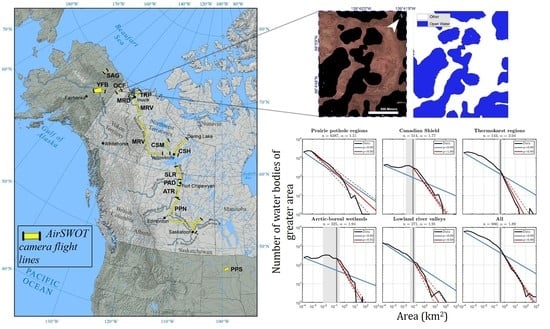
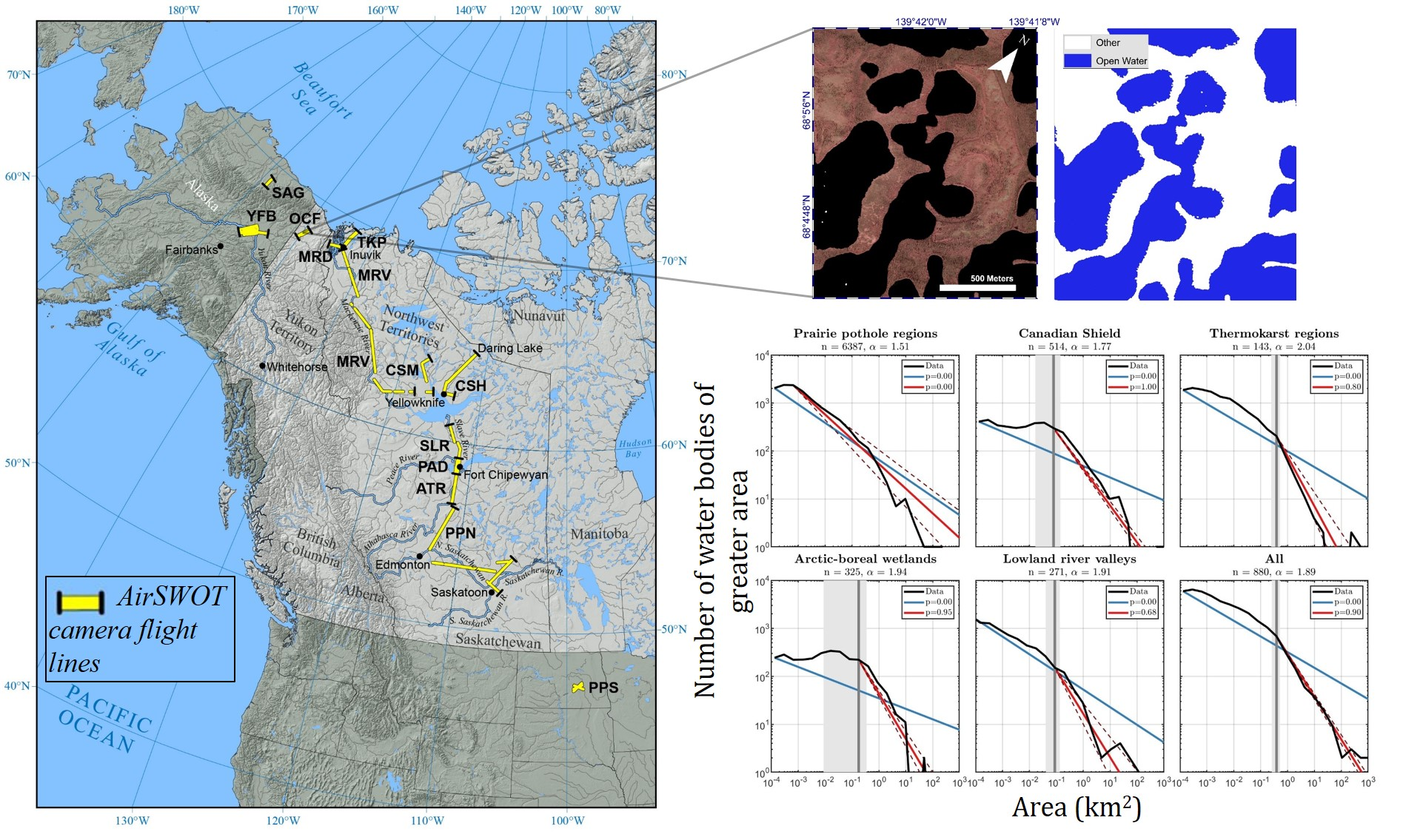
2.1. 2017 ABoVE AirSWOT Study Areas and Flight Lines

ABoVE AirSWOT deployments occurred in two legs, with northbound sorties from North Dakota to Alaska conducted between July 9–21, 2017 and southbound sorties over the same flight lines from August 6–17, 2017 (Figure 1). Overlapping flight lines were designed to cover key field sites and to provide repeat-pass data to support model-, field-, and satellite-based studies [33]. The areas imaged by AirSWOT include the Yukon Flats Basin (YFB), a floodplain wetland environment along the Yukon River, near Ft. Yukon, Alaska, the Mackenzie River Delta (MRD), Northwest Territories (NWT), Canada, Precambrian Canadian Shield lakes (CSH) near Yellowknife, NWT, the Peace-Athabasca Delta (PAD), Alberta, the largest inland delta in North America, and prairie pothole lakes in Saskatchewan and North Dakota (

Table 1. Study regions, acquisition dates, and coverage areas of 2017 ABoVE AirSWOT color-infrared camera image acquisitions. The designation “river valley” refers to sorties roughly following a lowland river or river valley. The designation “wetland” refers to Arctic-Boreal wetlands (including river deltas), and “pothole” refers to glacially formed, prairie pothole lakes.

Region	Site Code	Category	Area (km2)	Northbound Flight(s)	Southbound Flight(s)
Sagavanirktok River	SAG	Lowland river valley	309	July 19	-
Yukon Flats Basin	YFB	Wetland	4601	July 17, 20, 21	August 6, 7
Old Crow Flats	OCF	Thermokarst	653	-	August 7
Mackenzie River Delta	MRD	Wetland	409	July 16	August 7
Tuktoyaktuk Peninsula	TKP	Thermokarst	1095	July 16	August 9
Mackenzie River Valley	MRV	Lowland river valley	3748	-	August 9
Canadian Shield Margin	CSM	Wetland	814	-	August 9, 12
Canadian Shield	CSH	Shield	2183	July 15	August 12, 15
Slave River	SLR	Lowland river valley	878	-	August 13
Peace-Athabasca Delta	PAD	Wetland	1509	-	August 13
Athabasca River	ATR	Lowland river valley	1011	July 9	August 13
Prairie Potholes North	PPN	Pothole, Lowland river valley 1	5289	July 9	August 16,17
Prairie Potholes South	PPS	Pothole	880	-	August 17
All regions	-	-	23,380	-	-

¹ This region transitions from a sparsely-populated, forested region in the north to agricultural prairie pothole lakes in the south.

). Mean precipitation (1979–2010) for these areas ranges from 155–471 mm and mean annual air temperatures range from −13.6 to 4.4 °C [34]. Summer 2017 mean precipitation less evaporation (P-E) along the AirSWOT flight lines is generally negative, averaging −1.2 mm in July and −0.2 mm in August [34], with corresponding lake area decreases between the two acquisition dates.

2.2. CIR Camera Image Acquisition and Processing

2.2.1. Image Acquisition

The 16-megapixel (MP) CIR camera was mounted in a NASA B200 King Air and enclosed in a box fitted with a 16-inch diameter glass window. Mapping flights occurred at roughly 8–11 km altitude with a target along-track overlap of 60% and variable across-track overlap. For flights prior to 29 July 2017, data were collected with a fixed-length, 60 mm lens with a 34° field-of-view. Individual raw image dimensions were 4072 × 4072 pixels before mosaicking. For flights after 29 July 2017, data were collected with a fixed-length 80 mm lens with a 25° field-of-view. The auxiliary shutter on these cameras sometimes malfunctioned, resulting in only partial shutter opening, which increased vignetting at the top and bottom of raw images. To minimize vignetting effects for orthomosaic generation, raw images were clipped, resulting in final dimensions of 4072 (width) × 3472 (along-track) prior to image-stitching and orthorectification. Raw images having less than 50% cloud cover were digitally stitched and orthorectified in Agisoft PhotoScan 1.3.4. Out of 22,631 raw images acquired, 7086 were used to create 38 orthomosaics, each pertaining to a specific ground area flown on a single day. On average, each ground pixel in an orthomosaic was imaged 5.7 times from different angles. The orthomosaics were resampled to 1 m pixels from a native resolution ranging from 0.92 to 1.32 m.

2.2.2. Image Quality

Atmospheric conditions and mechanical failures caused challenges during the 2017 AirSWOT ABoVE sorties. Approximately one-third of the final images contain some clouds or cloud shadows. There are missing data values due to insufficient photogrammetric pixel correlations between raw image overlaps, typically over clouds, uniform lakes, and moving water. Most missions were flown during morning hours, where shifting solar conditions resulted in illumination inconsistencies between paths during individual missions, as well as fog. No atmospheric or illumination correction was applied, leading to subtle striping effects, with each stripe occurring along the track of a flight path. Per standard practice, the camera was integrated with the aircraft without consideration for circulation of warm air across the camera window, which resulted in ice and condensation on the lens during operation. These effects resulted in small, dark spots over some areas (appearing as roughly 10 m² patches on the ground). Despite these limitations and lack of radiometric calibration, the imagery is suitable for mapping fine-scale water bodies and other features on the land surface.

2.2.3. Geolocation Correction

The CIR orthomosaics were initially georeferenced using aircraft positional data (IMU and GPS). Initial orthomosaics had geolocation offsets ranging from 0–120 m between identical ground points imaged on different days. These offsets were resolved by manually georeferencing 29 orthomosaics using 303 user-selected ground control points (GCPs). The remaining nine orthomosaics had negligible registration errors, so no correction was needed. GCPs were manually digitized from the Digital Globe EV-WHS image service, which provides orthorectified imagery with spatial resolutions of ≤1 m [35]. The four operational Digital Globe satellites [36] used as input to the service have a 90th percentile geolocation error ranging from 3.0 m (GeoEye-1 satellite) to 6.5 m (Worldview-1 satellite) [36]. GCPs were chosen as persistent landscape features identifiable in both the orthomosaics and the Digital Globe image service, including road intersections, tree stand boundaries, and shorelines from water bodies having stable sizes and shapes. Images were warped using a 1st-order polynomial (affine) transformation in ArcMap 10.6, and the average and root-mean-squared average distances between the source and map GCPs were computed. If they differed by more than 20%, the image was split into two or more parts and the warp re-applied using the corresponding subsets of GCPs. These operations were performed on the original orthomosaics using the same geographic coordinate system as the DigitalGlobe service (WGS-84).

After georeferencing, 90% of GCPs deviated from DigitalGlobe by ≤13.3 m (13.3 pixels) (Figure 2). Including the accuracy of DigitalGlobe, the horizontal accuracy of the CIR imagery and masks is 19.8 m or better for 90% of the images. The 38 orthomosaics were then projected to Canada Equal Albers Conic and split to the ABoVE grid C [30], yielding 330 orthomosaic images in geotiff (.tif) format. Individual image accuracies are included in the data sets [37].

2.3. Open Water Classification

We designed a semi-automated image classifier to identify open water unobscured by aquatic or riparian vegetation, algae, and built objects (hereafter referred to as open water). This conservative classification yields a water body product uncontaminated by vegetation or other material that could bias the water surface elevation retrievals obtained from coincident AirSWOT Ka-band interferometric radar images. This conservatism, along with synchronous acquisition with Ka-band radar imagery, makes the CIR dataset presented here optimal for AirSWOT studies of surface water extent and elevation.

In some cases, the restrictive classification causes patches of open water within a vegetated lake to appear as individual water bodies. To mitigate these effects, polygon aggregation was used to ensure each mapped open water body had a one-to-one relationship with the lake, pond, or wetland feature it represented (Section 2.5). Other effects such as clouds, shadows, and lack of atmospheric correction that complicated the optical classification are noted (along with quality metrics) for each classified image. To assess the effects of this area-measurement method on open water area, the high-resolution CIR mask was compared to typical lake area measurement from the global lake database HydroLAKES [38]. Open water areas were correlated (r² = 0.62), as determined by comparing 729 lakes greater than 0.1 km² with their full extents imaged by the CIR camera. In general, although the two water body definitions differ, these results still provide insight into the distribution of lake areas.

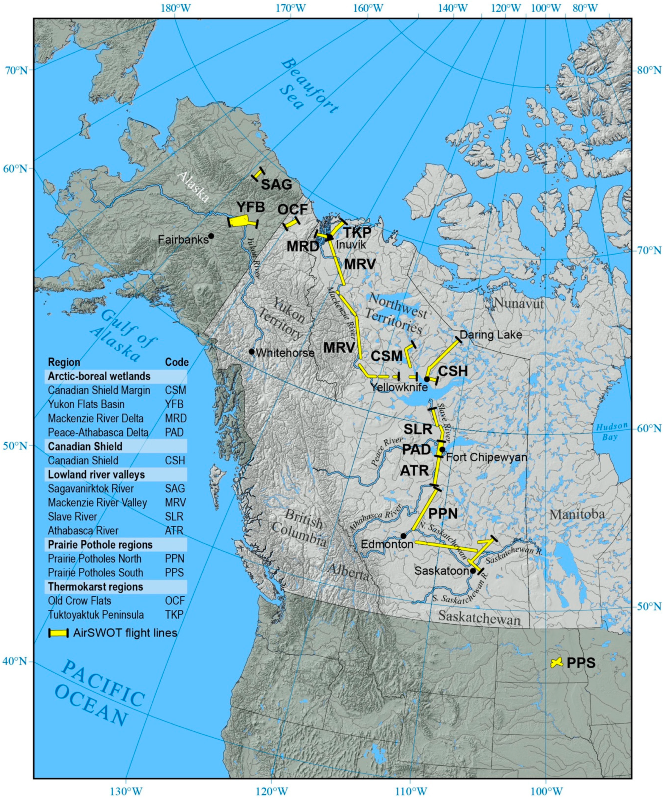
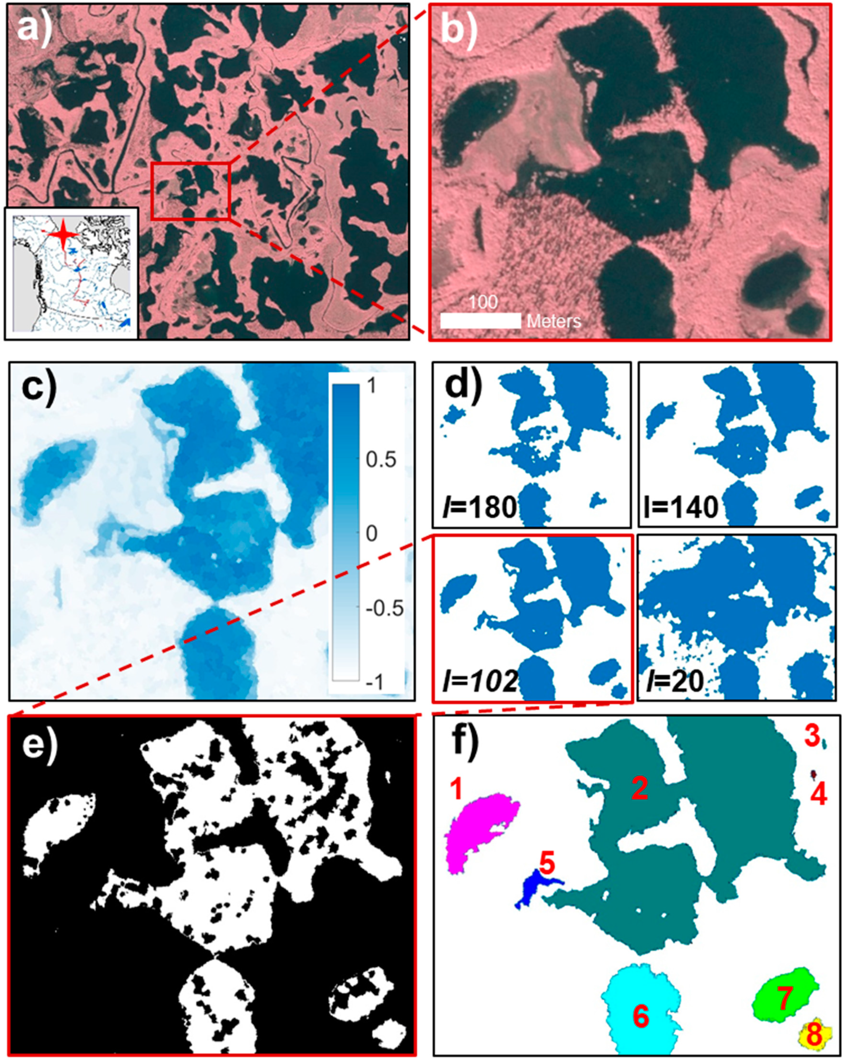
2.3.1. Automated Classification Steps

The open water classifier (Figure 3) is based on the Normalized Difference Water Index (NDWI) [39], a normalized ratio of the near-infrared and green bands. In some cases, classification was improved by using only the near-infrared (NIR) band instead of the NDWI. Prior to classification, each orthomosaic image was split into processing tiles of ~ 40 km² to conserve memory and over-segmented into pixel-cluster objects, also called superpixels. Known as object-based image classification (OBIA), this procedure is a common technique in image [40,41,42] and water [43,44] classification. For the segmentation, the simple linear iterative clustering with zero parameters (SLIC0) algorithm was used [45], implemented in Matlab 9.4, with a scale (controlling the average size of a cluster) of 100 pixels (100 m²). The resulting clusters ranged in size from 20 (small, uniform regions, such as ponds) to 500 pixels (no-data boundaries, featureless water patches or fields) and served as the basis for the classification. Our choice of algorithm and parameters was informed by a previous study [46] and prevents clusters from being larger than the smallest observable water bodies.

Next, each processing tile was assigned an optimal global NDWI or NIR threshold as per the connectivity-preserving algorithm of O’Gorman [47]. This step maximized the number of connected regions without inducing noise by selecting too many total regions. To account for images with varying backgrounds, the original algorithm outputs several intensities that can be used to binarize the tile. Here, we modified it to produce only one output level (representing the optimal cutoff between open water and land), given an a priori range of user-selected plausible thresholds. This algorithm has previously been implemented for remote sensing of landslides [48], ocean vessels [49], and sea ice [50]. Here, we present its first application to remote sensing of inland surface waters.

A local water index threshold was computed for each potential water body in the resulting binary image [51,52,53]. First, clusters with rough textures were removed, as indicated by their entropy value [54], a statistical measure of randomness. High-entropy regions generally occur along shorelines and are analogous to mixed-pixels, so this operation morphologically erodes the edges of water bodies. Next, region-growing, based on the mean and standard deviation of the local water index, was applied to each eroded region. Adjacent pixel clusters were included if their mean value fell within two standard deviations of the mean value of the region. To produce the final open water mask, data gaps surrounded by water were reclassified as water, and small regions (<40 pixels) were removed to reduce commission errors caused by tree and terrain shadows.

2.3.2. Manual Classification Steps and Quality Assessment

After running the open water classifier, each classified image was visually inspected for clouds, haze, or other image quality concerns that prevented accurate image classification. Two post-classification adjustments were made to address image quality. First, the processing tile aspect ratio was adjusted to values between 1:1 and 1:2 for tiles with narrow data coverage due to linear flight lines. This approach was most effective on tiles covering ~5 km² or less lacking representative samples of both land and water classes. Second, the a priori upper and lower NDWI bounds used for the connectivity-preserving binarization were varied between −0.72 to −0.39 (lower) and 0.48 to 0.78 (upper). This change was necessary for images containing roads and buildings, whose superpixels were morphologically connected and were, thus, preferentially selected in the connectivity-preserving binarization. These procedures were then repeated until satisfactory results were obtained. For 30 of the images, the NIR band was used for the classification instead of the NDWI in order to avoid false positives. In total, approximately half of the 330 CIR images required re-processing.

2.4. Validation of Open Water Classification

Classification error was quantified by manually digitizing water bodies and computing a confusion matrix [55]. Since the imagery contained mostly land, a random pixel-based validation scheme would not have included enough water pixels. Instead, 197 open water bodies were selected from six validation areas across the study area, including one of the areas visited in-situ. Boundaries were digitized solely around open water to avoid mixed pixels, using a consistent image stretch between regions. These digitized polygons were then rasterized and confusion matrix statistics calculated on a per-pixel and per-water-body basis between the manual and classified water bodies.

The CIR open water classification was further validated against in situ shoreline surveys of 26 lakes and rivers islands. These shorelines were surveyed using a handheld Garmin eTrex GPS with horizontal accuracy ~3 m. Surveys were conducted in YFB, CSH, and PPN within 30 h of CIR image acquisition (with the exception of YFB, which was collected 73 h after the flight). In areas of emergent aquatic vegetation, the outermost wet shoreline was mapped. Although this technique did not necessarily capture open water boundaries, it provided an independent verification of the maximum shoreline extent.

2.5. Water Body Morphometric Analysis

From the classified images, open water area for each cloud-free water body was computed and stored as a shapefile (.shp) attribute. Water masks from these image files were converted to polygons with adjacent boundaries dissolved to account for water bodies split between different files. Rivers and incomplete lakes were removed by deleting polygons that intersected the study region boundaries, with the rest removed based on visual inspection. Finally, water bodies within 20 m of each other were aggregated so that those erroneously appearing discontinuous due to vegetation were counted as one, and the final polygons were stored as a single shapefile (Figure 4). The conservative 20 m distance was chosen to avoid aggregating neighboring ponds when they should be treated separately. The resulting shapefile used for analysis covers 21,644 km² (37.7%) of the ABoVE foundational flight areas and contains only open water bodies not connected to river networks.

Since some imaged lakes were too wide to be fully observed in an AirSWOT flight line, lake polygons falling across image boundaries were fused with the HydroLAKES database [6] before analysis. This approach increased the range of documented lake sizes by an order of magnitude and removed a sample bias towards small water bodies. As the study area includes lakes as large as Point Lake and Eskimo Southern Lake on the Canadian Shield (977 and 843 km²), this fused dataset includes lakes from all size classes intersected by 2017 AirSWOT flight lines across Arctic-Boreal Alaska and Canada.

2.6. Power-Law Scaling of Water Body Area Distributions within Physiographic Subregions

We categorized the study area into five dominant, physiographic classes (Arctic-Boreal wetlands, Canadian shield, lowland river valleys, prairie pothole lakes, and thermokarst) and 13 smaller sub-regions (SAG, YFB, OCF, MRD, TKP, MRV, CSM, CSH, SLR, PAD, ATR, PPN, PPS, Figure 1 and Table 1). This categorization enables statistical comparisons of water body morphology and area distribution across a variety of typical Arctic-Boreal landscapes and spatial scales. A summary of the acquisition dates, physiographic categorization, and flight line areas is presented in Table 1.

To analyze the scaling behavior of mapped water bodies within these various sub-regions, we tested the hypothesis that surface water body area distributions follow a power-law [23]. Maximum-likelihood estimation (MLE) was used to estimate the most probable value of α and the most probable onset (if any), A₀, of power-law behavior in the area distribution. The MLE estimation was performed for each sub-region (n = 13), physiographic terrain class (n = 5), and over the entire dataset [56,57,58]. To understand how the choice of sub-region boundary might have influenced sampling, a bootstrap method [59] was used to estimate p-values and one-standard-deviation confidence intervals for α and A₀ as follows: 1000 subsets for A > A₀ were generated using the MLE estimates of α.

Finally, p-values for α were estimated using the Kolmogorov-Smirnov (KS) statistic [56]. Each MLE estimate of α was used to construct 1000 random distributions of P(A) for A > A₀, and p-values were estimated as the fraction of those distributions with KS statistics that were further away from the true power-law distribution. We defined statistical significance as p < 0.1, meaning mapped water body size-distributions were further from a true power-law than 10% of the synthetic datasets and the non-power-law null hypothesis was supported. This procedure was repeated with A₀ set to the minimum water body area to test for power-law behavior across the full range of A.

3. Results

3.1. Validation of the Open Water Classification

As expected, the open water classifier performed best on CIR images free from clouds, haze, shadows, and mosaicking artifacts. From manual inspection (Section 2.3.1), features including roads, buildings, shadows, and agricultural fields were sometimes incorrectly classified as water. PPN and PPS had the highest commission error due to human-made features, whereas CSH and CSM had the highest commission error due to tree-shadowing. Omission error can most often be attributed to the spectral properties of turbid water (e.g., sediment-rich rivers resembling the spectrum of concrete), especially if found within the same scene as clear water. The classification performed poorly over industrial ponds in the oil sand extraction regions of northern Alberta due to their extremely high turbidity. Misclassification of gravel bars was mitigated through the use of O’Gorman’s connectivity- preserving algorithm [47], which performed better in an object-based framework than the popular Otsu method of maximizing between-class variance [60] (Figure 5). The classifier also did not perform well on narrow streams (<15 m wide), likely due to overhanging riparian vegetation and a high percentage of mixed pixels. However, remaining streams were manually removed and not used for the area scaling analysis (Section 2.4).

The 197 open water bodies used for manual digitization have a total area of 3.09 km²_. The equivalent areas in the classified product contain 200 water bodies, with a total area of 3.34 km². Thus, the classifier demarcated more water body area (7.7% difference), and slightly more water bodies overall (1.5% difference). The overall accuracy is 98.0%, with user’s and producer’s accuracies of 87.1% and 94.0%, respectively, and a kappa coefficient of 89.3% (

Table 2. Confusion matrix between 197 manually digitized water bodies and the automated open water classification (units in m², and percentage of pixels). Evaluation areas came from six geographically distributed regions (YFB, OCF, MRD, CSH, PAD, PPN).

		Reference
		Other	Open Water	Row Total	User’s Accuracy
Map	Other	27,245,985	184,418	27,430,403	99.3%
	Open Water	431,610	2,904,932	3,336,542	87.1%
	Column Total	27,677,595	3,089,350	30,766,945
Producer’s Accuracy		98.4%	94.0%		98.0%

and

Table 3. Summary accuracy metrics for open water detection. Negative percent differences imply larger values for the classified water (map) than the digitized water (reference).

Error Metric.	Percentage
User’s Accuracy	87.1
Producer’s Accuracy	94.0
Overall Accuracy	98.0
Kappa Coefficient	89.3
Area percent difference	−7.7%

). As noted in Section 2.4, validation regions were digitized extremely conservatively, so the 7.7% extra classified areas represent an upper bound.

Walked shorelines are inland of or equal to the classified shorelines for vegetated lakes, implying that the classifier conservatively mapped open water (Figure 6a,b). The classified shorelines of non-vegetated sandbars (Figure 6c–f) are also generally inland of walked shorelines, implying omission errors from water resembling wet sediment or changing water levels (the Yukon River surveys were conducted days after the flight). The maximum Euclidean distance between classified and walked shorelines is 45 m in the Yukon River sandbars, 16 m in the North Saskatchewan River, and 15 m for the ponds in PPN. Thus, the in-situ surveys provide a ground-verified reference to assess uncertainty in shoreline locations.

3.2. CIR Camera Water Body Classification Summary Statistics

The CIR open water classification identified 43,562 water bodies with areas ranging from 40 m² to 15 km². The total open water extent mapped (F_water) is 2885 km², or 12.34% of the 23,380 km² study area, varying from 2.57% in SAG to 37.60% in MRD. The portion of the landscape occupied by lakes and wetlands (i.e., with rivers removed, F_lakes) is 7.71%, varying from 0.36% in SLR to 23.3% in CSH. The median water body area (A_med) is 0.0007 km² (700 m²), varying from 0.0003 km² (300 m²) in SAG to 0.008 km² (8000 m²) in TKP. These results show considerable variation in morphometry between sub-regions, largely driven by physiographic setting.

These data are presented as 330 raster files, 236 of which are free from significant classification errors due to clouds or haze. Also included in the dataset are: (1) a shapefile with attributes denoting geolocation accuracy, classification quality and the presence of clouds or haze; and (2) a shapefile containing classified water bodies, with areas given as an attribute. Data are freely available for download via the Oak Ridge National Laboratory (ORNL) Distributed Active Archive Center (DAAC) for Biogeochemical Dynamics at https://doi.org/10.3334/ORNLDAAC/1707.

3.3. Area Distributions of Mapped Water Bodies

Water body area distributions confirm the abundance of small water bodies (Figure 7), particularly those with areas <0.001 km², which is the lower limit of current global studies [8,15,26]. Of the 43,562 classified water bodies, 56.2% are <0.001 km², comprising 3.46 km² or 0.12% of total open water area (

Table 4. Regional distribution statistics for 43,562 mapped water bodies. N is the number of water bodies in the region, A_med is the median area, F_water and F_lakes are the fractions of area covered by open water and lakes/ponds, F_0.001 is the fraction of water bodies of areas <0.001 km² in area, A_0.001 is the fractional contribution to total area from water bodies <0.001 km², A₀ is the water body area that produces the best goodness-of-fit for a power-law distribution based on water bodies of greater or equal-area (standard deviation σ_A0), α is the power-law exponent taken for areas A₀ and greater (standard deviation σ_α), and p is the p-value from the power-law fitting test, considered for water bodies larger than A₀. Regions having p values less than 0.1 (in bold) are rejected as power-law distributions.

Region	Area (km2)	N	Amed (m2)	Fwater (%)	Flakes (%)	F0.001 (%)	A0.001 (%)	A0 (m2)	σA0 (m2)	α	σα	p
SAG	309	532	300	2.57	0.68	74.62	3.03	502	193	1.61	0.05	0.72
YFB	4601	8508	892	7.13	3.45	51.97	0.77	273,396	96,159	2.51	0.28	0.88
OCF	653	1208	4522	20.94	18.41	36.01	0.07	216,520	102,553	1.94	0.12	0.85
MRD	409	2305	1746	37.60	22.47	43.47	0.21	250,581	145,859	2.18	0.32	0.69
MRV	3748	4670	615	17.34	4.06	56.27	0.16	83,734	68,758	1.89	0.15	0.23
CSM	814	1271	644	11.81	10.87	57.28	0.03	6502	6093	1.59	0.07	0.99
CSH	2183	4136	3012	23.95	23.30	39.58	0.02	117,629	62,699	1.77	0.04	1.00
SLR	878	720	374	12.74	0.36	68.47	3.08	1942	1456	1.83	0.12	0.86
PAD	1509	2293	284	10.93	6.77	71.52	0.22	1115	1582	1.62	0.05	0.42
ATR	1011	1193	226	5.30	1.80	77.20	0.61	351	1214	1.60	0.08	0.14
PPN	5289	13,013	415	5.21	4.33	67.69	0.35	-	-	-	-	0.00
PPS	880	1770	1427	10.29	8.99	45.03	0.33	544,824	78,690	2.41	0.18	0.97
TKP	1095	1943	7976	26.79	22.78	29.28	0.01	254,009	181,073	1.95	0.14	0.93
Pothole	5822	13,758	520	6.09	5.26	63.00	0.33	-	-	-	-	0.00
Shield	2183	4136	3012	23.95	23.30	39.58	0.02	117,629	61,817	1.77	0.04	1.00
Wetland	7333	14,377	770	10.13	6.01	54.20	0.19	458,480	141,329	2.04	0.20	0.80
Thermokarst	1748	3151	6820	24.61	21.15	31.86	0.02	235,093	167,851	1.94	0.09	0.95
River valley	6293	8140	356	13.27	2.82	66.06	0.28	94,158	47,170	1.91	0.20	0.68
All	23,380	43,562	665	12.34	7.71	56.19	0.12	343,074	130,800	1.89	0.04	0.90

). The fraction of water bodies under this threshold (F_0.001) is 56% and ranges from 29% in TKP to 77% in ATR.

Most sub-regions have scale-invariant tails to their area distributions (Table 4), as shown by the linear portions of their cumulative distribution functions (CDFs, Figure 8 and Figure 9). A power-law distribution is plausible for water bodies >0.34 ± 0.13 km² across the entire study region, representing 1.5% to 3.2% of water bodies by count and 89.6% to 93.4% by area. Scaling estimates pertaining to the remaining water bodies would thus, remain highly uncertain. Regionally, all categories except for the prairie pothole region PPN (p = 0.00) could fit a power-law for A₀ ranging from 0.00050 (SAG) to 0.54 km² (PPS). Although PPN appears linear on a log-log plot, its much larger sample size (1–2 orders of magnitude larger than the other sites) provides more data points for the maximum-likelihood estimation (MLE) to rule out the power-law hypothesis, so this finding should be interpreted with caution. The hypothesis is plausible for other sub-regions, with the onset of power-law scaling A₀ ranging from 350.5 m² (ATR, 99.18 to 100.00% of water bodies) to 0.54 km² (PPS, 59.16 to 64.5%). Finally, CSH is indistinguishable from a power-law in the tail end of the distribution (p = 1.00). The power-law scaling exponent α varies from 1.59 (CSM) to 2.51 (YFB), with a value of 1.89 for the entire study area. The variability in A₀, α, and p suggest that a single power-law distribution does not apply to the areas classified here, as supported by the non-linear curves in Figure 8.

Based on the power-law exponent α, the regions analyzed generally fall into two end-members, with wetlands and thermokarst having the greatest α values (1.94 to 2.04) and pothole lakes having lower α values (1.51) and thus a flatter distribution. However, values between sub-regions PPN and PPS differed by 43%, implying contamination from other types of driving physiographic factors. This contamination was most prevalent in the larger and more heterogeneous PPN region, which transitions from sparsely populated boreal forest in the north to agricultural regions with constructed lakes in the south. The high-α end members make sense since the two thermokarst regions, TKP and OCF, contain seasonal tundra wetlands. The remaining regions, Canadian Shield and lowland river valleys, had intermediate α values (1.77 to 1.91). Coarse-scale water body maps in regions with large α values would be most affected, as they have a greater proportion of small water bodies, and, indeed, wetland regions have both high α values and a high A₀. The two prairie pothole sub-regions in aggregate (PPN and PPS, Figure 9) and PPN individually did not fit a power-law distribution (p = 0.00), and they had among the highest percentage of small water bodies, making their abundance difficult to estimate from coarse-scale maps. In contrast, shield lakes very likely fit a power-law distribution (p = 1.00) and had low A₀ values, implying that coarse-scale information in these regions could be sufficient to estimate water body abundance.

This analysis has a strong dependence on how sub-regions are constructed; thus, distributions at three spatial scales were analyzed (Section 2.5). In general, as the number of water bodies grows, p decreases, although sample size only explains a small percentage of the variation (r² = 0.11, Figure A2). This effect results from smaller regions being more likely to have an unvarying distribution across their spatial domain. Spatial variability within regions could cause the slope breaks seen in the category-scale plots (Figure 8) and might also explain why the power-law hypothesis was rejected for PPN. This sub-region is 1–2 orders of magnitude larger than the others and includes numerous agricultural ponds and impoundments, as well as glacially-formed prairie pothole lakes. The variance among the fitted α and A₀ parameters indicates that sub-region divisions captured boundaries between hydrologic landscapes. Thus, there is a preferential scale for power-law fitting analyses, determined by landscape physiography, and biases can be reduced by analyzing multiple scales to prevent arbitrary sub-region divisions from impacting results.

4. Discussion

This study builds on prior studies of open water classification [11,61,62] and area distribution scaling [6,23,63] using spaceborne and airborne color-infrared digital imagery by: (1) advancing a new, high-resolution AirSWOT color-infrared (CIR) camera dataset and open water classification for the NASA Arctic-Boreal Vulnerability Experiment (ABoVE); (2) applying the connectivity-preserving binarization technique [47] and an object-based framework to classify open water in the CIR dataset; (3) using the classification to map small (<0.001 km²) water bodies over physiographic gradients; and (4) testing whether the mapped water body area distributions display scale-invariant power-law behavior, with a focus on selecting the appropriate area domain. Each of these four contributions is discussed next.

4.1. Utility of CIR Open Water Classifications for the SWOT Satellite Mission

AirSWOT was developed as a calibration-validation platform for the forthcoming NASA Surface Water and Ocean Topography (SWOT) satellite mission (https://swot.jpl.nasa.gov/), anticipated to launch in 2021 [64,65]. A key SWOT mission objective is to obtain water surface elevation (WSE) to ±10 cm vertical accuracy for 1 km² open water regions [66]. Previous work used CIR-derived water masks and spatially-averaged AirSWOT Ka-band interferometric radar data to estimate AirSWOT WSE accuracies of ~9–10 cm in rivers and ~21 cm in lakes [53,67,68,69]. The conservative AirSWOT color-infrared (CIR) water mask provided here should enable unambiguous extraction of open water pixels used for spatial averaging of AirSWOT interferometric radar data, and, therefore, improve estimates of WSE accuracy (Figure 10). CIR imagery would also help identify phenomenology issues that should be excluded from spatial averaging of AirSWOT radar data, for example, exclusion of wet sediment bars as noted in Section 3.1, which could introduce height errors if erroneously classified as open water. Similarly, the presence of emergent aquatic vegetation may be identified by overlaying AirSWOT backscatter on CIR imagery. In general, the synchronicity and co-registration between the AirSWOT CIR camera and Ka-band interferometric radar is a powerful combination for accurate mapping of surface water extent and WSE. Paired AirSWOT CIR and InSAR imagery thus provide an effective way to validate both surface water extent and WSE during the forthcoming SWOT mission.

Several improvements to the AirSWOT camera system are recommended to further improve the value provided by this system. The CIR camera image registration could be improved by upgrading the positional and image timestamping systems, increasing the overlap between flight paths (to assist photogrammetric correlation), or both. Adding an additional spectral band in the mid-range infrared (1500–2000) nm would improve identification of water, which cannot be detected by the current 760–900 nm sensitivity. Including these wavelengths would permit the use of spectral indices such as the Automated Water Extraction Index (AWEI) [70] and Modified Normalized Difference Water Index (MNDWI) [71] which provide better contrast between land and water pixels, especially over human-influenced landscapes. Absolute radiometric calibration and solar illumination correction would also improve automated open water classification by enhancing consistency between images. Finally, the classifier presented here should be modified to improve automation and deliver a quicker product. These modifications would permit timely validation of SWOT-observed water extent over large areas where AirSWOT is flown during the proposed satellite mission.

4.2. Utility of CIR Imagery and Open Water Classifications for the NASA Arctic-Boreal Vulnerability Experiment (ABoVE)

AirSWOT CIR imagery and open water classifications also hold value for other flight campaigns conducted for the NASA Arctic-Boreal Vulnerability Experiment (ABoVE). The 2017 AirSWOT flight lines described here were designed to maximize overlap with other ABoVE airborne campaigns, including LVIS, UAVSAR, AIRMOSS, AVIRIS-NG, and CFIS. The user-friendly CIR image catalog and manually derived cloud flags enable end-users to locate high quality, high-resolution images over areas targeted by other field and remote sensing investigations [37]. The high-resolution open water classification presented here [73] may provide a useful dataset for studies exploring links between surface hydrology and permafrost [53,74], ecosystem services [75], and carbon cycles [18,76] that currently rely on satellite products, lake censuses, or other coarse-resolution open water maps.

To illustrate this cross-discipline utility, we overlay the CIR open water mask with UAVSAR polarimetric L-band SAR data (Figure 11). Given its relatively long wavelength of 23.8 cm, L-band radiation can penetrate moderately dense vegetation and give strong double-bounce returns off vertical wetland vegetation emerging from the water surface. The CIR imagery helps identify this vegetation, and the open water mask can be used to identify the extent of emergent vegetation where double-bounce returns begin. This dual-sensor information can be used to map the entire surface area of lakes with higher confidence than either sensor alone. Although not available at this time, a combined product would minimize counting errors associated with disconnected open water patches and allow water to be partitioned between open and vegetated regions.

The CIR imagery may also add value to studies using the hyper-spectral sensor AVIRIS-NG and the waveform LiDAR sensor LVIS. For example, patterned ground features such as fine-scale polygonal networks and ponds caused by permafrost thaw are barely detectable in 5 m-resolution AVIRIS-NG imagery and are easier to resolve in the high-resolution CIR imagery (Figure 12). Although too small to be detected by the classifier, the raw CIR imagery resolves small ephemeral ponds formed above thawing permafrost that are important to the permafrost-carbon feedback [77]. The hyperspectral capabilities of AVIRIS-NG offer the potential to study vegetation, water quality, trace gases, snow, soil, and other systems [33]. The CIR open-water mask could also aid interpretation of 1064 nm laser backscatter from open water as from LVIS and together could offer an independent method for partitioning open and vegetated water surfaces. High-resolution digital elevation models (DEMs) provided by this sensor can enhance fine-scale runoff modeling and studies involving ephemeral water bodies. These synergies present opportunities for more precise water and vegetation mapping using concurrent ABoVE datasets.

4.3. Validated Open Water Classification Performance

The accurate water classifications obtained here suggest the object-based, connectivity-preserving classifier is well-suited for open water mapping. As noted by O’Gorman [47], pixel connectivity is a local measurement used for a global threshold, with the advantage that all regions of the image are used when choosing a threshold. Although this technique was originally developed for document image scanning, it works well for mapping open water bodies, which exhibit pixel connectivity just like letters in text. Moreover, we applied this technique to an object-based framework and demonstrated that small shadows and speckle noise in the uncalibrated imagery are evened-out. Working with pixel regions rather than pixels reduced the size of the data set, which saved memory and resulted in a reasonably fast processing time of about four minutes for a 50-million-pixel processing tile (using a 3.7 GHz Intel Xeon processor with 16 GB of RAM). As in other high-resolution studies [32,51], classifications were manually edited to remove false-positives caused by shadows and other factors.

We took a conservative approach to validation, using manually-delineated water body shorelines and in-situ mapping. Consequently, the classifier is more likely to miss than falsely identify water. This is supported by most classified open water boundaries falling inside walked shorelines (Figure 6) in areas with littoral zone vegetation. The lower user’s accuracy (87.1%) than producer’s accuracy (94.0%, Table 2) is indicative of the conservative boundaries used for digitization. In addition, the 40 m² size limit and the spectral limitations of the camera exclude narrow streams. Optical classification of the stream and river channels is difficult due to the necessity of producing continuous networks from narrow regions [81]. In addition, the process of creating a binary water mask is subjective. Even ground-based shoreline surveys may incorrectly identify shorelines obscured by vegetation or saturated sediments. In general, we found that small water bodies (<0.001 km²) are particularly challenging for high-resolution water classification, as vegetation often obscures shorelines, making individual water bodies hard to count. Furthermore, these small water bodies are the most ephemeral. More work is needed to create multi-temporal products and understand seasonal variation.

4.4. Improving Mapping of Very Small Water Bodies

Small water bodies are important for methane release [82,83], biodiversity [22], and organic matter burial [22], but are under-represented in studies limited by the spatial resolution of Landsat or coarser sensors [8,21,22]. One approach to solving this problem is the use of scale-based estimates, but such estimates may not apply at small scales [24]. Remote sensing offers the only consistent method to identify these water bodies globally, but most space-borne sensors lack sufficient spatial resolution to test for scale-invariant behavior over all size scales. This dataset provides much-needed information on the distribution of these small water bodies in Arctic-Boreal North America.

Waterbody size metrics, such as area and shoreline length, could be valuable for earth system models that use coarse water cover fraction as an input. Inaccuracies in wetland maps used for methane models have been attributed to both undercounting [84] and double-counting by inclusion with lake classes [85]. For models too coarse to resolve small water bodies, the fractions A_0.001 or similar perimeter metrics could be used to upscale the processes that occur in small ponds or wetlands. Accurate water body maps are crucial to improving methane emission estimates from models, so upscaling approaches may represent one way to transfer fine-scale information to coarse-scale maps used for models [8,38,82]. In Alaska, high-resolution imagery has been used to upscale methane fluxes based on vegetation mapping [86], and these techniques can also be applied to water and wetland maps. The CIR imagery and open water masks cover large areas at high resolution and offer a valuable airborne-scale census of surface water over a variety of landscapes.

Boundaries used to define representative areas can influence conclusions drawn about enclosed small water bodies. Regionally, the Canadian Shield and thermokarst landscapes had the highest overall water fraction (14.4%), which is consistent with other work [6,23,38]. For the YFB, we find F_0.001 is 52%, whereas McDonald et al. [15] found 28%, using a region five times smaller and different procedures for defining small water bodies. This discrepancy highlights the sensitivity of morphometric analyses to study area boundaries.

The contribution of small water bodies <0.001 km² to total water area has been considered negligible [82], on the order of fractions of a percent, and our findings of 0.12% for the entire study domain support this conclusion. However, river valley sub-regions such as SAG and SLR have A_0.001 > 3%. Ponds below 0.001 km² are estimated to make up 6–11% of the global surface area of lakes and ponds, yet comprise up to 23% of CO₂ emissions and 70% of diffusive CH₄ emissions from lentic freshwaters [83]. They tend to have higher rates of carbon burial, fish productivity, and waterfowl, amphibian, plant and fish species richness than larger lakes [22]. They can also provide ecosystem services such as small-scale water supply and nutrient processing [21]. Thus, the fraction of small water bodies observed is not negligible for a variety of carbon cycle and ecosystem processes.

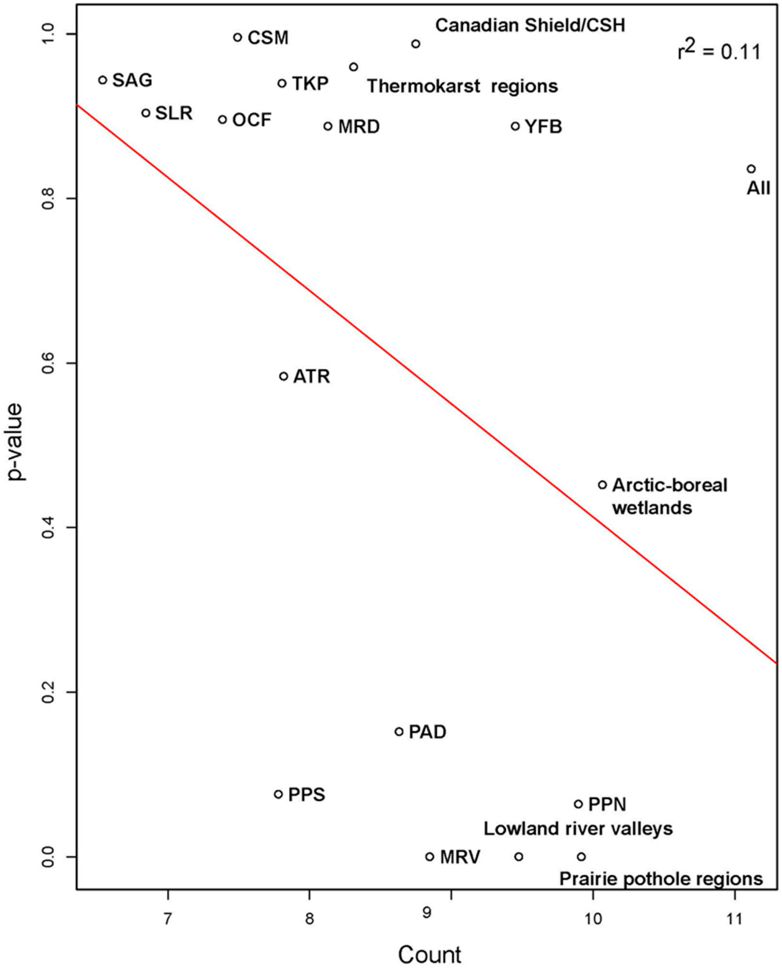
4.5. Testing Power-Law Regimes

The power-law hypothesis for lake size distribution is often invoked [7,16,20,23,25,26] but lacks rigorous tests on its adequacy for modeling small lakes. Log-log slope breaks (analogous to A₀) are known to occur at small areas [14,15] but these area thresholds have not been systematically calculated over a variety of regions. The domain-wide A₀ threshold we find (0.34 ± 0.13 km²) is nearly identical to the 0.35 km² truncation threshold for lake area data fitted with a Pareto distribution [38], and the 0.46 km² threshold used for a power-law fit [26], both from global datasets. The similarity between our results in the 23,380 km² study area and these global studies suggest similar controls on water body distributions and the departure from power-law behavior at small areas. For illustration, if the CIR-mapped A₀ value presented here held globally, the smallest ~6% of freshwater bodies would not fit a power-law distribution. Given the large range in A₀ (0.00035–0.54 km²) across the ABoVE domain, it would be imprudent to extrapolate from the area distribution of large water bodies based on this equation without accounting for regional differences in A₀. Most sub-regions demonstrate a slope break, often near A₀, for which the power-law α coefficient would be smaller for the small area end of the domain. Consequently, a Pareto or power-law extrapolation would imply a far greater abundance of small lakes than are present [8,22,24].

The properties that govern A₀, are not understood, but the ephemeral nature of small lakes and ponds is hypothesized to contribute to the location of the slope break [22]. At small scales, micro-topography governs the area distribution [14] and it is therefore not scale-invariant [26]. This hypothesis is supported by the strong power-law fit (p = 1.00) we find for the Canadian Shield, which is characterized by constant bedrock-controlled topography, which is more likely to be scale-invariant than more heterogeneous regions. We suggest that climatic and topographic variability within sub-regions could produce mixed distributions with one or more breakpoints. Attributing these factors is beyond the scope of this study, but our high-resolution water map provides an example of the type of direct observations of lakes and ponds needed to accurately assess water body scaling and improve accounting of global surface water.

Our findings support prior evidence against a power-law fit to the lake area distributions in high-latitude regions is scale-invariant. We used three spatial scales (study area, physiographic category, and local region) to show that scale-invariant area distributions are common, but only hold over the tail end of distributions, which generally begins at 0.34 km². Individual regions showed considerable variability in morphology and power-law slopes, highlighting the complexity of choosing the correct scale for sub-region divisions. Furthermore, the proportion of small water bodies below the typical limit of 0.001 km² can vary regionally by several orders of magnitude, and may not be negligible, depending on the case study. In all cases, distribution plots had flatter slopes for smaller water bodies, implying fewer than would be estimated by extrapolation. Finally, physiography drives water body distribution, and the regional setting should be considered when making global estimates.

5. Conclusions

We present a collection of color-infrared (CIR) airborne camera imagery from the AirSWOT sensor suite and open water masks derived from an object-based classification. These products are provided at one-meter spatial resolution and are designed to aid spatial averaging of AirSWOT interferometric radar retrievals of water surface elevation (WSE). These data provide a rare, synchronous and co-registered reference for Ka-band water classification algorithms such as will be used for the upcoming NASA Surface Water and Ocean Topography (SWOT) satellite mission [64,87]. These CIR products should also aid the interpretation and validation of other NASA ABoVE airborne sensors and high-resolution Arctic-Boreal surface water studies more generally. CIR mapping of very small water bodies (<0.001 km²) across the ABoVE domain shows limitations in area-scaling extrapolations over a variety of physiographic terrains. We find that most collections of water bodies within the study area follow power-law distributions only if the smallest water bodies (<0.34 km²) are removed from the distribution. Our regional analysis identifies clear differences in lake abundance and size distribution for different physiographic terrains found within the ABoVE spatial domain. Some regions, such as the Canadian Shield, appear well-suited for empirical scaling-law based extrapolations, but any extrapolation should be based on data from the same physiographic setting. We conclude that high-resolution mapping, such as demonstrated here using airborne CIR imagery, remains the most accurate approach for quantifying the full extent and abundance of Arctic-Boreal surface water.

References

1. National Academies of Sciences, Engineering, and Medicine. Thriving on Our Changing Planet: A Decadal Strategy for Earth Observation from Space; The National Academies Press: Washington, DC, USA, 2018. [Google Scholar]
2. Smith, L.C.; Sheng, Y.; MacDonald, G.M.; Hinzman, L.D. Disappearing Arctic Lakes. Science 2005, 308, 1429. [Google Scholar] [CrossRef] [PubMed]
3. Nitze, I.; Grosse, G.; Jones, B.M.; Arp, C.D.; Ulrich, M.; Fedorov, A.; Veremeeva, A. Landsat-based trend analysis of lake dynamics across Northern Permafrost Regions. Remote Sens. 2017, 9, 640. [Google Scholar] [CrossRef]
4. Jorgenson, M.; Grosse, G. Remote Sensing of Landscape Change in Permafrost Regions. Permafr. Periglac. Process. 2016, 27, 324–338. [Google Scholar] [CrossRef]
5. Smith, L.C.; Sheng, Y.; MacDonald, G.M. A first pan-arctic assessment of the influence of glaciation, permafrost, topography and peatlands on northern hemisphere lake distribution. Permafr. Periglac. Process. 2007, 18, 201–208. [Google Scholar] [CrossRef]
6. Lehner, B.; Döll, P. Development and validation of a global database of lakes, reservoirs and wetlands. J. Hydrol. 2004, 296, 1–22. [Google Scholar] [CrossRef]
7. Maybeck, M. Global Distribution of Lakes. In Physics and Chemistry of Lakes; Lerman, A., Imboden, D.M., Gat, R.J., Eds.; Springer: Heidelberg, Germany, 1995; pp. 1–36. [Google Scholar]
8. Verpoorter, C.; Kutser, T.; Seekell, D.A.; Tranvik, L.J. A global inventory of lakes based on high-resolution satellite imagery. Geophys. Res. Lett. 2014, 41, 6396–6402. [Google Scholar] [CrossRef]
9. Yamazaki, D.; Trigg, M.A.; Ikeshima, D. Development of a global ~90 m water body map using multi-temporal Landsat images. Remote Sens. Environ. 2015, 171, 337–351. [Google Scholar] [CrossRef]
10. Carroll, M.L.; Townshend, J.R.; DiMiceli, C.M.; Noojipady, P.; Sohlberg, R.A. A new global raster water mask at 250 m resolution. Int. J. Digit. Earth 2009, 2, 291–308. [Google Scholar] [CrossRef]
11. Pekel, J.-F.; Cottam, A.; Gorelick, N.; Belward, A.S. High-resolution mapping of global surface water and its long-term changes. Nature 2016, 540, 418–436. [Google Scholar] [CrossRef]
12. Cooley, S.W.; Smith, L.C.; Ryan, J.C.; Pitcher, L.H.; Pavelsky, T.M. Arctic-Boreal lake dynamics revealed using CubeSat imagery. Geophys. Res. Lett. 2019, 46, 2111–2120. [Google Scholar] [CrossRef]
13. Hanson, P.C.; Carpenter, S.R.; Cardille, J.A.; Coe, M.T.; Winslow, L.A. Small lakes dominate a random sample of regional lake characteristics. Freshw. Biol. 2007, 52, 814–822. [Google Scholar] [CrossRef]
14. Muster, S.; Riley, W.J.; Roth, K.; Langer, M.; Cresto Aleina, F.; Koven, C.D.; Lange, S.; Bartsch, A.; Grosse, G.; Wilson, C.J.; et al. Size Distributions of Arctic Waterbodies Reveal Consistent Relations in Their Statistical Moments in Space and Time. Front. Earth Sci. 2019, 7. [Google Scholar] [CrossRef]
15. McDonald, C.P.; Rover, J.A.; Stets, E.G.; Striegl, R.G. The regional abundance and size distribution of lakes and reservoirs in the United States and implications for estimates of global lake extent. Limnol. Oceanogr. 2012, 57, 597–606. [Google Scholar] [CrossRef]
16. Chumchal, M.M.; Drenner, R.W.; Adams, K.J. Abundance and size distribution of permanent and temporary farm ponds in the southeastern Great Plains. Inland Waters 2016, 6, 258–264. [Google Scholar] [CrossRef] [Green Version]
17. Berg, M.D.; Popescu, S.C.; Wilcox, B.P.; Angerer, J.P.; Rhodes, E.C.; McAlister, J.; Fox, W.E. Small farm ponds: Overlooked features with important impacts on watershed sediment transport. Jawra J. Am. Water Resour. Assoc. 2016, 52, 67–76. [Google Scholar] [CrossRef]
18. Wik, M.; Varner, R.K.; Anthony, K.W.; MacIntyre, S.; Bastviken, D. Climate-sensitive northern lakes and ponds are critical components of methane release. Nat. Geosci. 2016, 9, 99–105. [Google Scholar] [CrossRef]
19. Zhang, B.; Tian, H.; Lu, C.; Chen, G.; Pan, S.; Anderson, C.; Poulter, B. Methane emissions from global wetlands: An assessment of the uncertainty associated with various wetland extent data sets. Atmos. Environ. 2017, 165, 310–321. [Google Scholar] [CrossRef]
20. Bridgham, S.D.; Cadillo-Quiroz, H.; Keller, J.K.; Zhuang, Q. Methane emissions from wetlands: Biogeochemical, microbial, and modeling perspectives from local to global scales. Glob. Chang. Biol. 2013, 19, 1325–1346. [Google Scholar] [CrossRef]
21. Biggs, J.; von Fumetti, S.; Kelly-Quinn, M. The importance of small waterbodies for biodiversity and ecosystem services: Implications for policy makers. Hydrobiologia 2017, 793, 3–39. [Google Scholar] [CrossRef]
22. Downing, J.A. Emerging global role of small lakes and ponds: Little things mean a lot. Limnetica 2008, 29, 9–24. [Google Scholar]
23. Downing, J.A.; Prairie, Y.T.; Cole, J.J.; Duarte, C.M.; Tranvik, L.J.; Striegl, R.G.; Mcdowell, W.H.; Kortelainen, P.; Caraco, N.F.; Melack, J.M.; et al. The global abundance and size distribution of lakes, ponds, and impoundments. Limnol. Ocean. 2006, 51, 2388–2397. [Google Scholar] [CrossRef] [Green Version]
24. Seekell, D.A.; Pace, M.L. Does the Pareto distribution adequately describe the size-distribution of lakes? Limnol. Oceanogr. 2011, 56, 350–356. [Google Scholar] [CrossRef]
25. Raymond, P.A.; Hartmann, J.; Lauerwald, R.; Sobek, S.; McDonald, C.; Hoover, M.; Butman, D.; Striegl, R.; Mayorga, E.; Humborg, C.; et al. Global carbon dioxide emissions from inland waters. Nature 2013, 503, 355–359. [Google Scholar] [CrossRef] [PubMed] [Green Version]
26. Cael, B.B.; Seekell, D.A. The size-distribution of Earth’s lakes. Sci. Rep. 2016, 6, 29633. [Google Scholar] [CrossRef] [PubMed]
27. Allen, G.H.; Pavelsky, T.M. Global extent of rivers and streams. Science 2018, 361, 585–588. [Google Scholar] [CrossRef] [Green Version]
28. Downing, J.A.; Cole, J.J.; Duarte, C.M.; Middelburg, J.J.; Melack, J.M.; Prairie, Y.T.; Kortelainen, P.; Striegl, R.G.; Mcdowell, W.H.; Tranvik, L.J. Global abundance and size distribution of streams and rivers. Inland Waters 2012, 2, 229–236. [Google Scholar] [CrossRef]
29. Kasischke, E.S.; Hayes, D.J.; Billings, S.; Boelman, N.; Colt, S.; Fisher, J.; Goetz, S.; Griffith, P.; Grosse, G.; Hall, F.; et al. A Concise Experiment Plan for the Arctic-Boreal Vulnerability Experiment; ORNL DAAC: Oak Ridge, TN, USA, 2014. [Google Scholar] [CrossRef]
30. Loboda, T.V.; Hoy, E.E.; Carroll, M.L. ABoVE: Study Domain and Standard Reference Grids, version 2; ORNL DAAC: Oak Ridge, TN, USA, 2017. [Google Scholar] [CrossRef]
31. Du, J.; Kimball, J.S.; Jones, L.A.; Watts, J.D. ABoVE: Fractional Open Water Cover for Pan-Arctic and ABoVE-Domain Regions, 2002–2015; Oak Ridge National Lab DAAC: Oak Ridge, TN, USA, 2016. [Google Scholar] [CrossRef]
32. Muster, S.; Roth, K.; Langer, M.; Lange, S.; Aleina, F.C.; Bartsch, A.; Morgenstern, A.; Grosse, G.; Jones, B.; Sannel, A.B.K.; et al. PeRL: A circum-Arctic Permafrost Region Pond and Lake database. Earth Syst. Sci. Data 2017, 95194, 317–348. [Google Scholar] [CrossRef]
33. Miller, C.; Griffith, C.P.; Goetz, S.J.; Hoy, E.E.; Pinto, N.; McCubbin, I.B.; Thorpe, A.K.; Hofton, M.; Hodkinson, D.; Hansen, C.; et al. An overview of ABoVE airborne campaign data acquisitions and science opportunities. Environ. Res. Lett. 2019, 14. [Google Scholar] [CrossRef]
34. Vimal, S.; Lettenmaier, D.P.; Smith, L.C. Monthly Hydrological Fluxes from 1979–2018 for Canada and Alaska; ORNL DAAC: Oak Ridge, TN, USA, 2019. [Google Scholar] [CrossRef]
35. EnhancedView Web Hosting Service. Available online: https://evwhs.digitalglobe.com/myDigitalGlobe/login (accessed on 1 May 2018).
36. Satellite Information. Available online: https://www.digitalglobe.com/resources/satellite-information (accessed on 14 September 2018).
37. Kyzivat, E.D.; Smith, L.C.; Pitcher, L.H.; Arvesen, J.; Pavelsky, T.M.; Cooley, S.W.; Topp, S. ABoVE: AirSWOT Color-Infrared Imagery Over Alaska and Canada, 2017; ORNL DAAC: Oak Ridge, TN, USA, 2018. [Google Scholar] [CrossRef]
38. Messager, M.L.; Lehner, B.; Grill, G.; Nedeva, I.; Schmitt, O. Estimating the volume and age of water stored in global lakes using a geo-statistical approach. Nat. Commun. 2016, 7, 1–11. [Google Scholar] [CrossRef]
39. McFeeters, S.K. The use of the Normalized Difference Water Index (NDWI) in the delineation of open water features. Int. J. Remote Sens. 1996, 17, 1425–1432. [Google Scholar] [CrossRef]
40. Zhu, Z.; Woodcock, C.E. Object-based cloud and cloud shadow detection in Landsat imagery. Remote Sens. Environ. 2012, 118, 83–94. [Google Scholar] [CrossRef]
41. Cheng, G.; Han, J. A survey on object detection in optical remote sensing images. ISPRS J. Photogramm. Remote Sens. 2016, 117, 11–28. [Google Scholar] [CrossRef] [Green Version]
42. Torres-Sánchez, J.; López-Granados, F.; Peña, J.M. An automatic object-based method for optimal thresholding in UAV images: Application for vegetation detection in herbaceous crops. Comput. Electron. Agric. 2015, 114, 43–52. [Google Scholar] [CrossRef]
43. Martha, T.R.; Vamsee, A.M.; Tripathi, V.; Kumar, K.V. Detection of coastal landforms in a deltaic area using a multi-scale object-based classification method. Curr. Sci. 2018, 114, 1338–1346. [Google Scholar] [CrossRef]
44. Korzeniowska, K.; Korup, O. Object-based detection of lakes prone to seasonal ice cover on the Tibetan Plateau. Remote Sens. 2017, 9, 339. [Google Scholar] [CrossRef]
45. Achanta, R.; Shaji, A.; Smith, K.; Lucchi, A.; Fua, P.; Süsstrunk, S. SLIC superpixels compared to state-of-the-art superpixel methods. IEEE Trans. Pattern Anal. Mach. Intell. 2012, 34, 2274–2281. [Google Scholar] [CrossRef] [PubMed]
46. Csillik, O. Ovidiu Fast Segmentation and Classification of Very High Resolution Remote Sensing Data Using SLIC Superpixels. Remote Sens. 2017, 9, 243. [Google Scholar] [CrossRef]
47. O’Gorman, L. Binarization and Multithresholding of Document Images Using Connectivity. Cvgip Graph. Model. Image Process. 1994, 56, 494–506. [Google Scholar] [CrossRef]
48. Rosin, P.L.; Hervás, J. Remote sensing image thresholding methods for determining landslide activity. Int. J. Remote Sens. 2005, 26, 1075–1092. [Google Scholar] [CrossRef] [Green Version]
49. Jiang, X.; Mojon, D. Adaptive local thresholding by verification-based multithreshold probing with application to vessel detection in retinal images. IEEE Trans. Pattern Anal. Mach. Intell. 2003, 25, 131–137. [Google Scholar] [CrossRef]
50. Soh, L.-K.; Tsatsoulis, C. Unsupervised segmentation of ERS and Radarsat sea ice images using multiresolution peak detection and aggregated population equalization. Int. J. Remote Sens. 1999, 20, 3087–3109. [Google Scholar] [CrossRef]
51. Li, J.; Sheng, Y.; Luo, J. Automatic Extraction of Himalayan glacial lakes with remote sensing. J. Remote Sens. 2011, 15, 29–43. [Google Scholar]
52. Li, J.; Sheng, Y. An automated scheme for glacial lake dynamics mapping using Landsat imagery and digital elevation models: A case study in the Himalayas. Int. J. Remote Sens. 2012, 33, 5194–5213. [Google Scholar] [CrossRef]
53. Pitcher, L.H.; Pavelsky, T.M.; Smith, L.C.; Moller, D.K.; Altenau, E.H.; Allen, G.H.; Lion, C.; Butman, D.; Cooley, S.W.; Fayne, J.V.; et al. AirSWOT InSAR Mapping of Surface Water Elevations and Hydraulic Gradients Across the Yukon Flats Basin, Alaska. Water Resour. Res. 2019, 55, 937–953. [Google Scholar] [CrossRef]
54. Harralick, R. Statistical and structural approach to texture. Proc. IEEE 1979, 67, 786–804. [Google Scholar] [CrossRef]
55. Campbell, J.B.; Wynne, R.H. Introduction to Remote Sensing, 2nd ed.; The Guilford Press: New York, NY, USA, 2011. [Google Scholar]
56. Clauset, A.; Rohilla Shalizi, C.; J Newman, M.E. Power-Law Distributions in Empirical Data. Siam Rev. 2009, 51, 661–703. [Google Scholar] [CrossRef] [Green Version]
57. Virkar, Y.; Clauset, A. Power-law distributions in binned empirical data. Ann. Appl. Stat. 2014, 8, 89–119. [Google Scholar] [CrossRef] [Green Version]
58. Horvat, C.; Roach, L.; Tilling, R.; Bitz, C.; Fox-Kemper, B.; Guider, C.; Hill, K.; Ridout, A.; Shepherd, A. Estimating the Sea Ice Floe Size Distribution Using Satellite Altimetry: Theory, Climatology, and Model Comparison. Cryosph. Discuss. 2019. [Google Scholar] [CrossRef]
59. Efron, B.; Tibshirani, R.J. An Introduction to the Bootstrap; Chapman and Hall: New York, NY, USA, 1993. [Google Scholar]
60. Otsu, N. A Tlreshold Selection Method from Gray-Level Histograms. IEEE Trans. Syst. Man Cybern. 1979, SMC-9, 62–66. [Google Scholar] [CrossRef]
61. Alsdorf, D.E.; Rodríguez, E.; Lettenmaier, D.P. Measuring Surface Water from Space. Rev. Geophys. 2007, 45. [Google Scholar] [CrossRef]
62. Jones, J.W. Improved automated detection of subpixel-scale inundation-revised Dynamic Surface Water Extent (DSWE) partial surface water tests. Remote Sens. 2019, 11, 374. [Google Scholar] [CrossRef]
63. Cael, B.B.; Heathcote, A.J.; Seekell, D.A. The volume and mean depth of Earth’s lakes. Geophys. Res. Lett. 2017, 44, 209–218. [Google Scholar] [CrossRef]
64. Biancamaria, S.; Dennis Lettenmaier, B.P.; Tamlin Pavelsky, B.M. The SWOT Mission and Its Capabilities for Land Hydrology. Surv. Geophys. 2016, 37, 307–337. [Google Scholar] [CrossRef]
65. Durand, M.; Fu, L.L.; Lettenmaier, D.P.; Alsdorf, D.E.; Rodriguez, E.; Esteban-Fernandez, D. The surface water and ocean topography mission: Observing terrestrial surface water and oceanic submesoscale eddies. Proc. IEEE 2010. [Google Scholar] [CrossRef]
66. Rodriguez, E. Surface Water and Ocean Topography Mission (SWOT) Project: Science Requirements Document; California Institute of Technology: Pasadena, CA, USA, 2016. [Google Scholar]
67. Altenau, E.H.; Pavelsky, T.M.; Moller, D.; Lion, C.; Pitcher, L.H.; Allen, G.H.; Bates, P.D.; Calmant, S.; Durand, M.; Smith, L.C. AirSWOT measurements of river water surface elevation and slope: Tanana River, AK. Geophys. Res. Lett. 2017, 44, 181–189. [Google Scholar] [CrossRef] [Green Version]
68. Tuozzolo, S.; Lind, G.; Overstreet, B.; Mangano, J.; Fonstad, M.; Hagemann, M.; Frasson, R.P.M.; Larnier, K.; Garambois, P.-A.; Monnier, J.; et al. Estimating River Discharge with Swath Altimetry: A Proof of Concept Using AirSWOT Observations. Geophys. Res. Lett. 2019. [Google Scholar] [CrossRef]
69. Altenau, E.H.; Pavelsky, T.M.; Moller, D.; Pitcher, L.H.; Bates, P.D.; Durand, M.T.; Smith, L.C. Temporal variations in river water surface elevation and slope captured by AirSWOT. Remote Sens. Environ. 2019, 224, 304–316. [Google Scholar] [CrossRef] [Green Version]
70. Feyisa, G.L.; Meilby, H.; Fensholt, R.; Proud, S.R. Automated Water Extraction Index: A new technique for surface water mapping using Landsat imagery. Remote Sens. Environ. 2014, 140, 23–35. [Google Scholar] [CrossRef]
71. Xu, H. Modification of normalised difference water index (NDWI) to enhance open water features in remotely sensed imagery. Int. J. Remote Sens. 2006, 27, 3025–3033. [Google Scholar] [CrossRef]
72. Fayne, J.V.; Smith, L.C.; Pitcher, L.H.; Pavelsky, T.M. ABoVE: AirSWOT Ka-Band Radar over Surface Waters of Alaska and Canada, 2017; ORNL DAAC: Oak Ridge, TN, USA, 2019. [Google Scholar] [CrossRef]
73. Kyzivat, E.D.; Smith, L.C.; Pitcher, L.H.; Fayne, J.V.; Cooley, S.W.; Topp, S.N.; Langhorst, T.; Harlan, M.E.; Cooper, M.G.; Gleason, C.J.; et al. ABoVE: AirSWOT Water Masks from Color-Infrared Imagery over Alaska and Canada, 2017; ORNL DAAC: Oak Ridge, TN, USA, 2019. [Google Scholar] [CrossRef]
74. Rey, D.M.; Walvoord, M.; Minsley, B.; Rover, J.; Singha, K. Investigating Lake-Area Dynamics across a Permafrost-Thaw Spectrum Using Airborne Electromagnetic Surveys and Remote Sensing Time-series Data in Yukon Flats. Environ. Res. Lett. 2019, 14. [Google Scholar] [CrossRef]
75. Schuur, E.A.G.; Mack, M.C. Ecological Response to Permafrost Thaw and Consequences for Local and Global Ecosystem Services. Annu. Rev. Ecol. Evol. Syst. 2018, 49, 279–301. [Google Scholar] [CrossRef]
76. Bogard, M.J.; Kuhn, C.D.; Johnston, S.E.; Striegl, R.G.; Holtgrieve, G.W.; Dornblaser, M.M.; Spencer, R.G.M.; Wickland, K.P.; Butman, D.E. Negligible cycling of terrestrial carbon in many lakes of the arid circumpolar landscape. Nat. Geosci. 2019, 12, 180–185. [Google Scholar] [CrossRef]
77. Schuur, E.A.G.; McGuire, A.D.; Schädel, C.; Grosse, G.; Harden, J.W.; Hayes, D.J.; Hugelius, G.; Koven, C.D.; Kuhry, P.; Lawrence, D.M.; et al. Climate change and the permafrost carbon feedback. Nature 2015, 520, 171–179. [Google Scholar] [CrossRef] [PubMed]
78. Freeman, A.; Durden, S.L. A three-component scattering model for polarimetric SAR data. IEEE Trans. Geosci. Remote Sens. 1998. [Google Scholar] [CrossRef]
79. Blair, J.B.; Hofton, M. ABoVE LVIS L2 Geolocated Surface Elevation Product, Version 1; NASA National Snow and Ice Data Center Distributed Active Archive Center: Boulder, Colorado USA, 2018. [Google Scholar] [CrossRef]
80. Miller, C.E.; Green, R.O.; Thompson, D.R.; Thorpe, A.K.; Eastwood, M.; Mccubbin, I.B.; Olson-duvall, W.; Bernas, M.; Sarture, C.M.; Nolte, S.; et al. ABoVE: Hyperspectral Imagery from AVIRIS-NG for Alaskan and Canadian Arctic, 2017; ORNL DAAC: Oak Ridge, TN, USA, 2018. [Google Scholar] [CrossRef]
81. Yang, K.; Li, M.; Liu, Y.; Cheng, L.; Huang, Q.; Chen, Y.; Mishra, D.R.; Mishra, S.; Thenkabail, P.S. River Detection in Remotely Sensed Imagery Using Gabor Filtering and Path Opening. Remote Sens. 2015, 7, 8779–8802. [Google Scholar] [CrossRef] [Green Version]
82. Holgerson, M.A.; Raymond, P.A. Large contribution to inland water CO2 and CH4 emissions from very small ponds. Nat. Geosci. 2016, 9, 222–226. [Google Scholar] [CrossRef]
83. Bastviken, D.; Cole, J.; Pace, M.; Tranvik, L. Methane emissions from lakes: Dependence of lake characteristics, two regional assessments, and a global estimate. Glob. Biogeochem. Cycles 2004, 18, 1–12. [Google Scholar] [CrossRef]
84. Bohn, T.J.; Melton, J.R.; Ito, A.; Kleinen, T.; Spahni, R.; Stocker, B.D.; Zhang, B.; Zhu, X.; Gallego-Sala, A.; Mcdonald, K.C.; et al. WETCHIMP-WSL: Intercomparison of wetland methane emissions models over West Siberia. Biogeosciences 2015, 12, 20. [Google Scholar] [CrossRef]
85. Thornton, B.F.; Wik, M.; Crill, P.M. Double-counting challenges the accuracy of high-latitude methane inventories. Geophys. Res. Lett. 2016, 43, 12569–12577. [Google Scholar] [CrossRef]
86. Davidson, S.; Santos, M.; Sloan, V.; Reuss-Schmidt, K.; Phoenix, G.; Oechel, W.; Zona, D.; Davidson, S.J.; Santos, M.J.; Sloan, V.L.; et al. Upscaling CH4 Fluxes Using High-Resolution Imagery in Arctic Tundra Ecosystems. Remote Sens. 2017, 9, 1227. [Google Scholar] [CrossRef]
87. Fayne, J.V.; Smith, L.C.; Pitcher, L.H.; Kyzivat, E.D.; Cooper, M.G.; Cooley, S.W.; Denbina, M.; Chen, A.; Pavelsky, T.M. Airborne Observations of Arctic-Boreal Water Surface Elevation from AirSWOT Ka-band InSAR and LVIS LiDAR. Environ. Res. Lett. in preparation.
88. Wang, J.; Sheng, Y.; Hinkel, K.M.; Lyons, E. Alaskan Lake Database Mapped from Landsat Images. Available online: https://arcticdata.io/catalog/view/doi:10.5065/D6MC8X5R (accessed on 5 January 2019).
Figure 1. Study area map of NASA ABoVE (Arctic-Boreal Vulnerability Experiment) AirSWOT flight lines over 13 sub-regions organized into five physiographic categories (Arctic-Boreal wetlands, Canadian Shield, lowland river valleys, prairie pothole lakes, and thermokarst regions). AirSWOT sorties were flown along these flight lines from S-N in July and N-S in August 2019 along ABoVE foundational flight lines [33], covering broad physiographic gradients and some of the most water-rich regions in the world.
Remotesensing 11 02163 g001
Figure 2. Geolocation errors for CIR camera imagery after manual georeferencing with Digital Globe EV-WHS image service. Geolocation errors range from undetectable to 49.8 m, with a mean value of 6.0 ± 5.7 m). Over 90% of CIR images have an RMSE ≤14.7 m relative to high-resolution Digital Globe satellite imagery.
Remotesensing 11 02163 g002
Figure 3. Example of open water classification workflow over seven open water bodies from the Mackenzie River Delta (MRD). Panels (a,b) show the original AirSWOT color-infrared (CIR) image, (c) Normalized Difference Water Index (NDWI), (d) effect of varying l, the threshold level used for binarization, (e) erosion based on entropy value to provide seed pixels, and (f) discrete regions after region growing from the seed pixels.
Remotesensing 11 02163 g003
Figure 4. To avoid counting open water patches within the same lake as separate water bodies, a 10 m buffer was used to aggregate open water patches within 20 m of each other. At Johnny’s Cabin Pond in PAD (shown here), this step aggregated 24 open water patches (blue) to produce one water body of 0.16 km2. The area solely within the pale green buffer was not counted.
Remotesensing 11 02163 g004
Figure 5. Misclassification sometimes occurred if NDWI histogram peaks for turbid water were closer to the peaks for land than clear water. (a) Turbid water in large rivers was colored differently than lakes, potentially confounding classification in Yukon flats, AK, (b) Image histogram shows Normalized Difference Water Index (NDWI) peaks at 0.18 from the dark lake in the bottom left corner of the image, at 0.05 from the turbid Yukon River, and at −0.01 and −0.1 from wet sandbars and shadows, respectively. The connectivity-preserving method selected fewer gravel bars (circled in yellow) than the variance-maximizing method in this image. (c) The variance-maximizing threshold, and (d) proposed connectivity-preserving binarizations. Both classifiers selected both turbid and non-turbid water in this image.
Remotesensing 11 02163 g005
Figure 6. Ground validation sites used to validate the automated CIR image classifier. Walked shorelines are plotted in gold and classified shorelines in red (only outlines are shown for visual clarity). (a,d) Prairie pothole lakes near Redberry Lake in PPN (shoreline survey less than 4.5 h after AirSWOT flight), (b,e) Sandbar islands in the North Saskatchewan River near Saskatoon, Saskatchewan in PPN (survey less than 21 h before flight), (c,f) Sandbar islands in the Yukon River in YFB (survey less than 73 and 30 h after flight, respectively). The automated classification is more conservative than the shoreline surveys for the purpose of mapping only open water body edges in areas of emergent aquatic vegetation (note gray-colored dead trees around edges of lakes in (a,d) not classified as open water.
Remotesensing 11 02163 g006
Figure 7. The percentage of (a) water bodies, F0.001, and (b) areas, A0.001, from water bodies under 0.001 km2 along with (c) median areas Amed, and (d) open water fraction Fwater across the five physiographic terrain categories. Prairie pothole and river valley lakes had the largest percent of lakes under 0.001 km2 by area and number. Shield and thermokarst lakes overall held the largest median water body areas and open water fractions.
Remotesensing 11 02163 g007
Figure 8. Reverse cumulative distribution functions (CDFs) for water body areas (black line), plotted with three logarithmically-spaced bins per decade. The start of the most likely power-law tail (A0), if applicable, is shown as a vertical dark gray line with standard deviation σA0 indicated by the width of the shaded light grey region around it. The solid red line is the maximum likelihood estimate (MLE) power-law distribution with exponent α computed from lakes larger than size A0, and the solid blue line is the MLE power-law distribution for all measured water bodies in the sub-region. Dashed red lines are the standard deviation in power-law exponent αα). Note that the logarithmic axes obscure the magnitude of the difference between data and power-law fits. p-values for each MLE fit are indicated in the legend. The number, n, of data points in the tail and power-law exponent, α, are shown in the title. The power-law hypothesis is ruled out for p-values < 0.10 and is only considered valid across the study area for water bodies >0.34 km2.
Remotesensing 11 02163 g008
Figure 9. Testing for scale-invariant power-law behavior in water body area distribution for the 13 sub-regions. All lines are as in Figure 8. Among the sub-regions, Prairie Potholes North (PPN) fails the power-law hypothesis test (p = 0.00), and all others have A0 ranging from 350.5 m2 to 0.54 km2.
Remotesensing 11 02163 g009
Figure 10. Use of CIR imagery to improve AirSWOT Ka-band radar retrievals [72] of water surface elevation (WSE) in the Mackenzie River Delta (MRD). (a) AirSWOT Ka-band radar backscatter, (b) AirSWOT CIR image, (c) Interferometrically derived WSEs, (d) CIR open-water classification used as a mask (black) to define correct areas for spatial averaging of (c). In (c,d), white regions correspond to no data, which is more prevalent in the far range of the radar image (bottom portion).
Remotesensing 11 02163 g010
Figure 11. Wetlands and a river-connected lake in the Peace-Athabasca Delta (PAD). (a) UAVSAR L-band backscatter in HH polarization, (b) AirSWOT color-infrared (CIR) imagery, (c) L-band polarimetric returns are shown in a Freeman-Durden decomposition [78], and (d) same, with CIR open water classification superimposed. Color scale for (c,d): red = double-bounce scattering, green = volume scattering, blue = single-bounce scattering. The CIR water classification excludes the littoral zone vegetation surrounding the lake, which can be seen as high double-bounce regions in the UAVSAR image. UAVSAR data courtesy NASA/JPL-Caltech.
Remotesensing 11 02163 g011
Figure 12. Patterned ground typical of permafrost regions. (a) LVIS bare-earth digital elevation model (DEM) [79], (b) AVIRIS-NG hyperspectral imagery shown in natural color [80], (c) CIR image from AirSWOT suite, and (d) Same as (c), overlain by the CIR open water classification. The high-resolution CIR camera offers the potential for mapping individual ponds within the patterned ground. In (a), the LVIS waveform LIDAR ground returns have been rasterized to a 5.2 m grid cell to match AVIRIS-NG.
Remotesensing 11 02163 g012