Abstract
The Secchi disk depth (ZSD, m) has been used globally for many decades to represent water clarity and an index of water quality and eutrophication. In recent studies, a new theory and model were developed for ZSD, which enabled its semi-analytical remote sensing from the measurement of water color. Although excellent performance was reported for measurements in both oceanic and coastal waters, its reliability for highly turbid inland waters is still unknown. In this study, we extend this model and its evaluation to such environments. In particular, because the accuracy of the inherent optical properties (IOPs) derived from remote sensing reflectance (Rrs, sr−1) plays a key role in determining the reliability of estimated ZSD, we first evaluated a few quasi-analytical algorithms (QAA) specifically tuned for turbid inland waters and determined the one (QAATI) that performed the best in such environments. For the absorption coefficient at 443 nm (a(443), m−1) ranging from ~0.2 to 12.5 m−1, it is found that the QAATI-derived absorption coefficients agree well with field measurements (r2 > 0.85, and mean absolute percentage difference (MAPD) smaller than ~39%). Furthermore, with QAATI-derived IOPs, the MAPD was less than 25% between the estimated and field-measured ZSD (r2 > 0.67, ZSD in a range of 0.1–1.7 m). Furthermore, using matchup data between Rrs from the Medium Resolution Imaging Spectrometer (MERIS) and in-situ ZSD, a similar performance in the estimation of ZSD from remote sensing was obtained (r2 = 0.73, MAPD = 37%, ZSD in a range of 0.1–0.9 m). Based on such performances, we are confident to apply the ZSD remote sensing scheme to MERIS measurements to characterize the spatial and temporal variations of ZSD in Lake Taihu during the period of 2003–2011.
1. Introduction
A white or black-and-white disc (diameter 20 to 30 cm) is commonly lowered into the water to measure water clarity (or transparency) of aquatic environments, and the depth at which it just disappears from a viewer at the surface is called the Secchi disk depth (ZSD, m) [1]. The measurement of ZSD originated in the nineteenth century and is the earliest oceanographic measurement of water clarity. ZSD is a useful index of water quality and eutrophication [1,2,3]. Changes in ZSD values have been widely used to describe variations in water properties and light availability [4,5], and these changes have been linked to variations in eutrophication and phytoplankton biomass [6]. Although different types of sophisticated electro-optical systems are currently employed to measure water clarity or quality, Secchi disks are still regularly used in both limnology and oceanography studies because of their low cost and easy operation [7].
Accurate determination of ZSD can be obtained in-situ, but this approach cannot provide data in a synoptic manner. Instead, satellite remote sensing is widely used to map the distribution of ZSD values over broad areas. In recent decades, many remote-sensing algorithms have been developed to estimate ZSD in various water types [8,9,10,11,12,13,14]. These algorithms can be briefly categorized as follows: (1) empirical relationships between ZSD and remote-sensing reflectance (Rrs, sr−1) [8,9,15] and (2) semi-analytical models that are based on the relationship between ZSD and inherent optical properties (IOPs), with the later derived from Rrs [11,12,13]. Compared to empirical algorithms, these semi-analytical algorithms [12] are based on the classical theory regarding Secchi disk observation [13] and presumably not restricted to the region of waters.
Recently, a new theoretical model was developed to estimate ZSD [16,17], which was verified with in-situ ZSD measurements in a wide range of water types. In this new model, ZSD is related to the diffuse attenuation of downwelling irradiance (Kd, m−1) and Rrs in water’s spectral transparent window in the visible domain (~400–700 nm). Kd is a function of IOPs (total absorption coefficient, a (m−1), and the backscattering coefficient, bb (m−1)) [18], and these IOPs can be estimated semi-analytically from Rrs [19,20,21], as can ZSD [16]. Since the IOPs play a key role in this process, the accuracy of the remote sensing of ZSD mainly depends on the accuracy of the IOPs derived from Rrs.
In the scheme of Lee et al. [16], the Quasi-Analytical Algorithm (QAA, version 6) was adopted to obtain the values of IOPs. The current version of the QAA performs very well in most open ocean and coastal waters [22], but the estimated IOPs could be questionable when this algorithm is applied to highly turbid or eutrophic waters [23,24]. In recent decades, substantial efforts have been made to tune QAA for turbid eutrophic waters by shifting the reference wavelength to a longer wavelength or re-parameterize the semi-analytical relationships [23,25,26]. However, those studies are still limited to small areas [23] with a relatively small range of the total absorption coefficient, (e.g., a(443) from ~0.5 to 8.0 m−1 [25]) or chlorophyll concentrations, (e.g., from ~0.5 to 12.9 μg/L [26]). For highly turbid waters, the IOPs estimated via these QAA still have relatively large uncertainties [24].
Therefore, before application of the new ZSD scheme to such turbid or eutrophic waters, it is imperative to revise the QAA in order to obtain more accurate estimates of IOPs. Specifically, the empirical relationships employed in QAA_v6 are modified first with a dataset of great dynamic range (chlorophyll concentration in a range of 4.9 to 412.7 μg/L) measured in Lake Taihu, China. This revised QAA for turbid inland waters (QAATI) is subsequently validated with two independent datasets from Lake Taihu and Lake Erie, USA, which are typical turbid lake waters with a(443) ranging from ~0.2 to 12.5 m−1. Furthermore, with IOPs derived from QAATI, values of ZSD of such waters were derived from both field Rrs and from the medium resolution imaging spectrometer (MERIS) following the new ZSD scheme. These estimates were then evaluated with in-situ ZSD measurements. Lastly, using a 2003–2011 time series of Rrs from MERIS, we characterized the spatial and temporal variations of water clarity in Lake Taihu, and the potential factors associated with such variation are discussed.
2. Materials and Methods
2.1. Datasets
2.1.1. Lake Taihu (LT) Dataset
This dataset (LT) was divided into two sub-sets (LT-A and LT-B in Table 1, Figure 1a). One was used to develop QAATI by tuning QAA_v6, and the other was used for evaluation of the QAATI. There are 250 sites in this dataset, including concurrent measurements of hyperspectral Rrs, a(λ), and ZSD. All the measurements were generally carried out between 09:30 and 16:00 when the sky was cloudless. A total of five surveys were conducted with 50 sampling sites in each survey. For dataset LT-A, there are 150 sites collected in three surveys (January, July, and October in 2006). For dataset LT-B, there are 100 sites collected in two separate months (January and April in 2007).

Table 1.
List of datasets used in this study.
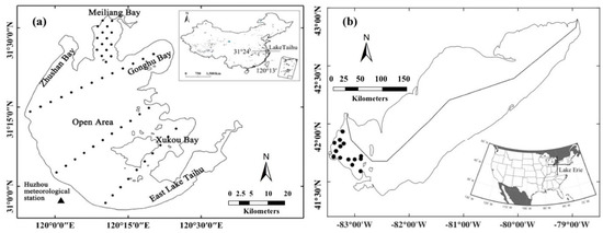
Figure 1.
Station maps of datasets Lake Taihu (a) and Lake Erie (b).
The total absorption coefficient of the bulk water was calculated as the sum of colored dissolved organic matter (CDOM), particulate matter (phytoplankton and tripton), and pure seawater, where the absorption coefficient of pure seawater (aw(λ), m−1) was a constant [27,28]. In this study, the absorption coefficient of CDOM (aCDOM, m−1) and total particle absorption (ap, m−1) were measured using the quantitative filter technique (QFT) following the National Aeronautics and Space Administration (NASA) ocean optical measurement protocol [29]. The procedures are described in Liu et al. [30]. Moreover, the concentrations of suspended particulate matter (SPM, mg/L) and chlorophyll a (including phaeopigments) (Chla, μg/L) were also determined from water samples, and the procedures were described in Liu et al. [30]. In this study, the SPM ranged from ~10.3 to 285.6 mg/L, and the Chla ranged from ~4.9 to 412.7 μg/L. For the absorption coefficients, the a(443) ranged from ~1.4 to 12.5 m−1. A standard Secchi disk with a 30-cm diameter was used to measure ZSD, which ranged from ~0.1 to 0.9 m.
The measurement of Rrs was made following the above-surface approach [31] with an ASD (Analytical Spectral Devices) field spectrometer (Analytical Devices, Inc., Boulder, CO, USA). The radiometer measurements include the total-above surface radiance (Lt), downwelling sky radiance (Lsky) from the reciprocal angle of measuring Lt, and radiance leaving a standard grey card (Lg). The Rrs was then calculated. The equation is shown below.
where ρ is the reflectance of the gray card, and F is the Fresnel reflectance of the air-sea surface, which was approximated as 2.2%. Note that an extra procedure called second-order correction was conducted for calculating Rrs following the procedure of Lee et al. [32]. The measurement of Rrs in our study covers wavelengths up to 1050 nm, so the value of Δ was determined by setting the average of Rrs (950–1000 nm) to be 0 for each station because the absorption coefficient of pure seawater reaches a local maximum (~50 m−1) in this spectral range.
2.1.2. Lake Erie Dataset
One more dataset (Lake Erie, USA) was used to evaluate the QAATI and the ZSD scheme. The measurements (Rrs, a(λ), and ZSD) were collected in western Lake Erie (Figure 1b), and the data were downloaded from the SeaWiFS Bio-optical Archive and Storage System (SeaBASS). A total of 14 sites was included in this dataset, where ZSD values are generally less than 2 m (0.4–1.7 m) with a(443) ranging from ~0.2 to 3.9 m−1.
Above-surface radiance measurements were taken with the Field Spec Pro™ VNIR-NIR1 portable spectrometer system from ASD. The Rrs values were derived following Equation (1).
2.1.3. Satellite Dataset
Another dataset (SAT) was further used to validate the ZSD derived from MERIS. This dataset includes 74 MERIS images and 85 matchups between MERIS Rrs and in-situ ZSD measurements. A total of 74 Level 1 (L1) MERIS images of Lake Taihu from 2003 to 2011 were downloaded from the European Space Agency (ESA) Earth Online (http://earth.esa.int/). The images were then processed using BEAM 5.0 software for geometric referencing and smile correction. There are three plug-in processors provided by the BEAM 5.0 for atmospheric correction of MERIS level 1 data, namely Case-2 Regional Processer (C2R), Boreal Lakes Processor (BOR), and Eutrophic Lakes Processor (EUL). Both C2R and BOR processors were not developed for use in highly eutrophic lake waters [33,34]. Therefore, the atmospheric correction was performed by the artificial neural network scheme included in the EUL processor. Furthermore, a Phycocyanin index (PCI) [35] was used to eliminate the pixels with thick Microcystis bloom. A total of 85 matchups (time difference less than one day) between satellite data and the in-situ ZSD were obtained, where the in-situ ZSD were collected during six field surveys (see Table 2).
Table 2.
Sampling date, number of samples, and distribution of concurrent sampling sites with MERIS for six cruises in the SAT dataset.
To understand the impact of wind speed on the variation of ZSD, the long-term wind speed data of Lake Taihu from 2003 to 2011 were downloaded from the China Meteorological Data Sharing Service System (http://data.cma.cn/). The wind data were collected at the site of Huzhou meteorological station (30°52′ N, 120°3′ E) beside Lake Taihu. The wind data were recorded every 5 min. The daily-averaged wind speed was calculated from all available wind speed data on that day, and the monthly-averaged data were then calculated from the daily-averaged wind speed.
2.1.4. Accuracy Assessment
The performance of an algorithm was quantified based on the mean absolute percentage difference (MAPD), which is defined below.
where x is the evaluated variable, and n is the number of data points.
2.2. Semi-Analytical ZSD Scheme
Based on a new law of contrast reduction, Lee et al. [16] proposed an innovative theoretical model to infer ZSD. Unlike the classical model [12,13] that primarily relies on the beam attenuation coefficient, this model only relies on Kd within the spectral transparent window, and a simplified equation is shown below.
where Min(Kd(λ)) represents the minimum Kd for wavelengths between 443 nm and 665 nm, is the Rrs value that corresponds to the wavelength with the minimum Kd, and is the contrast threshold of the human eye in radiance reflectance and is treated as a constant (0.013 sr−1). Thus, the estimate of ZSD from remote sensing primarily depends on Kd(λ), which can be calculated following the Kd model of Lee et al. [18] from a(λ) and bb(λ). In the ZSD scheme of Lee et al. [18], the values of a(λ) and bb(λ) were retrieved from Rrs with QAA_v6.
In order to obtain accurate estimates of ZSD in turbid inland water, it is critical to have accurate estimation of IOPs from Rrs, but the challenge is that the QAA_v6 and other QAA tuned versions [23,25,26] have difficulty in providing reliable IOPs in such water, which subsequently yields ZSD with high uncertainties (see Section 3.1.1). To extend the applicability of QAA, we provide a revised version described in Section 3.1.2.
3. Results
3.1. QAA Modification and Validation
3.1.1. Evaluation of Current IOPs Estimation Approaches for Turbid Waters
Some efforts have been made to extend the original QAA to retrieve IOPs in turbid waters. For instance, Le et al. [23] attempted to improve the QAA in Meiliang Bay in Lake Taihu by shifting the reference wavelength from the red region to near-infrared (called QAA.Le hereafter). Huang et al. [26] developed a regional QAA (QAA.PY) in the turbid Poyang Lake based on hydro light simulations. Moreover, Yang et al. [25] proposed a revised QAA (QAA.Turbid) for turbid waters by assuming that the optical properties of the near-infrared bands were dominated by the absorption of pure water. Using the entire LT (both LT-A and LT-B) dataset and the Lake Erie dataset, the above three algorithms along with QAA_v6 (two difference reference wavelengths 670 and 710 nm were used separately) were evaluated, in order to understand their performance in turbid inland waters. This comparison of algorithms is intended to (a) characterize the performance of the many revised QAAs in turbid waters, and (b) use ZSD data as an independent data source to measure the performance of these algorithms.
Figure 2 shows histograms of the ratio of the estimated a(λ) (λ = 413, 443, 490, 510, 560, 620, and 665 nm) to in-situ measurements. For the entire LT dataset, the three algorithms (QAA_v6-670, QAA_v6-710, and QAA.Turbid) systematically underestimated the a values with a mean ratio of ~0.6. For the regional algorithms (QAA.Le and QAA.PY), although the mean ratio was relatively closer to 1 (~0.9) than the previous three algorithms, there were still some data points with extremely high ratios (>2) indicating overestimated a values. Similarly, when the above algorithms were evaluated with the other independent dataset (Erie), the absorption coefficients derived from all five algorithms were significantly overestimated with the MAPD ranging from 95.3% to 244.1% (Figure 2a–e).
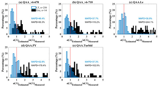
Figure 2.
Evaluation of current IOPs approach for turbid waters for estimating a(λ) (seven wavebands were included in this figure, where λ = 413, 443, 490, 510, 560, 620, and 665 nm) with LT and Erie datasets, respectively.
Furthermore, to understand the uncertainties of derived ZSD with the IOPs estimated from the above QAA algorithms, a comparison of derived ZSD and in-situ measurements is shown in Figure 3. For the entire LT dataset, systematical overestimations were obtained for the algorithms QAA_v6-670 and QAA_v6-710, but underestimated ZSD for the algorithms QAA.Le and QAA.PY (Figure 3a–d). For the Erie dataset, the ZSD derived by all above algorithms were significantly underestimated with the MAPD ranging from 35% to 62% (Figure 3), which is consistent with the systematical overestimation of IOPs (Figure 2a–e). Separately, the QAA. Turbid shows better performance in estimating ZSD than the other four algorithms with a MAPD of 29% and a determination coefficient (r2) of 0.65 for the entire LT dataset (Figure 3e), but for the dataset Erie, the ZSD was systematically underestimated with a MAPD of 39% (Figure 3e).
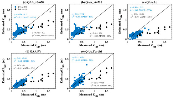
Figure 3.
Evaluation of ZSD for turbid waters for estimation of a(λ) (seven wavebands were included in this figure, where λ = 413, 443, 490, 510, 560, 620, and 665 nm) with LT and Erie datasets, respectively.
3.1.2. Modification of QAA for Highly Turbid Waters
The QAA [36] estimates IOPs (a and bb) in seven steps: two are analytical, three are semi-analytical, and two are empirical (QAA_v6, http://ioccg.org/resources/software/). In oceanic waters, the two empirical steps (Step 2 and 4) are considered of second-order importance because their range of variation and influence on the final output were relatively low. However, the optical properties of turbid inland waters are more complex than oceanic waters and can dramatically change even within small spatial scales. Thus, it is important and necessary to provide reliable relationships for these two steps (Step 2 and 4) in the QAA. In this study, the empirical relationships (Step 2 and 4) are revised with the field measurements collected in Lake Taihu (LT-A dataset, n = 150), and this updated QAA is termed as QAATI herein.
In Step 2, we proposed a new relationship between the absorption coefficient at a reference wavelength (a(λ0)) and Rrs at 560, 665, and 780 nm, which are aimed at applications of MERIS measurements. A key difference of QAATI compared with previous algorithms is the use of 780 nm, which reflects that (1) aw dominates the total absorption coefficient at this wavelength, and (2) the Rrs(780) value of these waters varies in a large range, from 0.002 to 0.025 sr−1, mainly due to large variations in SPM (Figure 4b). Additionally, the usage of 665 nm is considered for less turbid waters. The 560 nm was employed as the reference wavelength (Figure 4a) to reflect the significantly high correlation between a(560) and the Rrs ratios of the above wavelengths (see Figure 5).
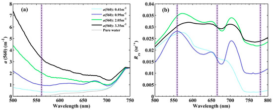
Figure 4.
Examples of (a) a(560) and corresponding (b) Rrs spectrum at different locations.
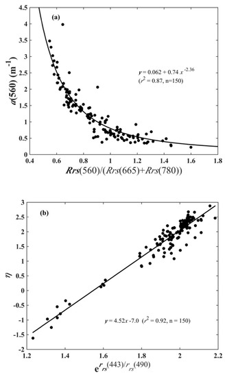
Figure 5.
Empirical models for a(560) (a) and η (b).
Figure 5a shows an excellent relationship between a(560) and Rrs(560)/(Rrs(665) + Rrs(780)), with r2 equal to 0.87. Therefore, a three-band model (Figure 5a) was proposed to estimate a(560), which is shown below.
where 0.062 (m−1) is the absorption coefficient of pure seawater at 560 nm.
It is necessary to know the power coefficient (η) of bbp(λ) (Step 4 of QAA) in all semi-analytical algorithms [21,36,37], and, here, values of η were first derived from the measured Rrs(λ) and a(λ). Specifically, bbp(λ) can be calculated from the following equation.
where u(λ) is the ratio of bb to (a + bb), which can be easily calculated from rrs(λ) (Lee et al., 2002). bbw(λ) is the spectrum of the backscattering coefficient of pure seawater and considered to be a constant [38]. After bbp(λ) is known, η is calculated by linearly fitting the logarithm of bbp(λ) between 400 and 650 nm.
After values of η are known, we used a similar empirical model in QAA_v6 to estimate η but with rrs at 443 nm and 490 nm, and Step 4 of QAATI is written as the equation below (see Figure 5b).
3.1.3. Validation of the QAATI Model: LT_B Dataset and Erie Dataset
To validate the QAATI model, we compared the retrieved a with the measured a at the MERIS bands of 413, 443, 490, 510, 560, 620, and 665 nm using the LT-B dataset. It was found that the estimated and measured a(λ) agree with each other very well (Figure 6), where the r2 is 0.93, and the MAPD is 15.3%.
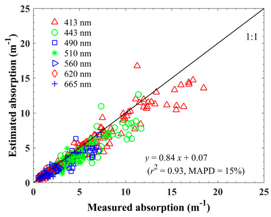
Figure 6.
Comparing the modeled and the measured a(λ) at MERIS bands using the validation (LT-B) dataset.
Furthermore, with the Rrs in the dataset from Lake Erie, the a(λ) was also derived by the QAATI. Figure 7 shows a comparison of measured a(λ) with those derived from Rrs. The r2 is 0.85 with a MAPD as 39.7% (see Figure 7), which suggests very consistent a(λ) between measurements and retrievals. As with Lake Taihu, Lake Erie is also an eutrophic turbid lake, but its optical properties differ significantly from those in Lake Taihu, where the optical properties are highly influenced by rivers and rich terrestrial input from nearby factories [39]. Even so, QAATI performed very well for these two lakes on two different continents, which suggests strongly applicability of QAATI in other similar turbid lakes.
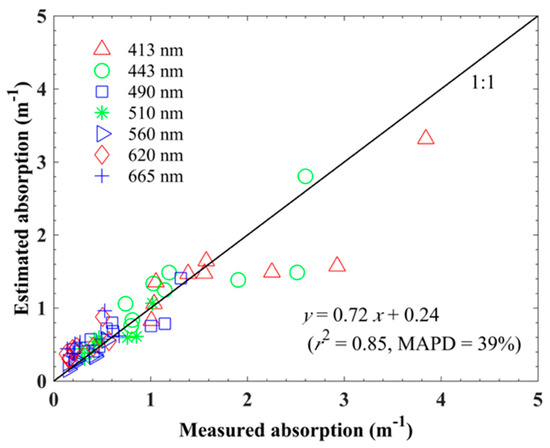
Figure 7.
Comparing the estimated and the measured a(λ) at MERIS bands using the Lake Erie dataset.
3.2. Evaluation of the New ZSD Scheme
3.2.1. LT-A and LT-B Datasets
The new ZSD scheme was first evaluated with the LT-A and LT-B datasets. Figure 8 shows a comparison of the derived ZSD with in-situ measurements, where the derived ZSD match well with the measured ZSD (r2 > 0.65 and MAPD < 25%), even though the ZSD values varied within a very narrow range of ~0.1 to 0.9 m. Considering that both in-situ ZSD measurements and derivation from Rrs have errors/uncertainties, these results suggest a very good performance of the new ZSD scheme for application in such highly turbid lake waters.
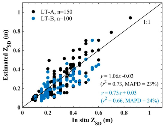
Figure 8.
Comparison of estimated ZSD with in-situ measurements in LT-A and LT-B datasets.
3.2.2. Erie Dataset
The new ZSD scheme was further applied to the Lake Erie dataset (ZSD in a range of 0.4–1.7 m). As shown in Figure 9, an excellent agreement was also found between the estimated ZSD and in-situ measurements (r2 = 0.79, MAPD = 18.6%), where the slope of the regression line is close to 1 and the intercept is close to 0. These results further demonstrated very good performance of the innovative ZSD scheme across a range from clear to turbid waters.
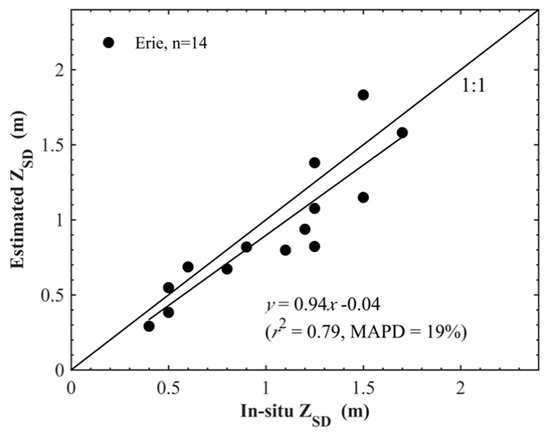
Figure 9.
Comparison of estimated and in-situ ZSD with the Erie dataset.
3.2.3. SAT Dataset
To validate the applicability of the new ZSD scheme to MERIS measurements, the scheme was applied to 74 MERIS images to obtain the spatial distribution of ZSD in Lake Taihu. A total of 85 matchups were obtained with the ZSD ranging from ~0.15 to 1.0 m. A comparison between the satellite-derived ZSD and in-situ measurements is shown in Figure 10. Statistically, the r2 value from a linear regression analysis between the estimated and measured ZSD values is 0.73, and the MAPD is 37% (Figure 10). In the previous study of Doron et al. [12], several ZSD algorithms were evaluated using coincident satellite reflectance and in-situ measurements from both oceanic and coastal waters. It was found that the MAPD between MERIS-derived ZSD and in-situ measurements ranged from 60% to 140%. Comparatively, the ZSD scheme in this study showed much better performance when it is applied to MERIS images, especially for turbid waters.
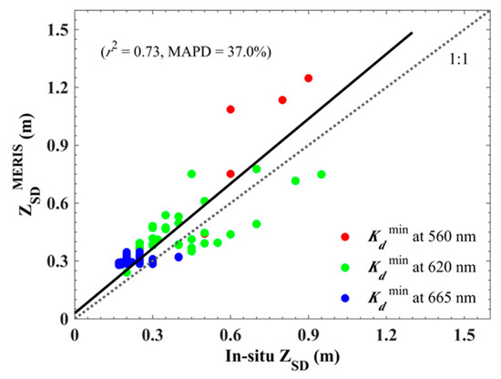
Figure 10.
Comparison between in-situ and MERIS-derived ZSD, where the color denotes the wavelength of minimum Kd.
3.3. Temporal Variation of Water Clarity from MERIS Measurements: Lake Taihu as an Example
3.3.1. Phenological Distribution of ZSD from the MERIS Images
The monthly climatology of ZSD was produced from the MERIS-estimated ZSD data from 2003 to 2011, as shown in Figure 11 and Figure 12. The monthly average ZSD of the entire lake ranged from ~0.24 m to 0.74 m, with a mean of 0.49 m. These values confirmed that Lake Taihu is highly turbid or opaque. Strong seasonal variability in ZSD exists across the entire lake. The monthly mean ZSD of the entire lake is relatively low from December to March, which ranges from 0.24 to 0.30 m with an average of 0.27 m. January exhibited the lowest mean ZSD throughout the year (0.24 m). In April and May, the monthly mean ZSD greatly increased to 0.41 and 0.58 m, respectively. ZSD remained relatively high from June to September, with an average of 0.70 m, and it began to decrease in October and November, with values of 0.56 and 0.41 m, respectively. Possible explanations for these patterns are discussed below.
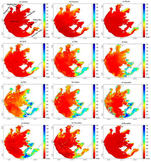
Figure 11.
Phenological distribution of ZSD in Lake Taihu, calculated from all valid pixels of the 74 selected MERIS images using QAATI.
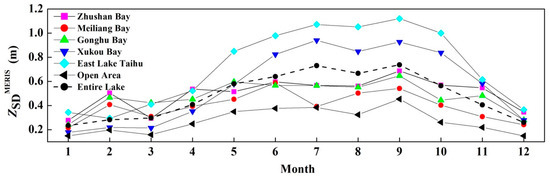
Figure 12.
Phenological variation of ZSD in each region of Lake Taihu.
In terms of the spatial distribution, the ZSD values of open areas were lower, while the ZSD values of bays to the east were relatively higher. Monthly changes in ZSD values from 2003 to 2011 were determined for six regions of Lake Taihu (Zhushan Bay, Meiliang Bay, Gonghu Bay, Xukou Bay, East Lake Taihu, and the Open Area). The distribution pattern of ZSD in January, February, March, and December were similar (Figure 11 and Figure 12): the ZSD values were low in each region. From April to June, the ZSD values in Xukou Bay and East Lake Taihu significantly increased from 0.35 to 0.82 m and from 0.52 to 0.98 m, respectively, followed by Meiliang Bay (from 0.39 to 0.59 m), Gonghu Bay (from 0.44 to 0.57 m), the open area (0.25 to 0.38 m), and Zhushan Bay (0.54 to 0.60 m) (Figure 11 and Figure 12). Moreover, the area with high ZSD in East Lake Taihu rapidly expanded during this period (Figure 11). The ZSD values maintained their high levels in each region from July to October. From October to December, the ZSD values in East Lake Taihu and Xukou Bay remarkably decreased from 1.00 m to 0.37 m and from 0.84 m to 0.28 m, respectively. Compared to East Lake Taihu and Xukou Bay, the decreases in ZSD were lower in the other four regions from October to December.
3.3.2. Factors Affecting ZSD in Lake Taihu
Light attenuation in water is controlled in general by four optically important substances: pure water, CDOM, tripton, and phytoplankton [40]. Among these factors, tripton and phytoplankton form SPM. The concentrations of CDOM, tripton, and phytoplankton may vary in different waters or within the same water during different seasons [30,41,42].
Numerous studies have been conducted concerning the controlling factors of the temporal-spatial variations in light attenuation in Lake Taihu. Previous studies revealed that high SPM concentrations dominate the light attenuation in Lake Taihu [43,44]. The temporal-spatial distribution pattern of ZSD in our study is roughly the same as that from SPM in other studies [44]. In Lake Taihu, the SPM dynamics were found to be controlled by three factors: the lake topography, wind-induced sediment resuspension, and the distribution of macrophytes [44].
The water depth is relatively shallower in the bays and deeper in the open areas. The water depth in each region increases in the following order: East Lake Taihu (1.76 ± 0.37 m, average ± standard error), Xukou Bay (1.82 ± 0.50 m), Zhushan Bay (1.97 ± 0.54 m), Gonghu Bay (1.98 ± 0.44 m), Meiliang Bay (2.11 ± 0.63 m), and the open area (2.63 ± 0.38 m). ZSD remained low in each month in regions with deeper depths, such as Meiliang Bay and the open area (Figure 11 and Figure 12). In contrast, ZSD was significantly higher in shallower regions such as Xukou Bay and East Lake Taihu compared to the other regions throughout the year, except for January, February, and March (Figure 11 and Figure 12). Unlike patterns in the ocean where lower ZSD are in the shallow coastal waters because of sediment resuspension and river input, ZSD is found to decrease with the increase of water depth in Lake Taihu. There are two mechanisms to explain this pattern. First, in the littoral zones and lake bays (shallow waters), the wind fetch was shorter than in the open area (deep waters), which decreased the intensity of wind-driven sediment resuspension and resulted in a higher ZSD than in the open area. Second, there are macrophytes distributed in the shallow area of Lake Taihu, which inhabit the resuspension of sediment, and, thereby, increase water transparency. We analyzed the correlations between the monthly average ZSD and mean water depth in each region and found negative correlations in each month, among which the correlations for November and December were most significant (p < 0.05, Supplementary Figure S1).
Zhang et al. [44] found a positive correlation between the daily wind speed and corresponding SPM concentration in 2003 and 2011 (r 2 = 0.69, p < 0.001). Shi et al. found a positive correlation between the diffuse attenuation coefficient of photosynthetically active radiation (Kd(PAR), m−1) and the wind speed [45] (r2 = 0.85, n = 37, p < 0.005). Therefore, we further investigated the correlation between the monthly average ZSD and wind speed in Lake Taihu. All the valid pixels (not covered by cloud and surface scum) over the entire lake within each month were spatially averaged to generate the corresponding ZSD value. The correlation between the monthly average ZSD and wind speed was statistically significant (p < 0.05), which suggests that the wind speed is a major factor for the phenological variations in ZSD in Lake Taihu (Figure 13), as shown by Shang et al. [46] where wind is a major factor for lower clarity in Bohai Sea.
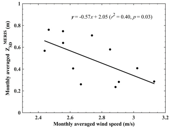
Figure 13.
Linear relationship between monthly averaged wind speed and MERIS-derived ZSD of the entire lake, from 2003 to 2011.
Based on field and remote-sensing observations, macrophytes are abundantly distributed in the littoral regions of East Lake Taihu, Xukou Bay, and Gonghu Bay [43,45]. The growth habits of aquatic vegetation are largely responsible for the monthly variations in ZSD in these regions. From December to the following March, the death and degradation of aquatic vegetation produce lower ZSD values (Figure 11). The growth of aquatic vegetation can improve the underwater light climate by allelopathy and suppress sediment resuspension [44]. Therefore, the area with high ZSD increased in April and May as aquatic vegetation grew. From June to October, the aquatic vegetation reached its peak density and extent [43]. Correspondingly, the highest ZSD values of the year were found in the regions that were dominated by aquatic vegetation during this period (Figure 11).
4. Discussion
4.1. Algorithm Uncertainties
Even if we assume that the in-situ Rrs measurements were completely error-free, multiple sources of uncertainty still affect the accuracy of the final ZSD value. In the new ZSD scheme, the uncertainty of derived ZSD mainly come from a(λ0) and η. According to a systematic study of the sources of uncertainties in IOP products from the QAA, the a(λ0) modeling errors for waters with high absorption coefficients have a larger effect than the η modeling errors on the a(λ) estimation [47]. In our study, we attempted to minimize the uncertainties that are introduced from these two parameters by refining the corresponding steps in QAA. In this step (Step 4), the values of η were derived from a combination of Rrs and a, where a was calculated from ap and aCDOM. Thus, the uncertainties of measured ap and aCDOM as well as those from measured Rrs could propagate to the estimated η. The ap in this study was quantified by utilizing the standard transmittance/reflectance (T-R) method by using the integrating sphere, and the uncertainty for this measurement procedure was found to be ~10% [48]. The detection limit of Ultraviolet (UV) spectrophotometers for the measurement of aCDOM was ~0.0001 absorbance units (equal to ~0.005 m−1 in absorption coefficients) [30]. The uncertainty of this measurement could be relatively low, considering the high aCDOM in eutrophic inland waters (generally greater than ~0.2 m−1 in violet and blue bands).
The power coefficient of bbp, η, is sensitive to the shape of the particle size distribution (PSD), according to theoretical calculations and field measurements [49,50,51]. It was found that small particles generally have enhanced backscattering toward shorter wavelengths, whereas larger particles tend to have a flatter backscattering spectrum. In oceanic water, the water optical properties are determined primarily by phytoplankton and related CDOM and degradation products. Previous studies showed a general decrease in η from oligotrophic to eutrophic regimes in oceanic waters, with higher values of η (>2) in oligotrophic waters where smaller phytoplankton dominate and lower values of η (<1) in more eutrophic waters where larger phytoplankton dominate [52]. In oceanic waters, small-sized phytoplankton (e.g., cyanobacteria, prochlorophytes, and chlorophytes) are incapable of growing beyond a particular chlorophyll concentration, with an upper limit imposed possibly from a combination of a bottom-up (nutrient control) and a top-down (grazing) process [53]. Therefore, an increasing trend of phytoplankton cell size with Chla can be observed in oceanic water and could explain the lower η in eutrophic regimes than in oligotrophic regions. However, in the eutrophic freshwaters, cyanobacteria are the most wide-spread algal taxa [54]. Typically, this species is classified as pico-phytoplankton (0.2–2 μm) and is usually characterized by a cell size of <2 μm [55]. In our study, the derived η value (of a highly eutrophic lake) ranged from −1.6 to 2.8 with a mean value of 1.7, because a large number of samples (~34%) used in this study were collected in regions with highly abundant phytoplankton (Chla > 30 μg/L), where the dominant species was cyanobacteria [56]. Thus, these results could explain the higher η values for some data points in this study. Our results are consistent with reports in the literature regarding particle backscattering in turbid eutrophic waters with high Chla concentrations. Ma et al. [57] showed that the η values calculated from the Hydroscat-6 (HOBI Labs, Watsonville, California) measured backscattering coefficients in Lake Taihu and have a mean value of 2.19 (SD = 0.39). A study in the coastal region of Oslo Fjord also showed that algal bloom (when Chla is greater than 2 μg/L) always associates with steep spectral curves [58]. This finding was further supported by a study in tropical water reservoirs in Queensland, Australia [59]. In addition, in a modelling study of five different cultured phytoplankton species, decreasing backscattering toward longer wavelengths was most significant in the case of cyanobacteria [60], and the η showed an increasing trend with the increase of Chla [61].
For the ZSD maps derived from satellite measurements, another uncertainty is potentially associated with floating algae on the surface of the water. The floating algae is prevalent during the summer months in Lake Taihu when the cyanobacterial blooms occur [30,62]. These masses of floating algae inhibit the reflectance signal of the water column from satellite reception, which results in questionable retrieval of ZSD in these areas during periods with heavy algae. However, because cyanobacteria (the dominant bloom species in Lake Taihu) contain phycocyanin (an accessory pigment with a diagnostic absorption peak at ~620 nm), cyanobacterial blooms can be detected with an algorithm that was developed for MERIS called PCI [35]. By applying this simple algorithm, we detected and removed pixels that were greatly influenced by floating algae. This step can avoid error that is introduced by the influence of thick floating algae. However, the ZSD values in bloom areas are typically low (often <0.2 m in observations). Thus, removing these pixels would cause ZSD to be overestimated in such regions during long-term analysis. The influence of cyanobacterial blooms on the retrieval of water color parameters has not been considered in many previous studies of Lake Taihu, such as those that investigated SPM and Kd (PAR) [43,44,63]. Therefore, this step is expected to be helpful for remote sensing in other very eutrophic waters.
4.2. Implications of the Proposed Model
Many studies of the optical properties of coastal and estuarine regions have revealed that significant correlations exist between SPM and ZSD [64,65]. For example, Lake Frisian in the Netherlands is a shallow water lake with a water depth of 1 to 2 m, and its ZSD is mainly influenced by SPM [66]. Shi et al. [43] evaluated the correlation between ZSD and SPM in Lake Taihu based on 2432 in-situ observations and found a relationship of ZSD = 3.07·SPM−0.60 (r2 = 0.73, p < 0.001). The significant correlation between SPM and ZSD demonstrated that the SPM concentration can be obtained from a semi-analytical model in waters where SPM dominates if the quantitative relationship between SPM and ZSD is determined.
The spatial distributions of ZSD in Lake Taihu were different from that of SPM presented in some previous studies, especially during the summer months. In those studies, the SPM exhibited low values in both phytoplankton-dominated turbid regions (such as Meiliang Bay and Zhushan Bay) and in clear regions that were dominated by submerged macrophytes (such as Xukou Bay and East Lake Taihu) when algal blooms occurred during the summer [43,44,67]. Note that there could be misinterpretations of SPM in phytoplankton-dominated regions, where the absorption and scattering signals in the water column are inhibited when the waters are covered by massive floating algal. Therefore, SPM exhibited similar distribution trends in these two different regions. In our study, the regions covered by serious floating algae were removed by applying a PCI index [35]. Thus, we avoided the influence of floating blooms when retrieving ZSD.
5. Conclusions
Using in-situ measurements collected in Lake Taihu and Lake Erie, we found that the revised QAA algorithm for turbid waters (namely QAATI) showed very good performance for the retrieval of IOPs and ZSD. In particular, with QAATI derived IOPs and an innovative ZSD model, the estimated ZSD from Rrs agree very well with measured ZSD, where ZSD varied from ~0.1–1.7 m. Such results indicate that the presented system can provide a reliable estimation of water clarity of turbid inland waters from the measurement of water color. This implication is further supported by matchup studies between MERIS Rrs and in-situ measurements in Lake Taihu, which opens the door to use MERIS and Sentinel-3 OLCI (SENTINEL-3 Ocean and Land Colour Instrument) to study the spatial and temporal variations of water clarity in turbid lake waters.
Specifically, for Lake Taihu, significant climatologic and spatial variations are revealed from a ~10-year time series provided by MERIS. It was found that the variations of water clarity are jointly controlled by the water depth, wind, waves, and aquatic vegetation distribution in Lake Taihu.
Supplementary Materials
The following are available online at https://www.mdpi.com/2072-4292/11/19/2226/s1.
Author Contributions
Conceptualization, X.L., Z.L., and Y.Z. (Yunlin Zhang). Formal analysis, X.L., Y.Z. (Yunlin Zhang), J.L., and Z.S. Investigation, X.L., Y.Z. (Yunlin Zhang), K.S. and Y.Z. (Yongqiang Zhou). Resources, Y.Z. (Yunlin Zhang) and B.Q. Supervision, Z.L. and Y.Z. (Yunlin Zhang). Writing—original draft, X.L. Writing—review & editing, X.L., Z.L., Y.Z. (Yunlin Zhang), J.L., K.S., and Y.Z. (Yongqiang Zhou).
Funding
The National Natural Science Foundation of China (grant 41621002), the Key Research Program of Frontier Sciences of Chinese Academy of Sciences (QYZDB-SSW-DQC016), the Key Program of the Chinese Academy of Sciences (ZDRW-ZS-2017-3-4), the Natural Science for Youth Foundation (41807362), and the Science and Technology Planning Project of Guangdong Province (2017B010118004) jointly funded this study.
Conflicts of Interest
The authors declare no conflict of interest.
References
- Wernand, M. On the history of the Secchi disc. J. Eur. Opt. Soc. Rapid Publ. 2010, 5, 1–6. [Google Scholar]
- Tyler, J.E. The secchi disc. Limnol. Oceanogr. 1968, 13, 1–6. [Google Scholar]
- Sanden, P.; Håkansson, B. Long-term trends in Secchi depth in the Baltic Sea. Limnol. Oceanogr. 1996, 41, 346–351. [Google Scholar] [CrossRef]
- Swift, T.J.; Perez-Losada, J.; Schladow, S.G.; Reuter, J.E.; Jassby, A.D.; Goldman, C.R. Water clarity modeling in Lake Tahoe: Linking suspended matter characteristics to Secchi depth. Aquat. Sci. 2006, 68, 1–15. [Google Scholar] [CrossRef]
- Davies-Colley, R.J.; Smith, D.G. Turbidity suspended sediment, and water clarity: A review. J. Am. Water Resour. As. 2001, 37, 1085–1101. [Google Scholar] [CrossRef]
- Fleming-Lehtinen, V.; Laamanen, M. Long-term changes in Secchi depth and the role of phytoplankton in explaining light attenuation in the Baltic Sea. Estuar. Coast. Shelf Sci. 2012, 102, 1–10. [Google Scholar] [CrossRef]
- Alikas, K.; Kratzer, S. Improved retrieval of Secchi depth for optically-complex waters using remote sensing data. Ecol. Indic. 2017, 77, 218–227. [Google Scholar]
- Giardino, C.; Pepe, M.; Brivio, P.A.; Ghezzi, P.; Zilioli, E. Detecting chlorophyll, Secchi disk depth and surface temperature in a sub-alpine lake using Landsat imagery. Sci. Total Environ. 2001, 268, 19–29. [Google Scholar] [CrossRef] [PubMed]
- Kratzer, S.; Brockmann, C.; Moore, G. Using MERIS full resolution data to monitor coastal waters—A case study from Himmerfjärden, a fjord-like bay in the northwestern Baltic Sea. Remote Sens. Environ. 2008, 112, 2284–2300. [Google Scholar] [CrossRef]
- Zaneveld, J.R.; Pegau, W. Robust underwater visibility parameter. Opt. Express 2003, 11, 2997–3009. [Google Scholar] [CrossRef]
- Aas, E.; Høkedal, J.; Sørensen, K. Secchi depth in the Oslofjord-Skagerrak area: Theory, experiments and relationships to other quantities. Ocean Sci. 2014, 10, 177–199. [Google Scholar] [CrossRef]
- Doron, M.; Babin, M.; Hembise, O.; Mangin, A.; Garnesson, P. Ocean transparency from space: Validation of algorithms estimating Secchi depth using MERIS, MODIS and SeaWiFS data. Remote Sens. Environ. 2011, 115, 2986–3001. [Google Scholar]
- Preisendorfer, R.W. Secchi disk science: Visual optics of natural waters. Limnol. Oceanogr. 1986, 31, 909–926. [Google Scholar]
- He, X.; Pan, D.; Bai, Y.; Wang, T.; Chen, C.-T.A.; Zhu, Q.; Hao, Z.; Gong, F. Recent changes of global ocean transparency observed by SeaWiFS. Cont. Shelf Res. 2017, 143, 159–166. [Google Scholar]
- Binding, C.E.; Greenberg, T.A.; Watson, S.B.; Rastin, S.; Gould, J. Long term water clarity changes in North America’s Great Lakes from multi-sensor satellite observations. Limnol. Oceanogr. 2015, 60, 1976–1995. [Google Scholar]
- Lee, Z.; Shang, S.; Hu, C.; Du, K.; Weidemann, A.; Hou, W.; Lin, J.; Lin, G. Secchi disk depth: A new theory and mechanistic model for underwater visibility. Remote Sens. Environ. 2015, 169, 139–149. [Google Scholar]
- Lee, Z.; Shang, S.; Du, K.; Wei, J. Resolving the long-standing puzzles about the observed Secchi depth relationships. Limnol. Oceanogr. 2018, 63, 2321–2336. [Google Scholar] [CrossRef]
- Lee, Z.; Hu, C.; Shang, S.; Du, K.; Lewis, M.; Arnone, R.; Brewin, R. Penetration of UV-visible solar radiation in the global oceans: Insights from ocean color remote sensing. J. Geophys. Res. Oceans 2013, 118, 4241–4255. [Google Scholar] [CrossRef]
- Loisel, H.; Poteau, A. Inversion of IOP based on Rrs and remotely retrieved Kd. In Remote Sensing of Inherent Optical Properties: Fundamentals, Tests of Algorithms, and Applications; Reports of the Ocean-Colour Coordinating Group, No. 5; Lee, Z.P., Ed.; IOCCG: Dartmouth, NS, Canada, 2006; pp. 35–41. [Google Scholar]
- Lee, Z.; Carder, K.L.; Arnone, R.A. Deriving inherent optical properties from water color: A multiband quasi-analytical algorithm for optically deep waters. Appl. Optics 2002, 41, 5755–5772. [Google Scholar] [CrossRef]
- Maritorena, S.; Siegel, D.A.; Peterson, A.R. Optimization of a semianalytical ocean color model for global-scale applications. Appl. Optics 2002, 41, 2705–2714. [Google Scholar]
- Lee, Z.; Shang, S.; Qi, L.; Yan, J.; Lin, G. A semi-analytical scheme to estimate Secchi-disk depth from Landsat-8 measurements. Remote Sens. Environ. 2016, 177, 101–106. [Google Scholar] [CrossRef]
- Le, C.F.; Li, Y.M.; Zha, Y.; Sun, D.; Yin, B. Validation of a quasi-analytical algorithm for highly turbid eutrophic water of Meiliang Bay in Taihu Lake, China. IEEE Trans. Geosci. Remote Sens. 2009, 47, 2492–2500. [Google Scholar]
- Rodrigues, T.; Alcântara, E.; Watanabe, F.; Imai, N. Retrieval of Secchi disk depth from a reservoir using a semi-analytical scheme. Remote Sens. Environ. 2017, 198, 213–228. [Google Scholar]
- Yang, W.; Matsushita, B.; Chen, J.; Yoshimura, K.; Fukushima, T. Retrieval of Inherent Optical Properties for Turbid Inland Waters From Remote-Sensing Reflectance. IEEE Trans. Geosci. Remote Sens. 2013, 51, 3761–3773. [Google Scholar] [CrossRef]
- Huang, J.; Chen, L.; Chen, X.; Tian, L.; Feng, L.; Yesou, H.; Li, F. Modification and validation of a quasi-analytical algorithm for inherent optical properties in the turbid waters of Poyang Lake, China. J. Appl. Remote Sens. 2014, 8, 083643. [Google Scholar] [CrossRef]
- Pope, R.M.; Fry, E.S. Absorption spectrum (380–700 nm) of pure water. II. Integrating cavity measurements. Appl. Optics 1997, 36, 8710–8723. [Google Scholar]
- Lee, Z.; Wei, J.; Voss, K.; Lewis, M.; Bricaud, A.; Huot, Y. Hyperspectral absorption coefficient of “pure” seawater in the range of 350–550 nm inverted from remote sensing reflectance. Appl. Optics 2015, 54, 546–558. [Google Scholar]
- Mueller, J.L.; Fargion, G.S.; McClain, C.R.; Pegau, S.; Zanefeld, J.; Mitchell, B.G.; Kahru, M.; Wieland, J.; Stramska, M. Ocean Optics Protocols for Satellite Ocean Color Sensor Validation, Revision 4, Volume IV: Inherent Optical Properties: Instruments, Characterizations, Field Measurements and Data Analysis Protocols; NASA: Greenbelt, MD, USA, 2003.
- Liu, X.; Zhang, Y.; Yin, Y.; Wang, M.; Qin, B. Wind and submerged aquatic vegetation influence bio-optical properties in large shallow Lake Taihu, China. J. Geophys. Res. 2013, 118, 713–727. [Google Scholar] [CrossRef]
- Mueller, J.L.; Davis, C.; Arnone, R.; Frouin, R.; Carder, K.; Lee, Z.; Steward, R.; Hooker, S.; Mobley, C.D.; McLean, S. Above-Water Radiance and Remote Sensing Reflectance Measurements and Analysis Protocols; NASA: Greenbelt, MD, USA, 2000; Volume 2, pp. 98–107.
- Lee, Z.; Ahn, Y.-H.; Mobley, C.; Arnone, R. Removal of surface-reflected light for the measurement of remote-sensing reflectance from an above-surface platform. Opt. Express 2010, 18, 26313–26324. [Google Scholar]
- Doerffer, R.; Schiller, H. The MERIS Case 2 water algorithm. Int. J. Remote Sens. 2007, 28, 517–535. [Google Scholar]
- Doerffer, R.; Schiller, H. MERIS Lake Water Project-Lake Water Algorithm for BEAM ATBD; GKSS Research Center: Geesthacht, Germany, 2008. [Google Scholar]
- Qi, L.; Hu, C.; Duan, H.; Cannizzaro, J.; Ma, R. A novel MERIS algorithm to derive cyanobacterial phycocyanin pigment concentrations in a eutrophic lake: Theoretical basis and practical considerations. Remote Sens. Environ. 2014, 154, 298–317. [Google Scholar]
- Lee, Z. Remote Sensing of Inherent Optical Properties: Fundamentals, Tests of Algorithms, and Applications; International Ocean-Colour Coordinating Group: Dartmouth, NS, Canada, 2006; Volume 5. [Google Scholar]
- Hoge, F.E.; Lyon, P.E. Satellite retrieval of inherent optical properties by linear matrix inversion of oceanic radiance models: An analysis of model and radiance measurement errors. J. Geophys. Res. Oceans 1996, 101, 16631–16648. [Google Scholar]
- Morel, A. Optical properties of pure water and pure sea water. In Optical Aspects of Oceanography; Academic Press: New York, NY, USA, 1974; Volume 1, pp. 1–24. [Google Scholar]
- Qin, B. Lake Taihu, China: Dynamics and Environmental Change; Springer Science & Business Media: Dordrecht, The Netherlands, 2008; Volume 87. [Google Scholar]
- Kirk, J.T.O. Light and Photosynthesis in Aquatic Ecosystems, 3rd ed.; Cambridge University Press: Cambridge, UK, 2011. [Google Scholar]
- Babin, M.; Stramski, D.; Ferrari, G.M.; Claustre, H.; Bricaud, A.; Obolensky, G.; Hoepffner, N. Variations in the light absorption coefficients of phytoplankton, nonalgal particles, and dissolved organic matter in coastal waters around Europe. J. Geophys. Res. Oceans 2003, 108. [Google Scholar] [CrossRef]
- Bricaud, A.; Babin, M.; Claustre, H.; Ras, J.; Tièche, F. Light absorption properties and absorption budget of Southeast Pacific waters. J. Geophys. Res. Oceans 2010, 115. [Google Scholar] [CrossRef]
- Shi, K.; Zhang, Y.; Zhu, G.; Liu, X.; Zhou, Y.; Xu, H.; Qin, B.; Liu, G.; Li, Y. Long-term remote monitoring of total suspended matter concentration in Lake Taihu using 250m MODIS-Aqua data. Remote Sens. Environ. 2015, 164, 43–56. [Google Scholar] [CrossRef]
- Zhang, Y.; Shi, K.; Liu, X.; Zhou, Y.; Qin, B. Lake topography and wind waves determining seasonal-spatial dynamics of total suspended matter in turbid Lake Taihu, China: Assessment using long-term high-resolution MERIS Data. PLoS ONE 2014, 9, e98055. [Google Scholar] [CrossRef] [PubMed]
- Qin, B.; Xu, P.; Wu, Q.; Luo, L.; Zhang, Y. Environmental issues of Lake Taihu, China. Hydrobiologia 2007, 581, 3–14. [Google Scholar]
- Shang, S.; Lee, Z.; Lin, G.; Shi, L.; Wei, G.; Li, X. Water clarity in the Bohai Sea during 2003–2014. In Proceedings of the Ocean Sciences Meeting, Honolulu, HI, USA, 20–24 February 2016. [Google Scholar]
- Lee, Z.; Arnone, R.; Hu, C.; Werdell, P.J.; Lubac, B. Uncertainties of optical parameters and their propagations in an analytical ocean color inversion algorithm. Appl. Optics 2010, 49, 369–381. [Google Scholar]
- Röttgers, R.; Gehnke, S. Measurement of light absorption by aquatic particles: Improvement of the quantitative filter technique by use of an integrating sphere approach. Appl. Optics 2012, 51, 1336–1351. [Google Scholar]
- Reynolds, R.A.; Stramski, D.; Mitchell, B.G. A chlorophyll-dependent semianalytical reflectance model derived from field measurements of absorption and backscattering coefficients within the Southern Ocean. J. Geophys. Res. Oceans 2001, 106, 7125–7138. [Google Scholar]
- Twardowski, M.S.; Boss, E.; Macdonald, J.B.; Pegau, W.S.; Barnard, A.H.; Zaneveld, J.R.V. A model for estimating bulk refractive index from the optical backscattering ratio and the implications for understanding particle composition in case I and case II waters. J. Geophys. Res. Oceans 2001, 106, 14129–14142. [Google Scholar]
- Morel, A. AGARD Lecture Series No. 61, Optics of the Sea (Interface and In-water Transmission and Imaging). North Atlantic Treaty Organisation: London, UK, 1973. [Google Scholar]
- Loisel, H.; Nicolas, J.-M.; Sciandra, A.; Stramski, D.; Poteau, A. Spectral dependency of optical backscattering by marine particles from satellite remote sensing of the global ocean. J. Geophys. Res. 2006, 111. [Google Scholar] [CrossRef]
- Chisholm, S.W. Phytoplankton Size. In Primary Productivity and Biogeochemical Cycles in the Sea; Falkowski, P.G., Woodhead, A.D., Eds.; Springer: New York, NY, USA, 1992. [Google Scholar]
- Paerl, H.W.; Fulton, R.S.; Moisander, P.H.; Dyble, J. Harmful freshwater algal blooms, with an emphasis on cyanobacteria. Sci. World J. 2001, 1, 76–113. [Google Scholar]
- Jeffrey, S.; Mantoura, R.; Wright, S. Phytoplankton Pigments in Oceanography: Guidelines to Modern Methods; Unesco Publishing: Paris, France, 1997. [Google Scholar]
- Deng, J.; Qin, B.; Paerl, H.W.; Zhang, Y.; Ma, J.; Chen, Y. Earlier and warmer springs increase cyanobacterial (Microcystis spp.) blooms in subtropical Lake Taihu, China. Freshwater Biol. 2014, 59, 1076–1085. [Google Scholar]
- Ma, R.; Pan, D.; Duan, H.; Song, Q. Absorption and scattering properties of water body in Taihu Lake, China: Backscattering. Int. J. Remote Sens. 2009, 30, 2321–2335. [Google Scholar]
- Aas, E.; Høkedal, J.; Sørensen, K. Spectral backscattering coefficient in coastal waters. Int. J. Remote Sens. 2005, 26, 331–343. [Google Scholar]
- Campbell, G.; Phinn, S.R.; Daniel, P. The specific inherent optical properties of three sub-tropical and tropical water reservoirs in Queensland, Australia. Hydrobiologia 2010, 658, 233–252. [Google Scholar] [CrossRef]
- Metsamaa, L.; Kutser, T.; Strömbeck, N. Recognising cyanobacterial blooms based on their optical signature: A modelling study. Boreal Environ. Res. 2006, 11, 493–506. [Google Scholar]
- Dupouy, C.; Neveux, J.; Dirberg, G.; Rottgers, R.; Tenório, M.; Ouillon, S. Bio-optical properties of the marine cyanobacteria Trichodesmium spp. J. Appl. Remote Sens. 2008, 2, 023503. [Google Scholar] [CrossRef]
- Qin, B.; Zhu, G.; Gao, G.; Zhang, Y.; Li, W.; Paerl, H.W.; Carmichael, W.W. A drinking water crisis in Lake Taihu, China: Linkage to climatic variability and lake management. Environ. Manag. 2010, 45, 105–112. [Google Scholar] [CrossRef]
- Shi, K.; Zhang, Y.; Liu, X.; Wang, M.; Qin, B. Remote sensing of diffuse attenuation coefficient of photosynthetically active radiation in Lake Taihu using MERIS data. Remote Sens. Environ. 2014, 140, 365–377. [Google Scholar] [CrossRef]
- Liu, J.; Sun, D.; Zhang, Y.; Li, Y. Pre-classification improves relationships between water clarity, light attenuation, and suspended particulates in turbid inland waters. Hydrobiologia 2013, 711, 71–86. [Google Scholar] [CrossRef]
- Pavelsky, T.M.; Smith, L.C. Remote sensing of suspended sediment concentration, flow velocity, and lake recharge in the Peace-Athabasca Delta, Canada. Water Resour. Res. 2009, 45, W11417. [Google Scholar] [CrossRef]
- Dekker, A.G.; Vos, R.J.; Peters, S.W.M. Comparison of remote sensing data, model results and in situ data for total suspended matter (TSM) in the southern Frisian lakes. Sci. Total Environ. 2001, 268, 197–214. [Google Scholar] [CrossRef] [PubMed]
- Ma, R.; Dai, J. Investigation of chlorophyll-a and total suspended matter concentrations using Landsat ETM and field spectral measurement in Taihu Lake, China. Int. J. Remote Sens. 2005, 26, 2779–2795. [Google Scholar]
© 2019 by the authors. Licensee MDPI, Basel, Switzerland. This article is an open access article distributed under the terms and conditions of the Creative Commons Attribution (CC BY) license (http://creativecommons.org/licenses/by/4.0/).