Article

The Impact of Acquisition Date on the Prediction Performance of Topsoil Organic Carbon from Sentinel-2 for Croplands

1
UMR ECOSYS, AgroParisTech, INRA, Université Paris-Saclay, 78850 Thiverval-Grignon, France
2
LISAH, University of Montpellier, INRA-IRD-SupAgro, F-34060 Montpellier, France
3
Indo-French Cell for Water Sciences, IRD, Indian Institute of Science, Bangalore 560012, India
4
INRA, InfoSol Unit, US 1106, 45075 Orléans, France
5
Irstea, University of Montpellier, UMR TETIS, 500 rue François Breton, 34093 Montpellier CEDEX 5, France
*
Author to whom correspondence should be addressed.
Remote Sens. 2019, 11(18), 2143; https://doi.org/10.3390/rs11182143
Submission received: 5 August 2019 / Revised: 7 September 2019 / Accepted: 11 September 2019 / Published: 14 September 2019

Abstract

:
The spatial assessment of soil organic carbon (SOC) is a major environmental challenge, notably for evaluating soil carbon stocks. Recent works have shown the capability of Sentinel-2 optical data to predict SOC content over temperate agroecosystems characterized by annual crops, using a single acquisition date. Considering a Sentinel-2 time series, this work intends to analyze the impact of acquisition date, and related weather and soil surface conditions on the prediction performance of topsoil SOC content (plough layer). A Sentinel-2 time-series was gathered, comprised of the dates corresponding to both the maximum of bare soil coverage and minimum of cloud coverage. Cross-validated partial least squares regression (PLSR) models were constructed between soil reflectance image spectra, and SOC content analyzed from 329 top soil samples collected over the study area. Cross-validation R2 ranged from 0.005 to 0.58, root mean square error from 5.86 to 3.02 g·kg−1 and residual prediction deviation values from 1.0 to 1.5 (without unit), according to date. The main factors influencing these differences were soil roughness, in conjunction with soil moisture, and the cloud and cloud shadow cover of the entire tile. The best performing dates were spring dates characterized by both lowest soil surface roughness and moisture content. Normalized difference vegetation index (NDVI) values below 0.35 did not influence prediction performance. This consolidates the previous results obtained during single date acquisitions and offers wider perspectives for the further use of Sentinel-2 into multidate mosaics for digital soil mapping.

1. Introduction

Soils contain the largest terrestrial pool of organic carbon [1,2,3]. A relatively small increase in the soil organic carbon (SOC) stocks could, therefore, play an important role in limiting the net flux of greenhouse gases towards the atmosphere and mitigating climate change. SOC is also a major component of soil fertility and resilience [4,5], and increasing SOC content may help climate change adaptation and increase food security, especially in soils having low SOC contents. The societal need for monitoring SOC content has been expressed through the 4p1000 initiative [1,2,3], particularly for topsoil, which is directly impacted by tillage practices [4] and receives the most organic inputs. More widely, the various effects that agricultural practices have on SOC changes still need to be appraised [5], which requires updating and monitoring their status and changes in space and time.
The standard method for SOC content measurement consists of collecting soil samples in the field and then preparing 2 mm-sieved air-dried soil samples for their analysis according to standard laboratory determination: it is both time-consuming and expensive. Yet SOC content assessment must be carried out at spatial scales useful for management and for decisions by stakeholders and decision-makers; namely, those at the scale of local, regional, and national or even continental territories. However, until now there is no efficient and straightforward way of monitoring topsoil organic carbon content at such scales. Because soil reflectance in visible near infrared and short wave infrared (Vis-NIR-SWIR, 0.4–2.5 µm) is strongly influenced by SOC and some other soil compounds, such as clay minerals, calcium carbonate and iron oxides, empirical spectral models relating soil reflectance spectra to spectrally-influent properties have been successfully built; e.g., [6,7]. However, this was mostly done under controlled lab conditions (e.g., [6]) and over limited spatial coverages or soil sampling densities. Few studies attempted to spectrally predict SOC contents from Vis-NIR-SWIR image spectra at a regional scale covering tens to some hundreds of km2: they relied either on airborne hyperspectral images [8,9,10], or on satellite hyperspectral HYPERION data [11,12,13], or even on multispectral satellite data of the former generation, such as SPOT-4 and SPOT-5 [14]. The key issue regarding whatever airborne acquisition is concerned, is that they are very expensive and not widely available, even more so at regular time intervals, while the above-mentioned satellite images are also not numerous. Moreover, hyperspectral satellite HYPERION has a low signal-to-noise ratio, while multispectral SPOT satellite sensors have low spectral diversity and resolution, limiting prediction performances.
The new generation Sentinel-2 satellites (S2) launched in 2015 (S2A) and then 2017 (S2B), provide time series with frequent revisit every 5 days, which is very promising for the purpose of updating spatial information on SOC content. Indeed, recent works have shown the relevance of the MultiSpectral Instruments (MSIs) aboard Sentinel-2 satellites to predict SOC content over temperate agroecosystems characterized by annual crops in the Czech Republic [15], Luxemburg, Belgium, Germany [16], and France [17]. The MSI has more spectral bands (13) than previous multispectral satellite sensors, covering the Vis-NIR-SWIR spectral range. S2 data are imaged from space over large areas with a 290 km-swath width, at a spatial resolution of either 10 m (bands 2, 3, 4, 8) or 20 m (bands 5, 6, 7, 8A, 11 and 12), which is sufficient for soil surveying.
In detail however, the prediction performance of these studies, as distinguished with cross-validation residual prediction deviation (RPDcv), varied from 1.0 to 1.8 [15,16,17]. Because of crop rotation, the soil areal fraction that is available for the mapping of topsoil properties from remote sensing imagery varies with acquisition date. Furthermore, soil surface conditions change across the available bare soil areas, particularly in terms of soil moisture and roughness according to tillage operations [18]. The spectral models of SOC content prediction assume that soil organic matter influences the reflectance of bare soil, and such influence operates along the Vis-NIR-SWIR range without unique absorption peaks. Therefore, any factor that disturbs the reflectance spectrum may disturb prediction from this spectrum. Spectral disturbance can be due to: (i) other spectrally influent soil compounds, such as iron, calcium carbonate, coarse fragments [17], water [19,20,21], the presence of a partial vegetation cover [22,23] and crop residues on surface [24,25]; (ii) soil surface morphometry (roughness) that generates differential effects of light [26,27,28]; and (iii) an atmospheric disturbance of the at-field reflectance signal [29,30], varying with season, clouds, sun azimuth and elevation. None of the recent works have investigated the impact that acquisition date may have on prediction performance for SOC content. Gomez et al. [31] showed that several single-date S2 data acquired over a same study area may provide different performances of soil texture prediction, but they did not investigate the reasons for these differences. This is the purpose of the present study, considering an area where encouraging performance was previously obtained from a single spring date of March, for the Versailles Plain [17]: are there optimal dates for predicting topsoil SOC and what are the main factors disturbing the SOC prediction?

2. Materials and Methods

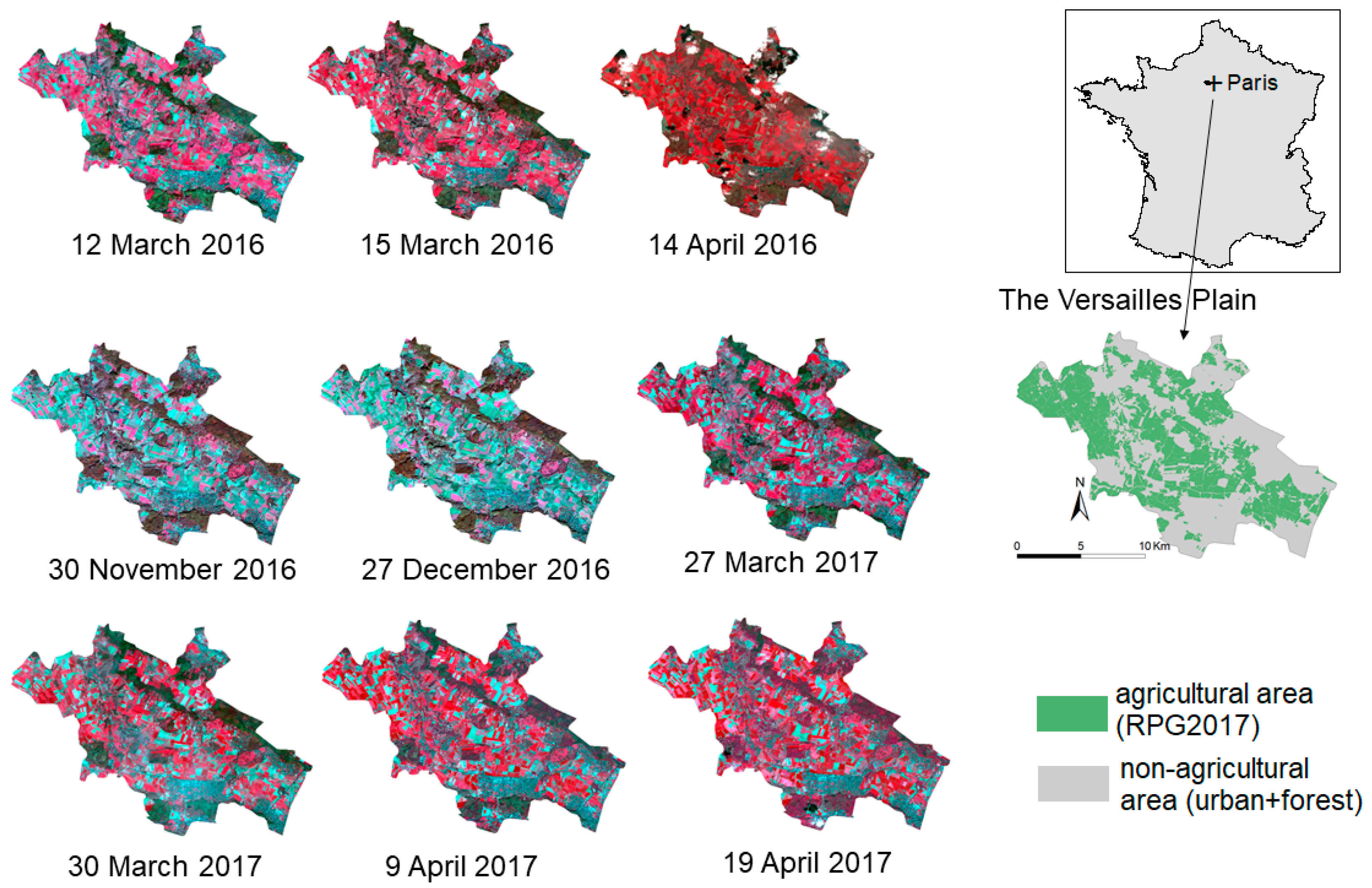
2.1. Study Area: The Versailles Plain

The Versailles Plain, or ‘Plaine de Versailles,’ located west of Paris (North of France, 48°46′–48°56′ N; 1°50′–2°07′ E)) is NW–SE oriented in the view of the esplanade of the Palace of Versailles and covers a total extent of 221 km2, of which about half undergoes intensive annual crop cultivation (Figure 1). It is characterized by a semi-oceanic climate with an average rainfall of 570 mm/year and an average annual temperature of 11.3 °C (INRA meteorological station of Thiverval-Grignon, 1987–2016). The main crop rotations in the area involve winter wheat, winter rapeseed, winter and spring barley, and maize on occasion [32]. Given the crop rotations, bare soil can be observed in the area only in spring and from the middle of autumn to the beginning of winter, while the soil is covered either by crop residues or green vegetation in the remaining periods. As cultivation practices are mainly conventional, with early winter ploughing applied at least one year out of every three, it can be assumed that topsoil SOC is homogenized by ploughing. Landforms are either flat or gently sloping, and structured into a lower limestone plateau at ~120 m elevation in the center and an upper millstone clay plateau at ~170 m elevation along the northern and southern edges of the area. Quaternary loessic deposits and loessic colluvium left a mark everywhere, particularly on plateaus, where haplic or glossic luvisols developed according to the FAO classification (World Reference Base (WRB) [33]) [17,34]. Arenic cambisols developed from the Fontainebleau acid sands across the largely forested upper plateau flanks, while calcaric cambisols derived from limestone in the lower plateau flanks, where colluvial surficial formations are also observed. Along the lower slopes and at the valley bottoms, stagnic colluvic cambisols originated from marls, alluvio-colluvial materials or chalk. The highest SOC values are found in the valley bottoms, followed by lower slopes, then the lower plateaus, while the lowest contents are found for the upper plateaus, and then on the upper plateau flanks [35].

2.2. Sentinel-2 Time Series

For the periods corresponding to a maximum coverage of bare soil, being between 1 March to 30 April in 2016 and 2017, and then between 1 November to 31 December in 2016, a Sentinel-2 time-series of the tile T31UDQ was downloaded from the Muscate platform of the French land data center, called Theia (https://www.theia-land.fr/). In level-2A processing at 10 or 20 meter resolution (bands: 2, 3, 4, 5, 6, 7, 8, 8A, 11 and 12; Table 1), the images were stacked with 10 m resolution. Because the platform discards those images having a cloud cover higher than 90%, and as S2B images were not available yet in April 2017, the series was composed of 13 dates from S2A only instead of the 36 expected dates for S2A. Two dates were very close (12 and 15 March 2016) because at the higher latitudes one can have two observations every 5 days for one S2 satellite due to the higher intersection between two neighboring orbits when approaching poles [24] (Table 2, Figure 1). For each date, ten atmospherically corrected bands with corrections of slope effects were provided, together with a so-called “geophysical mask” (“masque géophysique” or MG2) enabling one to remove clouds and topographical shadows [30].
The images were acquired in near nadir viewing conditions (Table 2) and differed in terms of cloud and shadow cover, which ranged from null to near to 85.5% within the entire tile, and from null to nearly 100% at the very location of the study area. Therefore, four more images had to be discarded from the time series because of their too high cloud cover and shadow coverage: 22 March, 1 April and 7 December 2016, and 29 April 2017.
In order to consider cropland soil only, urban and forest pixels were masked using Land Parcel Registry maps [17]. Cropland pixels assumed to be vegetated, i.e., those with normalized difference vegetation index (NDVI) values exceeding an expert-calibrated threshold, were masked. The NDVI was retrieved using bands of 842 nm and 665 nm. The threshold value of 0.35 was previously used for the date of 12 March 2016 [17] while that of 0.27 was selected as the best trade-off for getting the largest bare soil area while reducing the effects of sparse vegetation on the national scale [36]. In this article, the effects of such thresholding will be compared in §3.3, but the threshold of 0.35 will be used, as it enables to keep a larger number of soil samples, without a significant decrease in prediction performance. Actually, the NDVI threshold of 0.27 suggested the removal of four to 48 samples, compared to 0.35.

2.3. Soil Samples

We used 329 topsoil samples, collected from 2010 to 2017 for the purposes of earlier studies [10,14,17,37,38]. All samples were composed of roughly 10 sub-samples collected to a depth of 8 cm from random locations within a 2.7 × 2.7 m square area centered at the sampling plot, as recorded at its center using a Trimble Pathfinder®Power (Sunnyvale, USA) Differential Global Positioning System (DGPS) of 50 cm precision [18]. Topsoil samples were bulked and air-dried. They were then gently crushed and sieved to 2 mm prior to conventional soil property determinations [39]. Amongst the total number of 329 available soil sample locations, a number of them were vegetated at each date and the available number of the remaining bare soil samples varied between dates (Table 3), never reaching the total of 329. Some bare samples were common to three, four or five dates, and only four were common to all dates.
The SOC content ranged between 6 to 8 and 32 to 36 g·kg−1 (mean 14–16 g·kg−1; standard deviation ~5 g·kg−1) (Table 3). SOC content distribution was slightly positively skewed, whatever date, and was similar between dates, with slightly higher quartiles and mean values for images of the spring 2016.

2.4. Information on Disturbing Factors According to Date

2.4.1. Time-Series of Soil Roughness Maps

In order to assess the temporal changes in soil surface roughness, we used vector maps of soil roughness produced during a previous study over the same area [41] for the five following dates: 27 November and 27 December 2016, and 27 March, 8 April and 20 April 2017. The time difference from the S2 dates was either null (27 December and 27 March), or 1 day (8 and 20 April) and reached a maximum of 3 days only (27 November). Soil roughness was estimated from 10 m radar Sentinel-1 (S1) images according to an approach relying on neural networks trained and validated using large simulated datasets generated from the radar backscattering “integral equation model” (IEM), considering the range of soil moisture and surface roughness encountered in agricultural agroecosystems [42]. Soil roughness, as expressed through the root mean square surface height (Hrms) or standard deviation of the surface height, was validated for the Versailles Plain with a root mean squared error (RMSE) of about 0.80 cm for the spring dates of 2017 [41]. Vector maps, which provide an average value of the estimated soil roughness at each bare field, were intersected with the point shapefile of soil sample locations.

2.4.2. Soil Moisture Measurements and Soil Moisture Index

Topsoil volumetric soil moisture was monitored daily along the whole considered time series at the Integrated Carbon Observation System (ICOS, https://www.icos-ri.eu) ecosystem site FR-Gri, located in the middle of the study area [43]; i.e., within the soilscape unit of the lower limestone plateau mainly characterized by haplic or truncated luvisols. It was averaged for a 0–10 cm depth by four CS650 (Campbell Scientific, Logan, USA) soil water content reflectometers. The ICOS site was vegetated with wheat at the beginning of stem elongation in March–April 2016, and then with oilseed rape in winter 2016 (~15 cm high) and in spring 2017 (60 to 170 cm high). Though not measured on bare soil, the soil moisture from the ICOS site provided information on the major temporal changes in volumetric soil moisture along the observed period.
In addition, soil moisture was determined gravimetrically [44,45] at bare soil locations, coinciding with soil sample locations for the images of 30 March (14 locations) and 19 April (13 locations) 2017. The measurements were performed on 528 cm3 cylinders of the superficial soil horizon that were sampled at between 0 and 8 cm of depth. In analogy to the procedure used by Gao [46] for building the so-called ‘normalized soil water index,’ a relationship was searched for between these measurements and a number of indices involving two or three MSI bands. Based on the bands maximizing differences in reflectance values, the following soil moisture index named ‘S2WI’ was adopted:
S 2 W I = ρ ( 865   n m ) ρ ( 1610   n m ) ρ ( 2190   n m ) ρ ( 865   n m ) + ρ ( 1610   n m ) + ρ ( 2190   n m )
where ρ is surface reflectance (%).
Along the available time series, S2WI values were computed for the samples located within the soilscape unit to which the ICOS site belongs, in order to compare its temporal change with the monitored soil moisture between 0 and 10 cm of depth of the ICOS site.

2.5. Spectral Models of SOC Content Prediction

The partial least squares regression (PLSR) method was chosen to construct prediction models based on bare soil samples drawn at each date. As a matter of fact, it has been widely used in literature for quantitative remote sensing (e.g., [6,7,8,9,10,11,12,13,14,15,16,17]), and therefore, enables comparing our results to those obtained by other authors, particularly for Sentinel-2 [15,16,17]. The PLSR method relates two data matrices, the matrix of explanatory variables X (here the soil reflectance spectra) and the matrix of the dependent variable Y (here the SOC content), through a linear multivariate model; additionally, modelling the structures of X and Y [47,48]. The PLSR approach enables one to analyze data based on several noisy collinear features, and extracts orthogonal or latent predictor variables accounting for variation in the dependent variable Y.
PLSR SOC prediction models were constructed from image reflectance spectra with 10 selected spectral bands (Table 1). As neither log transform nor spectra centering improved prediction performances for several of the considered dates, raw reflectance spectra were used. The optimal number of latent variables was determined from the prediction residual error sum of squares (PRESS). Because we focused on comparing performance levels between dates rather than on carrying out external validation assessments, a leave-one-out cross-validation procedure was applied [48,49]. The quality of model fit was evaluated from the root mean squared error of cross-validation (RMSECV), from the coefficient of the determination of cross-validation (Rcv2) and from the residual prediction deviation (RPD); i.e., the ratio between the standard deviation of the calibration dataset to the RMSECV. PLSR models were used in R version 3.2.1 (R Development Core Team, 2015) employing the “pls” package [50].

3. Results

The performance of SOC content predictions were first analyzed according to acquisition date, then in relation to possible disturbing factors: acquisition condition (§3.2); the presence of vegetation not sufficiently discarded, according to the NDVI cut-off (§3.3); surface roughness (§3.4); and topsoil moisture (§3.5).

3.1. Variations in Prediction Performance According to Date

Performance of SOC content predictions varied according to date, being intermediate (RPD ≥ 1.4) for three spring dates only, and for none of the autumn-winter dates (Table 4). The best models relied on five or six latent variables.
It is noticeable that some models relying on a substantial number of samples (>140) were not performing better than others, suggesting that the large sample size on which they relied did not compensate for possible disturbing factors (30 November 2016, 27 December 2016 and 30 March 2017). Our approach did not intend to elucidate the physical processes of spectral disturbance but rather to exhibit a hierarchy of known disturbing factors. The text below will review, amongst these possible disturbing factors, those varying temporally (atmosphere, vegetation cover, roughness and water).
One must mention, that for each of the three dates affected by the presence of clouds or shadows (14 April and 27 December 2016 and 30 March 2017), some samples were removed by means of the geophysical mask (MG2 notation in Table 4). However, this did not or only slightly for 30 March 2017, improve the performance model. Moreover, two dates very close (12 and 15 March 2016) relied on a similar dataset but resulted in different performance. This requires a closer examination of acquisition conditions.

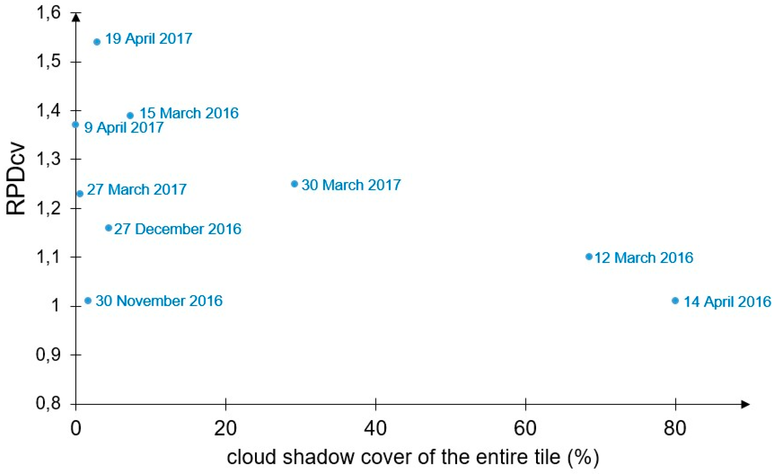
3.2. The Influence of Acquisition Condition

Amongst the factors of acquisition condition described in Table 2, there was a dichotomy between the images extracted from entire tiles with abundant cloud and cloud shadow cover (>65%), both showing low RPDcv, and the remaining dates showing varying RPD values (Figure 2): even though the study area was not specifically affected by cloud cover on 12 March 2016, the presence of clouds and cloud shadows at the scale of the entire tile, to which atmospheric correction was performed, may explain the bad performance for this date compared to 15 March.
In contrast to sun azimuth, there was a positive correlation between sun elevation and RPDcv. When removing the date of 14 April 2016, the most affected by cloud cover, an exponential relationship was exhibited between RPDcv and sun elevation with R2 of 0.6 (Figure 3). This suggests an overall seasonal trend, in favor of spring images compared to autumn and winter images.

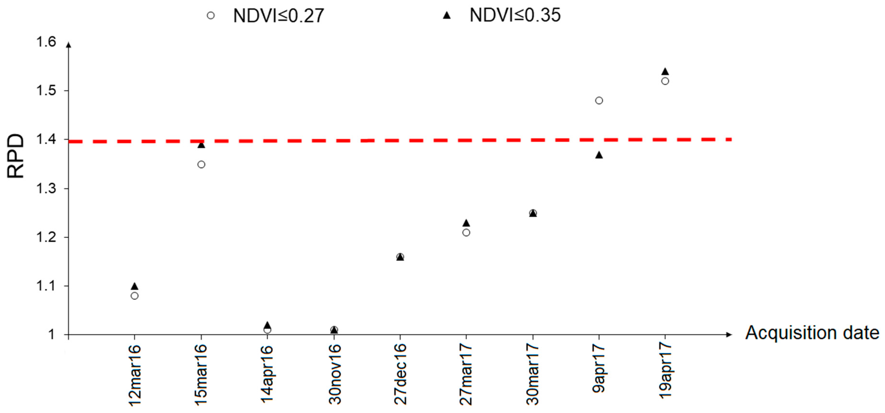
3.3. The Influence of NDVI Threshold

As soil is assumed to be bare below a certain NDVI threshold, one disturbing factor for SOC prediction performance could be the presence of partially covering green vegetation. One might expect that the lower the NDVI threshold, the more exposed soil surface might be. Results in Table 3 were obtained from samples with an NDVI below the 0.35 threshold. However, whatever the NDVI threshold value (0.27 or 0.35), prediction performances were very similar (Figure 4), except on 9 April 2017.
The trade-off between the largest bare soil and the availability of samples for SOC prediction models is thus in favor of keeping more samples, using a higher NDVI.

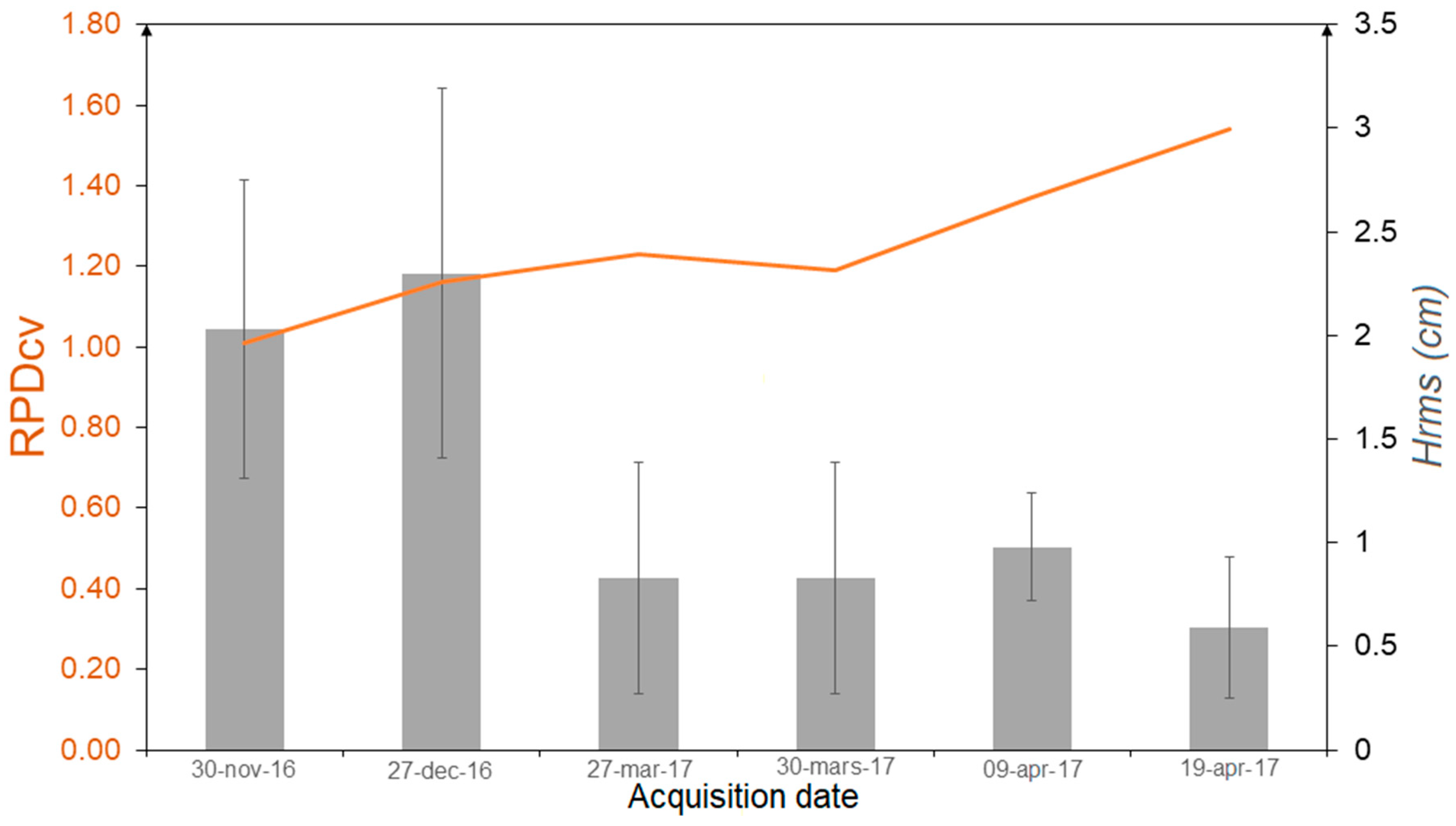
3.4. The Influence of Soil Surface Roughness

Figure 5 displays the histograms of soil roughness, as expressed through Hrms values predicted for each set of soil sample locations one five dates. Winter dates were characterized by pronounced roughness (median ≥2 cm) due to deep ploughing to a soil depth of about 25–30 cm, unlike spring dates (median ≤1 cm), which corresponded to shallow tillage operations (harrowing with vibroshank or rotary cultivator, rolling) for the sowing of spring crops. In addition to shadowing effects, soil surface roughness has directional effects [26], particularly due to tillage practices [27]. As can be expected from its complex spectral effects, soil surface roughness is a major disturbing factor affecting the performance of SOC prediction: the higher the roughness, the lower the prediction performance (Figure 6).

3.5. The Influence of Soil Moisture

The spectral soil moisture index S2WI proved positively related to the measured topsoil moisture in the field (Figure 7). This index was thus calculated for each image, and in the specific case of the soilscape unit represented by the ICOS-Gri ecosystem site, compared to the monitored soil moisture (Figure 8).
Topsoil volumetric moisture of the ICOS-Gri ecosystem site gradually decreased over the 2016–2017 time series, being higher in 2016 compared to Spring 2017 (Figure 8). It was very sensitive to the cumulated rainfall amount of the week preceding each image acquisition as the lowest cumulated rainfall amounts after a week marked clear decreasing trend for 30 November 2016, and for the two dates of April 2017. The spectral S2WI index had negative values for bare soils, ranging from ~−0.5 to 0 (Figure 8). In agreement with the monitored volumetric soil moisture, the mean S2WI values computed for the same soilscape unit as the ICOS-Gri site were much higher in 2016 (above −0.2) than for the Spring 2017 (below −0.3). The S2WI index is therefore useful for characterizing topsoil moisture, at least for separating between very moist and very dry soils along a time series.
SOC prediction performance, as expressed through RPDcv, tended to decrease along with higher S2WI values; i.e., higher soil moisture (Figure 9). However, such a correlation held true for the SU4 soilscape containing ICOS-Gri only, and could not be extrapolated for the other soilscape units, due to the lack of soil moisture information.

4. Discussion

SOC prediction performance varies with acquisition date. It depends on a number of factors, amongst which soil roughness exhibited the most significant influence for this study. This is in compliance with previous studies, based on reflectance field spectra and field roughness measurements, that have shown the negative influence of soil surface roughness on SOC prediction performance [28,51]. From the seasonal relationship between SOC prediction performance and soil surface roughness, we can infer, or at least confirm, the best periods for predicting SOC from S2 images.

4.1. Optimal Dates for Predicting SOC from S2 Images and the Benefit of S2/S1 Synergy

As can be expected from our previous spring studies within the same area [10,14,28], late spring images enabled optimal SOC prediction performances. As a matter of fact, provided low cumulated weekly rainfall before acquisition, soils are mostly smooth and dry in late spring. On the contrary, they are mostly rough and moist in autumn and winter, while the situation is intermediate in early spring.
Regarding the specific influence of soil surface roughness, these trends were highlighted from the synergy between S2 and S1, and particularly, S1-derived surface roughness that was previously assessed at several dates [41]. Bousbih et al [52] have also recently taken advantage of S2/S1 synergy for improving the prediction of soil clay texture, but in order to better target the clayey soils expected to slow drying, their strategy opted for the most humid periods between September and December; they, therefore, used S1-derived soil moisture instead of roughness.

4.2. The Need for Further S1-Derived Soil Moisture Information

Only a weak relationship between soil moisture and SOC prediction performance came through the soil moisture data that were available. Although the averaged S2WI values for the SU4 unit of haplic or truncated luvisols were consistent with the trends of soil moisture variations at the ICOS-Gri ecosystem site, there was no link between soil moisture, as estimated through S2WI, and the overall SOC residuals across all dates (Figure 10). Therefore, the effect of soil moisture on SOC performance prediction remained unclear. Yet, several authors demonstrated the negative effect that increasing soil moisture had on SOC prediction performance, from laboratory spectra [19,20], and also from both laboratory and field-moist spectra [21]. Nevertheless, Rienzi et al. [20] found that SOC prediction from a spectral library could maintain an acceptable quality, even with a varying range of volumetric soil moisture content of between 15% and 25%. As soil moisture measured in the field in spring 2017 ranged throughout that interval and reached even lower values (Figure 7), it might explain the weak relationship observed between SOC prediction performance and soil moisture, at least for spring dates.
A further use of S1 data should enable a more straightforward analysis of soil surface moisture, than the S2WI values did. S2WI values fitted topsoil cylinder measurements moderately (R2 = 0.66) but this was for volumetric soil moisture contents ranging from very low (7%, stony soil) to intermediate (22%) values in spring. Further soil moisture measurements would be needed to validate this relationship for higher soil moisture levels. Moreover, the interpretation of S2WI values must be done with caution for the luvisols prone to hardsetting [53], as illustrated by Figure 8. For the dates of 27 and 30 March 2017—soil might be interpreted as dry according to its S2WI low value (<−0.3) but may be moist under the soil surface’s slaking crust. For this specific effect, both the validity range and slaking effect require further study related to the S2WI. This is the reason why the combined use of a synchronous radar image would probably be useful, not only for this purpose, but also for a more direct assessment of the soil moisture levels across the considered time-series. Currently, two types of algorithm for surface soil moisture (SSM) estimation are considered from Synthetic-Aperture Radar (SAR) data and are particularly well adapted to bare soils pixels. The first type algorithm is the change detection (CD) approach which is applied using multi-temporal SAR images with high revisit time [54,55,56]. The change detection approach supposes that the change in backscattering coefficients between two successive dates is only related to changes in the SSM, while other parameters contributing to SAR backscattering, such as soil roughness and vegetation, remain stable. The second type of algorithm is based on the use of the neural network technique (NN) to estimate the SSM from SAR data [57,58,59]. Paloscia et al. [60] and El Hajj et al. [61] proposed an approach based on the neural NN technique for operational SSM mapping from S1 and S2 images.

4.3. The Assumption of No or Few Crop Residues on the Surface

Crop residues were assumed negligible on the soil surface at the considered dates. As it relies on our observed dataset across eight successive years, such an assumption is robust for spring, while, for winter, it stems from expert knowledge of the agricultural practices that predominate over the study area. Crop residues are mostly found after cereal harvest, which is carried out from late July to early September for the Versailles Plain. A further study dealing with the detection of crop residues along the year, and particularly with the relationship to the key harvest dates of main and intermediate crops [62], has been initiated to verify the assumption of little or no crop residue cover for winter dates.
Intensive crop cultivation implying mechanical conventional tillage today still predominates in the Versailles Plain. With an eventual shift to conservation tillage, our results may no longer be valid, as it would require one to handle the soil surface partially covered with both crop residues and emerging crops. Such a complex surface condition is hardly detectable from S2 and would rather require hyperspectral satellite sensors, such as from the newly launched PRISMA or the forthcoming EnMap, CHIME, SHALOM or HypXim.

4.4. The Influence of the Spatial Level of Atmospheric Correction and Dataset Composition

Across the considered time-series, acquisition conditions as expressed through the cloud and cloud shadow cover of the entire tile and sun elevation proved to be influential on SOC prediction performance. In particular, the specific case of the image acquired on 12 March 2016, for which nearly no cloud occurred at the scale of the study zone, conversely to the entire tile (Figure 1), suggests that the spatial coverage of atmospheric correction does matter and may degrade the accuracy of atmospheric correction and hence SOC prediction performance. As a matter of fact, in our previous study [17], atmospheric correction was parameterized at the scale of the study area, resulting in an intermediate RPDcv for the same image, instead of the poor performance in this study. The specific influence that atmospheric correction processors and processing scales have on SOC predictions’ performances should be studied further for the whole time series.
Moreover, from one date to another, the composition of the dataset varies according to crop development changes. This is why there actually existed no common validation set for the whole series (only four sampling locations). The differences due to spatial arrangement and soil type composition (Table 3) were assumed negligible between dates. Common datasets of 26 and 40 sampling locations were found for only seven or five dates respectively, but were not used, having debatable representativeness.
In further works, it could be interesting to handle a common dataset for model comparison, as well as maximize bare soil coverage, by assessing strategies for mosaicking several images into multidate mosaics [63]. Although performances proved higher for spring, it is noticeable that our dataset contained one winter date and one autumn date only: a number of acquisitions were discarded because of high cloud coverage at these seasons. A further work would consist of handling more winter and autumn dates, and for this purpose, deep learning techniques could be tested for such an extended time series.

5. Conclusions

The choice of acquisition date is crucial for achieving an acceptable SOC prediction performance from S2 images. SOC prediction performance indeed varies with acquisition date. It depends on a number of factors, amongst which soil roughness exhibited the most significant influence in this study. The agricultural operations that influence soil surface roughness need to be taken in to account, along with the agricultural practices leading to crop residues and the main rainfall events. SOC prediction performances proved higher for spring dates with low surface roughness, along with those with no crop residues and no preceding rainfall events. Our study also highlights the benefit of S2/S1 synergy for topsoil property monitoring and opens perspectives for the further use of Sentinel-2 into multidate mosaics for digital soil mapping. Deep learning techniques could also be tested for an extended time series that would contain more winter and autumn dates.

Author Contributions

Conceptualization, E.V., C.G., P.L., T.L. and D.A.; methodology, E.V., C.G. and L.A.; validation, E.V.; resources, N.B., T.L. and B.L; writing—original draft preparation, E.V.; writing—review and editing, all co-authors; project administration, P.L.; funding acquisition, P.L. and E.V.

Funding

This work was supported by CNES, France, and was carried out in the framework of the TOSCA “Cartographie Numérique des Sols (CNS)” program (grant number 3261-3264 CES Theia CartoSols) of the CNES. It also benefited from support from the TOSCA-PLEIADES-CO program (grant number 3249 SENTINEL_PLEIADES-CO) of the CNES.

Acknowledgments

Special thanks to Dalila Hadjar and Dav Ebengo, for technical assistance in the field. D.A. and P.L. are respectively coordinator and collaborator of the Research Consortium GLADSOILMAP, supported by LE STUDIUM Loire Valley Institute for Advanced studies.

Conflicts of Interest

The authors declare no conflict of interest.

References

  1. Minasny, B.; Malone, B.P.; McBratney, A.B.; Angers, D.A.; Arrouays, D.; Chambers, A.; Chaplot, V.; Chen, Z.-S.; Cheng, K.; Das, B.S.; et al. Soil carbon 4 per mille. Geoderma 2017, 292, 59–86. [Google Scholar] [CrossRef]
  2. Arrouays, D.; Horn, R. Soil Carbon—4 per Mille—An introduction. Soil Tillage Res. 2019, 188, 1–2. [Google Scholar] [CrossRef]
  3. Soussana, J.-F.; Lutfalla, S.; Ehrhardt, F.; Rosenstock, T.; Lamanna, C.; Havlík, P.; Richards, M.; Wollenberg, E.L.; Chotte, J.-L.; Torquebiau, E.; et al. Matching policy and science: Rationale for the ‘4 per 1000 - soils for food security and climate’ initiative. Soil Tillage Res. 2019, 188, 3–15. [Google Scholar] [CrossRef]
  4. Balesdent, J.; Chenu, C.; Balabane, M. Relationship of soil organic matter dynamics to physical protection and tillage. Soil Tillage Res. 2000, 53, 215–230. [Google Scholar] [CrossRef]
  5. Chenu, C.; Angers, D.A.; Barré, P.; Derrien, D.; Arrouays, D.; Balesdent, J. Increasing organic stocks in agricultural soils: Knowledge gaps and potential innovations. Soil Tillage Res. 2019, 188, 41–52. [Google Scholar] [CrossRef]
  6. Viscarra Rossel, R.A.; Walvoort, D.J.J.; McBratney, A.B.; Janik, L.J.; Skjemstad, J.O. Visible, near infrared, mid infrared or combined diffuse reflectance spectroscopy for simultaneous assessment of various soil properties. Geoderma 2006, 131, 59–75. [Google Scholar] [CrossRef]
  7. Cécillon, L.; Barthès, B.G.; Gomez, C.; Ertlen, D.; Genot, V.; Hedde, M.; Stevens, A.; Brun, J.J. Assessment and monitoring of soil quality using near-infrared reflectance spectroscopy (NIRS). Eur. J. Soil Sci. 2009, 60, 770–784. [Google Scholar] [CrossRef] [Green Version]
  8. Selige, T.; Böhner, J.; Schmidhalter, U. High resolution topsoil mapping using hyperspectral image and field data in multivariate regression modeling procedures. Geoderma 2006, 136, 235–244. [Google Scholar] [CrossRef]
  9. Stevens, A.; Udelhoven, T.; Denis, A.; Tychon, B.; Lioy, R.; Hoffmann, L.; van Wesemael, B. Measuring soil organic carbon in croplands at regional scale using airborne imaging spectroscopy. Geoderma 2010, 158, 32–45. [Google Scholar] [CrossRef]
  10. Vaudour, E.; Gilliot, J.M.; Bel, L.; Lefevre, J.; Chehdi, K. Regional prediction of soil organic carbon content over temperate croplands using visible near-infrared airborne hyperspectral imagery and synchronous field spectra. Int. J. Appl. Earth Obs. Geoinform. 2016, 49, 24–38. [Google Scholar] [CrossRef]
  11. Gomez, C.; Viscarra Rossel, R.A.; McBratney, A.B. Soil organic carbon prediction by hyperspectral remote sensing and field vis-NIR spectroscopy: An Australian case study. Geoderma 2008, 146, 403–411. [Google Scholar] [CrossRef]
  12. Lu, P.; Wang, L.; Niu, Z.; Li, L.; Zhang, W. Prediction of soil properties using laboratory VIS–NIR spectroscopy and Hyperion imagery. J. Geochem. Explor. 2013, 132, 26–33. [Google Scholar] [CrossRef]
  13. Minu, S.; Shetty, A.; Minasny, B.; Gomez, C. The role of atmospheric correction algorithms in the prediction of soil organic carbon from Hyperion data. Int. J. Remote Sens. 2017, 38, 6435–6456. [Google Scholar] [CrossRef]
  14. Vaudour, E.; Bel, L.; Gilliot, J.M.; Coquet, Y.; Hadjar, D.; Cambier, P.; Michelin, J.; Houot, S. Potential of SPOT Multispectral Satellite Images for Mapping Topsoil Organic Carbon Content over Peri-Urban Croplands. Soil Sci. Soc. Am. J. 2013, 77, 2122. [Google Scholar] [CrossRef]
  15. Gholizadeh, A.; Žižala, D.; Saberioon, M.; Borůvka, L. Soil organic carbon and texture retrieving and mapping using proximal, airborne and Sentinel-2 spectral imaging. Remote Sens. Environ. 2018, 218, 89–103. [Google Scholar] [CrossRef]
  16. Castaldi, F.; Hueni, A.; Chabrillat, S.; Ward, K.; Buttafuoco, G.; Bomans, B.; Vreys, K.; Brell, M.; van Wesemael, B. Evaluating the capability of the Sentinel 2 data for soil organic carbon prediction in croplands. ISPRS J. Photogramm. Remote Sens. 2019, 147, 267–282. [Google Scholar] [CrossRef]
  17. Vaudour, E.; Gomez, C.; Fouad, Y.; Lagacherie, P. Sentinel-2 image capacities to predict common topsoil properties of temperate and Mediterranean agroecosystems. Remote Sens. Environ. 2019, 223, 21–33. [Google Scholar] [CrossRef]
  18. Vaudour, E.; Baghdadi, N.; Gilliot, J.M. Mapping tillage operations over a peri-urban region using combined SPOT4 and ASAR/ENVISAT images. Int. J. Appl. Earth Obs. Geoinform. 2014, 28, 43–59. [Google Scholar] [CrossRef]
  19. Minasny, B.; McBratney, A.B.; Bellon-Maurel, V.; Roger, J.-M.; Gobrecht, A.; Ferrand, L.; Joalland, S. Removing the effect of soil moisture from NIR diffuse reflectance spectra for the prediction of soil organic carbon. Geoderma 2011, 167–168, 118–124. [Google Scholar] [CrossRef]
  20. Rienzi, E.A.; Mijatovic, B.; Mueller, T.G.; Matocha, C.J.; Sikora, F.J.; Castrignanò, A. Prediction of Soil Organic Carbon under Varying Moisture Levels Using Reflectance Spectroscopy. Soil Sci. Soc. Am. J. 2014, 78, 958. [Google Scholar] [CrossRef]
  21. Ackerson, J.P.; Demattê, J.A.M.; Morgan, C.L.S. Predicting clay content on field-moist intact tropical soils using a dried, ground VisNIR library with external parameter orthogonalization. Geoderma 2015, 259–260, 196–204. [Google Scholar] [CrossRef]
  22. Bartholomeus, H.; Kooistra, L.; Stevens, A.; van Leeuwen, M.; van Wesemael, B.; Ben-Dor, E.; Tychon, B. Soil Organic Carbon mapping of partially vegetated agricultural fields with imaging spectroscopy. Int. J. Appl. Earth Obs. Geoinform. 2011, 13, 81–88. [Google Scholar] [CrossRef]
  23. Ouerghemmi, W.; Gomez, C.; Naceur, S.; Lagacherie, P. Applying blind source separation on hyperspectral data for clay content estimation over partially vegetated surfaces. Geoderma 2011, 163, 227–237. [Google Scholar] [CrossRef]
  24. Daughtry, C.S.T.; McMurtrey, J.E.; Chappelle, E.W.; Dulaney, W.P.; Irons, J.R.; Satterwhite, M.B. Potential for Discriminating Crop Residues from Soil by Reflectance and Fluorescence. Agron. J. 1995, 87, 165. [Google Scholar] [CrossRef]
  25. Serbin, G.; Daughtry, C.S.T.; Hunt, E.R.; Brown, D.J.; McCarty, G.W. Effect of Soil Spectral Properties on Remote Sensing of Crop Residue Cover. Soil Sci. Soc. Am. J. 2009, 73, 1545. [Google Scholar] [CrossRef]
  26. Jacquemoud, S.; Baret, F.; Hanocq, J.F. Modeling spectral and bidirectional soil reflectance. Remote Sens. Environ. 1992, 41, 123–132. [Google Scholar] [CrossRef]
  27. Cierniewski, J.; Verbrugghe, M.; Marlewski, A. Effects of farming works on soil surface bidirectional reflectance measurements and modelling. Int. J. Remote Sens. 2002, 23, 1075–1094. [Google Scholar] [CrossRef]
  28. Denis, A.; Stevens, A.; van Wesemael, B.; Udelhoven, T.; Tychon, B. Soil organic carbon assessment by field and airborne spectrometry in bare croplands: Accounting for soil surface roughness. Geoderma 2014, 226–227, 94–102. [Google Scholar] [CrossRef]
  29. Hagolle, O. Directional Effect Correction for Sentinel-2 Composites, Blog “Séries Temporelles”. 2014. Available online: http://www.cesbio.ups-tlse.fr/multitemp/?p=4039 (accessed on 5 August 2019).
  30. Baetens, L.; Desjardins, C.; Hagolle, O. Validation of Copernicus Sentinel-2 Cloud Masks Obtained from MAJA, Sen2Cor, and FMask Processors Using Reference Cloud Masks Generated with a Supervised Active Learning Procedure. Remote Sens. 2019, 11, 433. [Google Scholar] [CrossRef]
  31. Gomez, C.; Dharumarajan, S.; Féret, J.-B.; Lagacherie, P.; Ruiz, L.; Sekhar, M. Use of Sentinel-2 Time-Series Images for Classification and Uncertainty Analysis of Inherent Biophysical Property: Case of Soil Texture Mapping. Remote Sens. 2019, 11, 565. [Google Scholar] [CrossRef]
  32. Vaudour, E.; Noirot-Cosson, P.E.; Membrive, O. Early-season mapping of crops and cultural operations using very high spatial resolution Pléiades images. Int. J. Appl. Earth Obs. Geoinform. 2015, 42, 128–141. [Google Scholar] [CrossRef]
  33. World Reference Base (WRB). World Reference Base for Soil Resources: A Framework for International Classification, Correlation and Communication; Food and Agriculture Organization of the United Nations: Rome, Italy, 2014; 128p. [Google Scholar]
  34. Crahet, M. Soil Map of the Versailles Plain. Scale 1:50,000; Internal Report; Institut National Agronomique Paris-Grignon: Grignon, France, 1992. [Google Scholar]
  35. Zaouche, M.; Bel, L.; Vaudour, E. Geostatistical mapping of topsoil organic carbon and uncertainty assessment in Western Paris croplands (France). Geoderma Reg. 2017, 10, 126–137. [Google Scholar] [CrossRef]
  36. Loiseau, T.; Chen, S.; Mulder, V.L.; Román Dobarco, M.; Richer-de-Forges, A.C.; Lehmann, S.; Bourennane, H.; Saby, N.P.A.; Martin, M.P.; Vaudour, E.; et al. Satellite data integration for soil clay content modelling at a national scale. Int. J. Appl. Earth Obs. Geoinform. 2019, 82, 101905. [Google Scholar] [CrossRef]
  37. Gilliot, J.M.; Vaudour, E.; Michelin, J. Soil surface roughness measurement: A new fully automatic photogrammetric approach applied to agricultural bare fields. Comput. Electron. Agric. 2017, 134, 63–78. [Google Scholar] [CrossRef]
  38. Ebengo, D.M.; Vaudour, E.; Gilliot, J.M.; Hadjar, D.; Baghdadi, N. Potential of combined Sentinel 1/Sentinel 2 images for mapping topsoil organic carbon content over cropland taking into account soil roughness. In Proceedings of the European Geophysical Union General Assembly 2018, Vienna, Austria, 8–13 April 2018. [Google Scholar]
  39. Baize, D.; Jabiol, B. Guide Pour la Description des Sols; Éditions Quae: Paris, France, 2011. [Google Scholar]
  40. Joanes, D.N.; Gill, C.A. Comparing measures of sample skewness and kurtosis. J. R. Stat. Soc. Ser. D 1998, 47, 183–189. [Google Scholar] [CrossRef]
  41. Baghdadi, N.; El Hajj, M.; Choker, M.; Zribi, M.; Bazzi, H.; Vaudour, E.; Gilliot, J.-M.; Ebengo, D. Potential of Sentinel-1 Images for Estimating the Soil Roughness over Bare Agricultural Soils. Water 2018, 10, 131. [Google Scholar] [CrossRef]
  42. Baghdadi, N.; Choker, M.; Zribi, M.; Hajj, M.E.; Paloscia, S.; Verhoest, N.E.C.; Lievens, H.; Baup, F.; Mattia, F. A new empirical model for radar scattering from bare soil surfaces. Remote Sens. 2016, 18, 920. [Google Scholar] [CrossRef]
  43. Loubet, B.; Laville, P.; Lehuger, S.; Larmanou, E.; Fléchard, C.; Mascher, N.; Genermont, S.; Roche, R.; Ferrara, R.M.; Stella, P.; et al. Carbon, nitrogen and Greenhouse gases budgets over a four years crop rotation in northern France. Plant Soil 2011, 343, 109–137. [Google Scholar] [CrossRef]
  44. Gardner, W.H. Water Content. In Methods of Soil Analysis: Part 1—Physical and Mineralogical Methods; SSSA Book Series; Soil Science Society of America, American Society of Agronomy: Madison, WI, USA, 1986; pp. 493–544. ISBN 978-0-89118-864-3. [Google Scholar] [CrossRef]
  45. AFNOR. Soil Quality—Determination of Soil Water Content as a Volume Fraction Using Coring Sleeves—Gravimetric Method—Qualité du Sol; NF EN ISO 11461; AFNOR: Paris, France, 2014. [Google Scholar]
  46. Gao, B. NDWI—A normalized difference water index for remote sensing of vegetation liquid water from space. Remote Sens. Environ. 1996, 58, 257–266. [Google Scholar] [CrossRef]
  47. Geladi, P.; Kowalski, B.R. Partial least-squares regression: A tutorial. Anal. Chim. Acta 1986, 185, 1–17. [Google Scholar] [CrossRef]
  48. Wold, S.; Sjöström, M.; Eriksson, L. PLS-regression: A basic tool of chemometrics. Chemom. Intell. Lab. Syst. 2001, 58, 109–130. [Google Scholar] [CrossRef]
  49. Gomez, C.; Lagacherie, P.; Coulouma, G. Regional predictions of eight common soil properties and their spatial structures from hyperspectral Vis–NIR data. Geoderma 2012, 189, 176–185. [Google Scholar] [CrossRef]
  50. Wehrens, R.; Mevik, B.-H. The pls package: Principal component and partial least squares regression in R. J. Stat. Softw. 2007. [Google Scholar] [CrossRef]
  51. Rodionov, A.; Pätzold, S.; Welp, G.; Pallares, R.C.; Damerow, L.; Amelung, W. Sensing of Soil Organic Carbon Using Visible and Near-Infrared Spectroscopy at Variable Moisture and Surface Roughness. Soil Sci. Soc. Am. J. 2014, 78, 949. [Google Scholar] [CrossRef]
  52. Bousbih, S.; Zribi, M.; Pelletier, C.; Gorrab, A.; Lili-Chabaane, Z.; Baghdadi, N.; Ben Aissa, N.; Mougenot, B. Soil Texture Estimation Using Radar and Optical Data from Sentinel-1 and Sentinel-2. Remote Sens. 2019, 11, 1520. [Google Scholar] [CrossRef]
  53. Bresson, L.M.; Moran, C.J. Structural change induced by wetting and drying in seedbeds of a hardsetting soil with contrasting aggregate size distribution. Eur. J. Soil Sci. 1995, 46, 205–214. [Google Scholar] [CrossRef]
  54. Njoku, E.G.; Jackson, T.J.; Lakshmi, V.; Chan, T.K.; Nghiem, S.V. Soil moisture retrieval from AMSR-E. IEEE Trans. Geosci. Remote Sens. 2003, 41, 215–229. [Google Scholar] [CrossRef]
  55. Kerr, Y.H.; Waldteufel, P.; Wigneron, J.-P.; Delwart, S.; Cabot, F.; Boutin, J.; Escorihuela, M.-J.; Font, J.; Reul, N.; Gruhier, C. The SMOS mission: New tool for monitoring key elements of the global water cycle. Proc. IEEE 2010, 98, 666–687. [Google Scholar] [CrossRef]
  56. Zribi, M.; Kotti, F.; Amri, R.; Wagner, W.; Shabou, M.; Lili-Chabaane, Z.; Baghdadi, N. Soil moisture mapping in a semiarid region, based on ASAR/Wide Swath satellite data. Water Resour. Res. 2014, 50, 823–835. [Google Scholar] [CrossRef] [Green Version]
  57. Baghdadi, N.; Cresson, R.; El Hajj, M.; Ludwig, R.; La Jeunesse, I. Estimation of soil parameters over bare agriculture areas from C-band polarimetric SAR data using neural networks. Hydrol. Earth Syst. Sci. 2012, 16, 1607–1621. [Google Scholar] [CrossRef] [Green Version]
  58. Baghdadi, N.; EL Hajj, M.; Zribi, M.; Fayad, I. Coupling SAR C-Band and Optical Data for Soil Moisture and Leaf Area Index Retrieval Over Irrigated Grasslands. IEEE J. Sel. Top. Appl. Earth Obs. Remote Sens. 2016, 9, 1229–1243. [Google Scholar] [CrossRef]
  59. El Hajj, M.; Baghdadi, N.; Zribi, M.; Belaud, G.; Cheviron, B.; Courault, D.; Charron, F. Soil moisture retrieval over irrigated grassland using X-band SAR data. Remote Sens. Environ. 2016, 176, 202–218. [Google Scholar] [CrossRef] [Green Version]
  60. Paloscia, S.; Pettinato, S.; Santi, E.; Notarnicola, C.; Pasolli, L.; Reppucci, A. Soil moisture mapping using Sentinel-1 images: Algorithm and preliminary validation. Remote Sens. Environ. 2013, 134, 234–248. [Google Scholar] [CrossRef]
  61. El Hajj, M.; Baghdadi, N.; Zribi, M.; Bazzi, H. Synergic use of Sentinel-1 and Sentinel-2 images for operational soil moisture mapping at high spatial resolution over agricultural areas. Remote Sens. 2017, 9, 1292. [Google Scholar] [CrossRef]
  62. Rivas, H.; Delbart, N.; Ottlé, C.; Maignan, F.; Vaudour, E. Monitoring phenology of crops at the parcel scale: Combining high and medium spatial resolution data. Geophys. Res. Abstr. 2019, 21, 1. [Google Scholar]
  63. Vaudour, E.; Gomez, C.; Loiseau, T.; Lagacherie, P.; Arrouays, D. Mosaicking approaches for predicting topsoil organic carbon content from Sentinel-2 time series. In Proceedings of the Food Security and Climate Change: 4 Per 1000 Initiative New Tangible Global Challenges for the Soil, Poitiers, France, 17–20 June 2019. [Google Scholar]
Figure 1. Agricultural area of the Versailles Plain and infrared colored images (RGB = B8, B4 and B3) of the Sentinel-2 time series gathered for this study. RPG2017 (for Registre Parcellaire Graphique) is the Land Parcel Registry map composed of the 2017 crops declared by farmers in the framework of the European Agricultural Policy.
Remotesensing 11 02143 g001
Figure 2. Plot of cross-validation residual prediction deviation (RPDcv) against the cloud and cloud shadow cover of the entire tile.
Remotesensing 11 02143 g002
Figure 3. Plot of RPDcv against sun elevation and regression equation, excluding 14 April 2016.
Remotesensing 11 02143 g003
Figure 4. Influence of an NDVI threshold on residual prediction deviation (RPD).
Remotesensing 11 02143 g004
Figure 5. Histograms of Sentinel-1 (S1)-derived root mean square surface height (Hrms) values obtained from Baghdadi et al. (2018) [31] at the soil sample locations for five dates (red line: median value).
Remotesensing 11 02143 g005
Figure 6. Evolution of prediction performance according to S2 acquisition date and S1-derived soil surface roughness for these dates (the same Hrms value was assigned to 27 and 30 March).
Remotesensing 11 02143 g006
Figure 7. The relationship between the soil moisture index S2WI and the measured topsoil moisture in the field.
Remotesensing 11 02143 g007
Figure 8. Evolution of S2WI according to volumetric soil moisture and soil surface roughness Hrms for the soilscape unit 4, with photographs of soil surface conditions of early and late spring 2017. Error bars for the Hrms refer to the standard deviation of Hrms values for the soil sample locations pertaining soilscape unit 4.
Remotesensing 11 02143 g008
Figure 9. Plot of RPDcv against the mean S2WI for the SU4 soilscape unit equipped at the ICOS-Gri site.
Remotesensing 11 02143 g009
Figure 10. Plot of residuals of SOC prediction (resSOC) against S2WI for all dates.
Remotesensing 11 02143 g010
Table 1. Specifications of a Sentinel-2 MultiSpectral Instrument sensor (in bold characters, bands provided by the Muscate platform used in this work).
Spectral BandSpectral DomainCentral Wavelength (nm)Bandwidth (nm)Spatial Resolution (m)
B1Vis4432060
B2Vis4906510
B3Vis5603510
B4Vis6653010
B5R-edge7051520
B6R-edge7401520
B7R-edge7832020
B8NIR84211510
B8ANIR8652020
B9NIR9452060
B10SWIR13803060
B11SWIR16109020
B12SWIR219018020
Vis, visible; R-edge, red edge; NIR, near infrared; SWIR, shortwave infrared.
Table 2. Main characteristics of the studied scenes (tile TUDQ31): S, spring; A, autumn; W, winter.
SeasonImaging DateTime of Acquisition (U.T GMT)Viewing Incidence Zenith Angle (°)Sun Azimuth (°)Sun Elevation (°)Cloud/Shadow Cover of the Entire Tile (%)Cloud/Shadow Cover of Study Area (%)Date of Soil Roughness Map
S12 March 201610:50:37<5.1160.536.168.60.2none
S15 March 201611:01:57<8.8153.537.87.30none
S14 April 201610:57:23≤8.8163.549.580.046.6none
A30 November 201611:04:18≤8.8172.218.71.71.027 November 2016
W27 December 201610:55:27≤5.0166.916.54.41.027 December 2016
S27 March 201710:50:21≤5.0160.242.00.60.927 March 2017
S30 March 201711:03:34<8.8163.543.729.251.9none
S9 April 201711:05:29≤8.8163.547.3008 April 2017
S19 April 201711:06:01<8.8163.451.22.90.920 April 2017
Table 3. Statistics of soil organic carbon (SOC) contents (g·kg−1) according to dates (normalized difference vegetation index (NDVI) ≤ 0.35).
Imaging DateNumber of SamplesMin1st QuartileMedianMean3rd QuartileMaxStandard DeviationSkewness 1
12 March 2016837.0412.6516.2016.8120.3031.905.230.45
15 March 2016847.0412.6816.9316.3020.5031.905.270.41
14 April 2016867.0412.6216.3016.8820.3531.905.160.42
30 November 20161996.2011.0513.2014.9518.3035.905.130.96
27 December 20161736.2011.1013.2015.1718.3035.905.601.23
27 March 20171478.9211.6014.7015.8418.3035.905.471.28
30 March 20171446.3811.4714.7015.8118.3035.905.551.23
9 April 20171256.3811.4014.2015.0917.9031.904.630.96
19 April 20171226.3811.4014.1515.0817.8831.904.660.97
Whole dataset3296.2011.3014.2015.4218.5035.905.220.96
1 type 3 skewness according to Joanes and Gill [40].
Table 4. Sentinel-2 (S2) prediction performance by date (in bold characters, intermediate performance)—NDVI ≥ 0.35. MG2 denotes the models based on samples not influenced by clouds or shadows according to the MG2 mask.
Imaging DateNumber of SamplesNumber of Latent VariablesRMSECV (g·kg−1)R2CVRPDCV
12 March 20168334.780.161.1
15 March 20168453.790.481.4
14 April 20168635.050.031.0
14 April 2016-MG25415.860.0051.0
30 November 201619935.070.021.0
27 December 201617364.820.261.2
27 December 2016-MG217264.830.251.2
27 March 201714744.450.331.2
30 March 201714464.680.291.2
30 March 2017-MG26755.440.351.3
9 April 201712553.380.461.4
19 April 201712263.020.581.5

