Forward and Backward Visual Fusion Approach to Motion Estimation with High Robustness and Low Cost

Abstract
1. Introduction
1.1. Motivations and Technical Challenges
1.2. Literature Review
1.3. Main Contributions
2. Materials and Methods
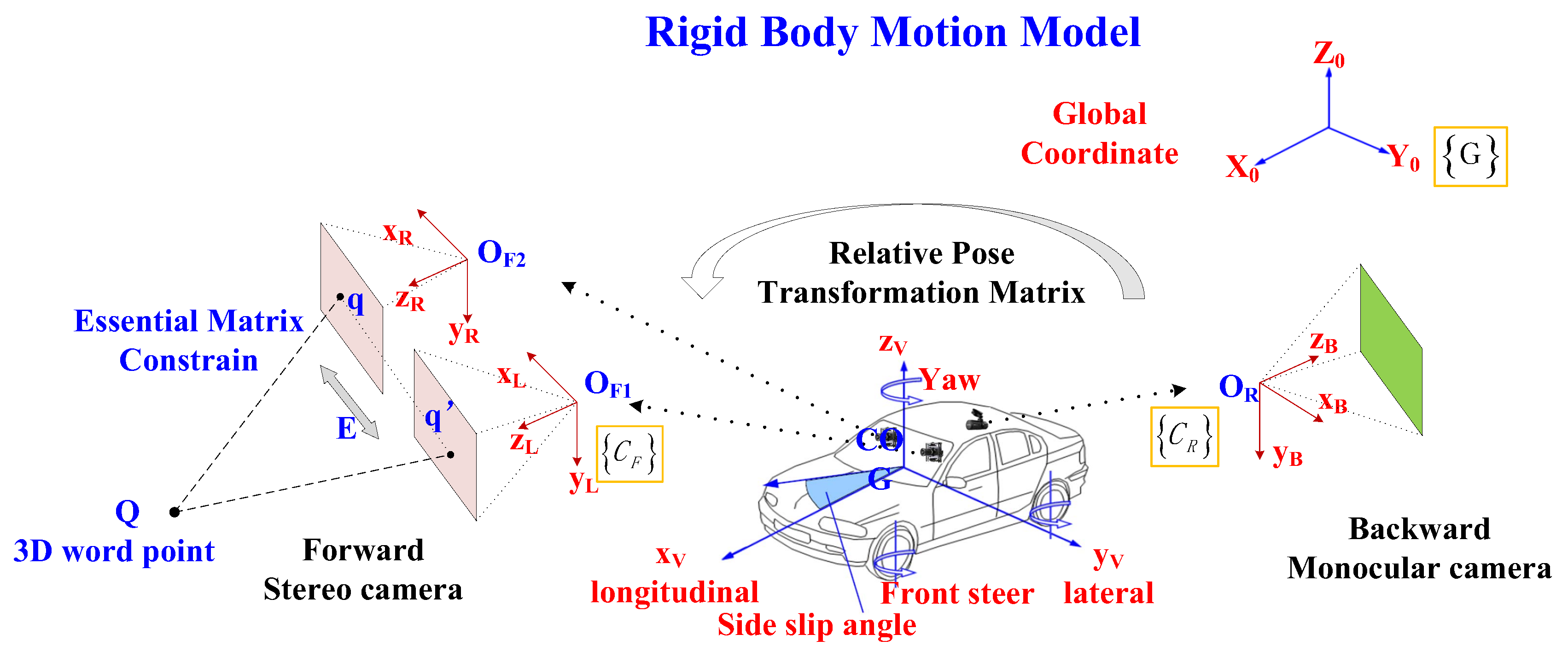
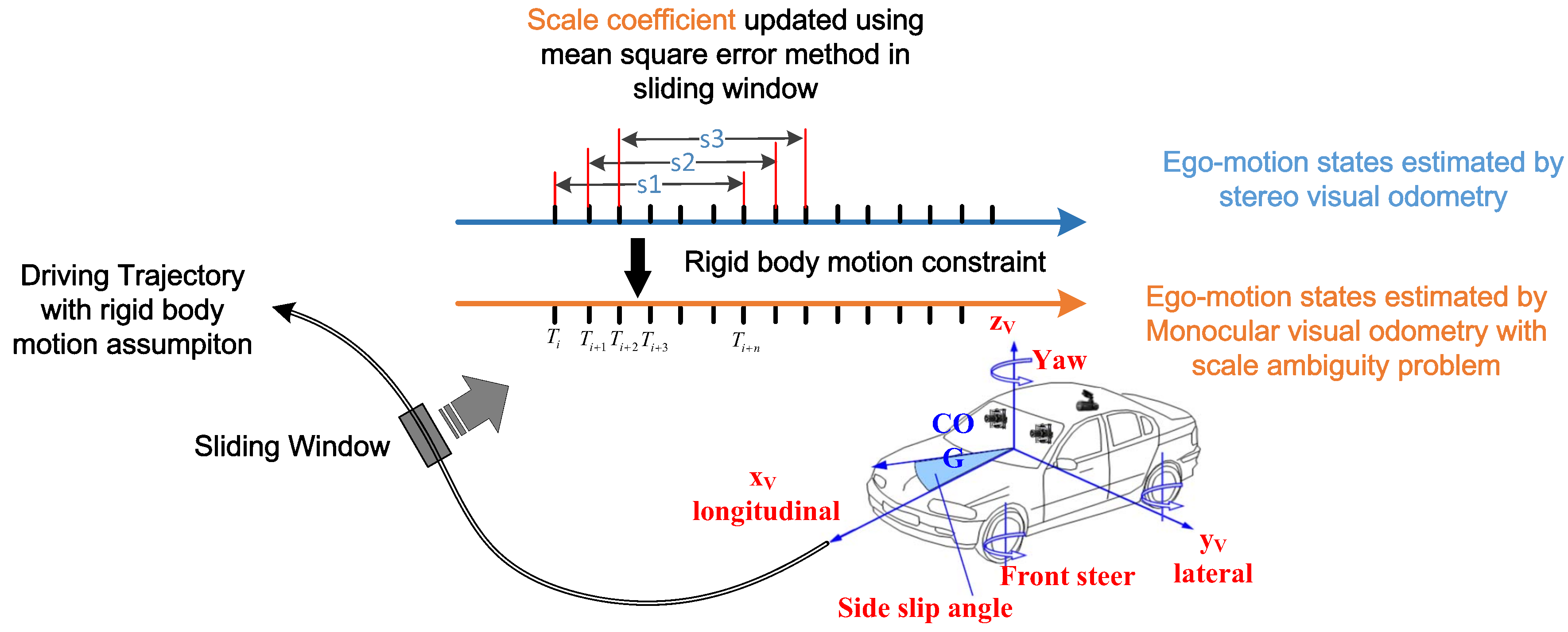
2.1. Assumptions and Coordinate Systems
- We parallel X-O-Y plane of to the horizontal plane. The -axis points opposite to gravity. The -axis points forward of the mobile platform, and the -axis is determined by the right-hand rule.
- Forward camera coordinate system is set originated at the left camera optical center of stereo camera system . The x-axis points to the left, the y-axis points upward, and the z-axis points forward coinciding with the camera principal axis.
- Backward camera coordinate system is originated at the camera optical center of monocular camera system . The x-axis points to the left, the y-axis points upward, and the z-axis points forward coinciding with the camera principal axis.
2.2. Data Association of Forward-Facing and Backward-Facing Cameras
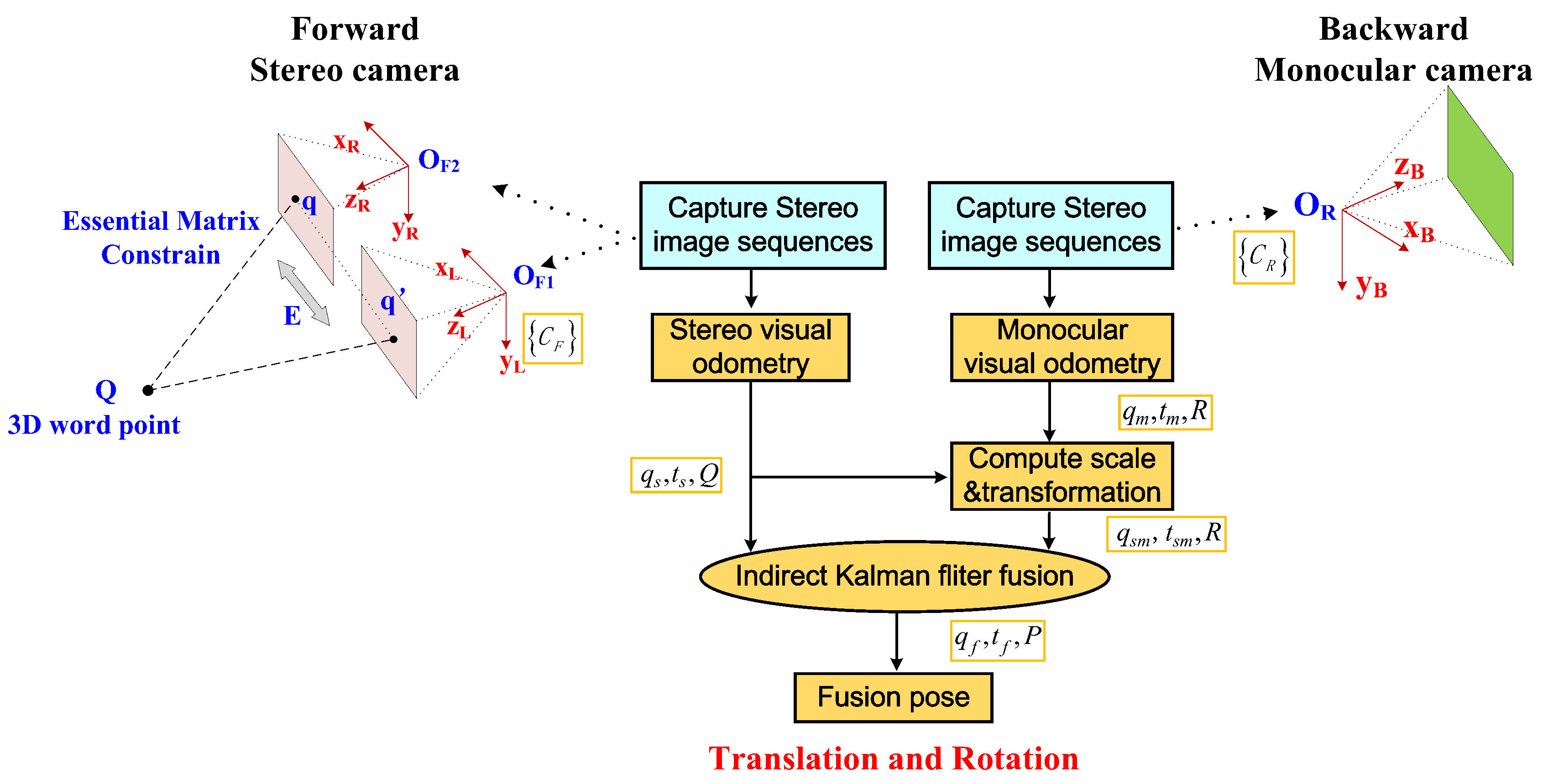
2.3. Loosely Coupled Framework for Trajectory Fusion
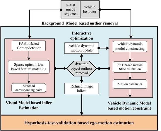
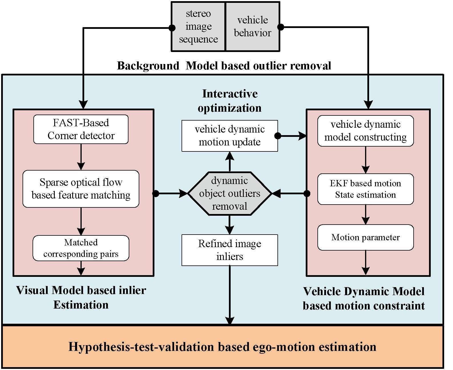
2.4. Basic Visual Odometry Method
2.5. Scale of Monocular Visual Odometry
2.6. Kalman Filter Based Trajectory Fusion
2.6.1. Prediction Equation and Observation Equation
2.6.2. Calculation of Covariance Matrix
2.6.3. Two-Layers Kalman Filter Based Trajectory Fusion
3. Results
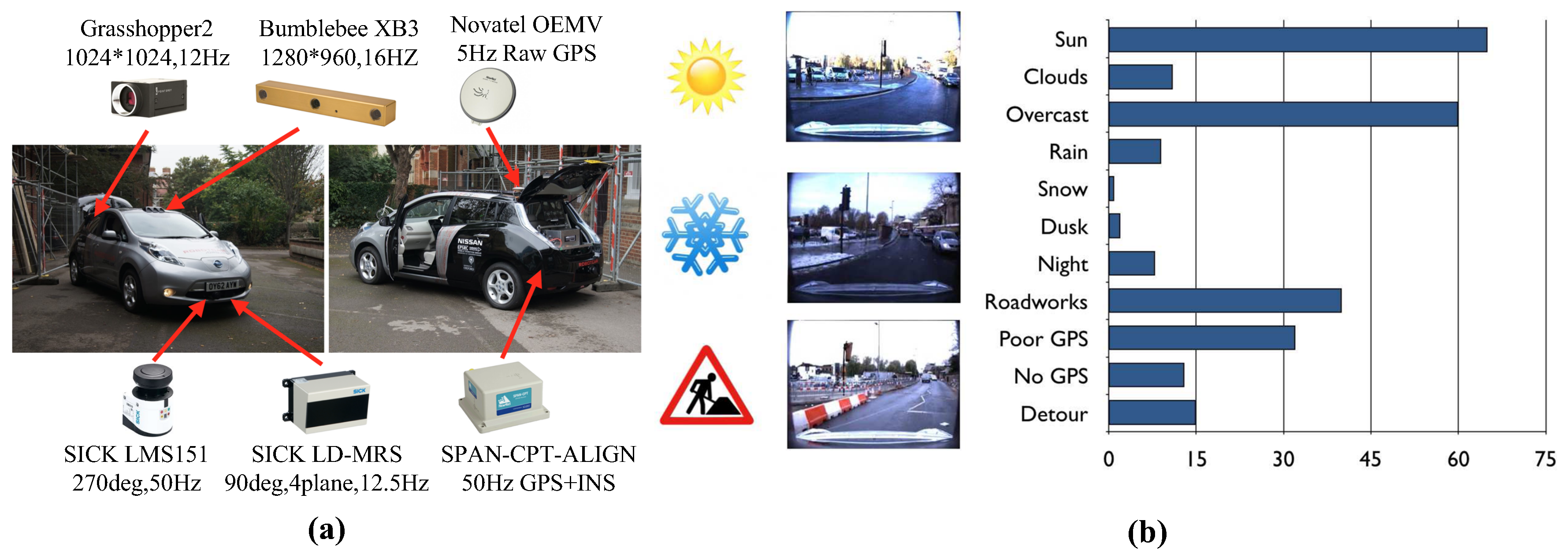
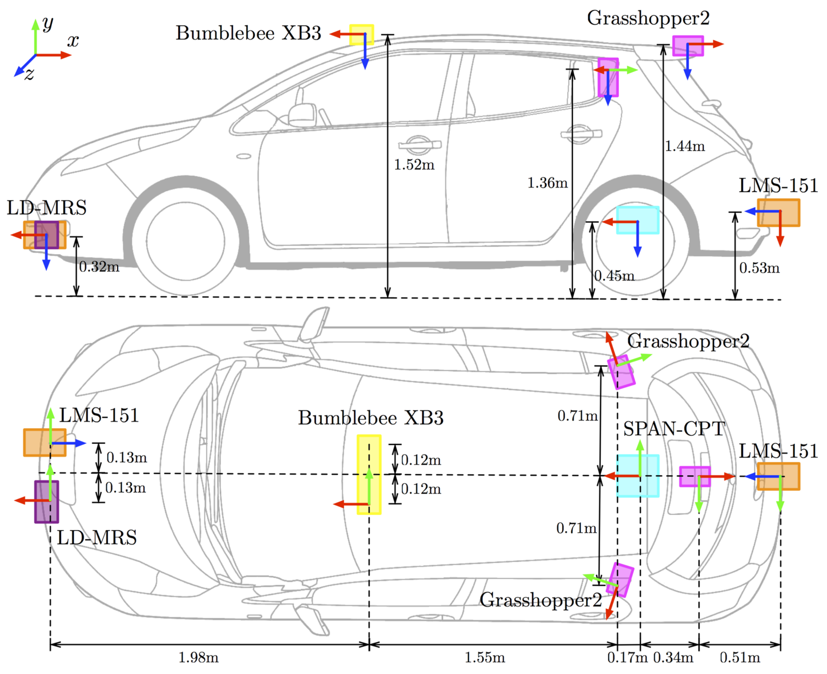
3.1. Oxford RobotCar Dataset
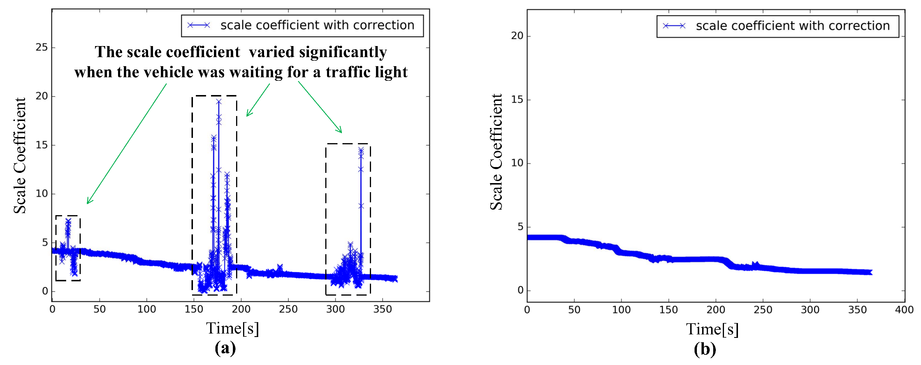
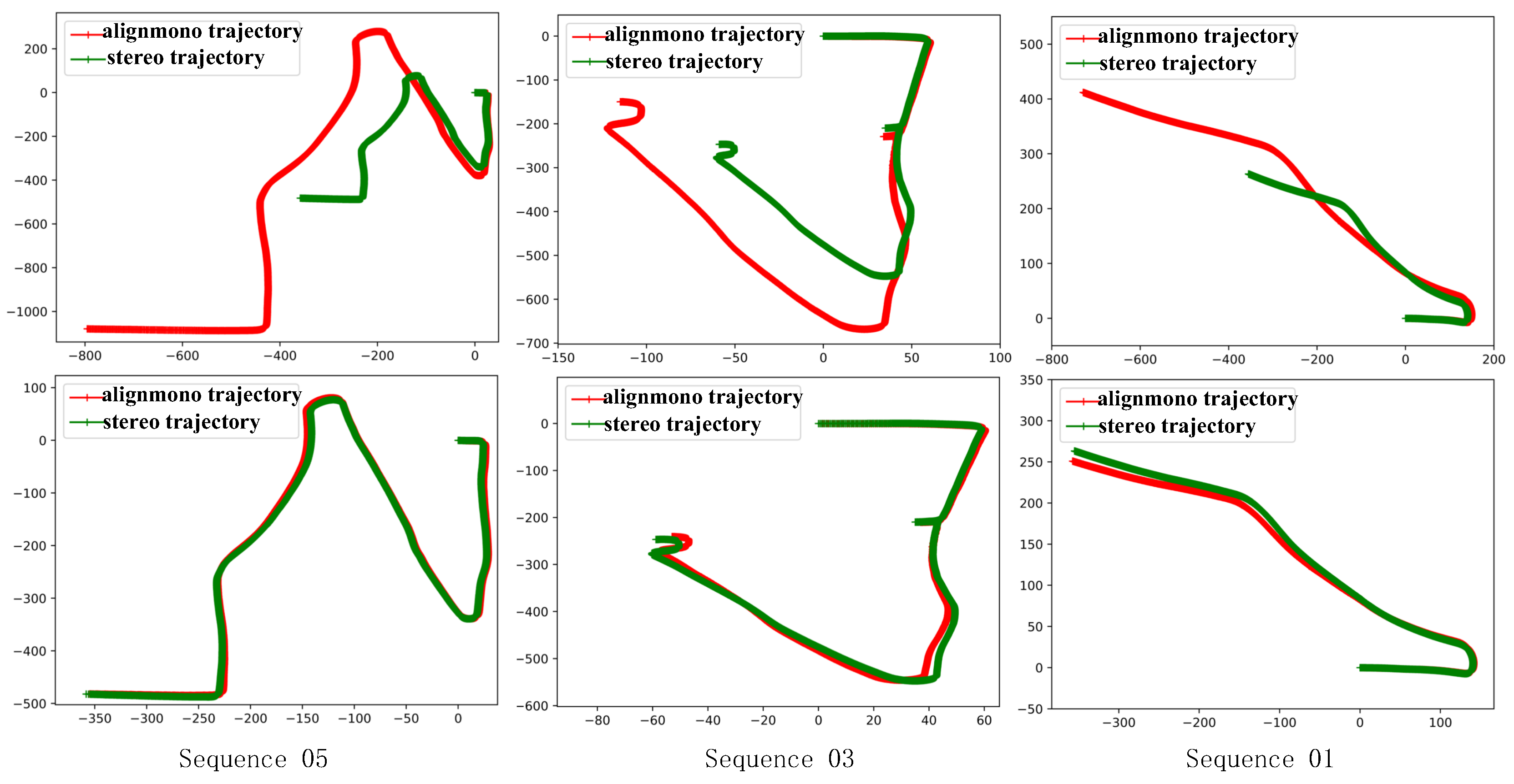
3.2. Evaluation of Scale Estimation Method
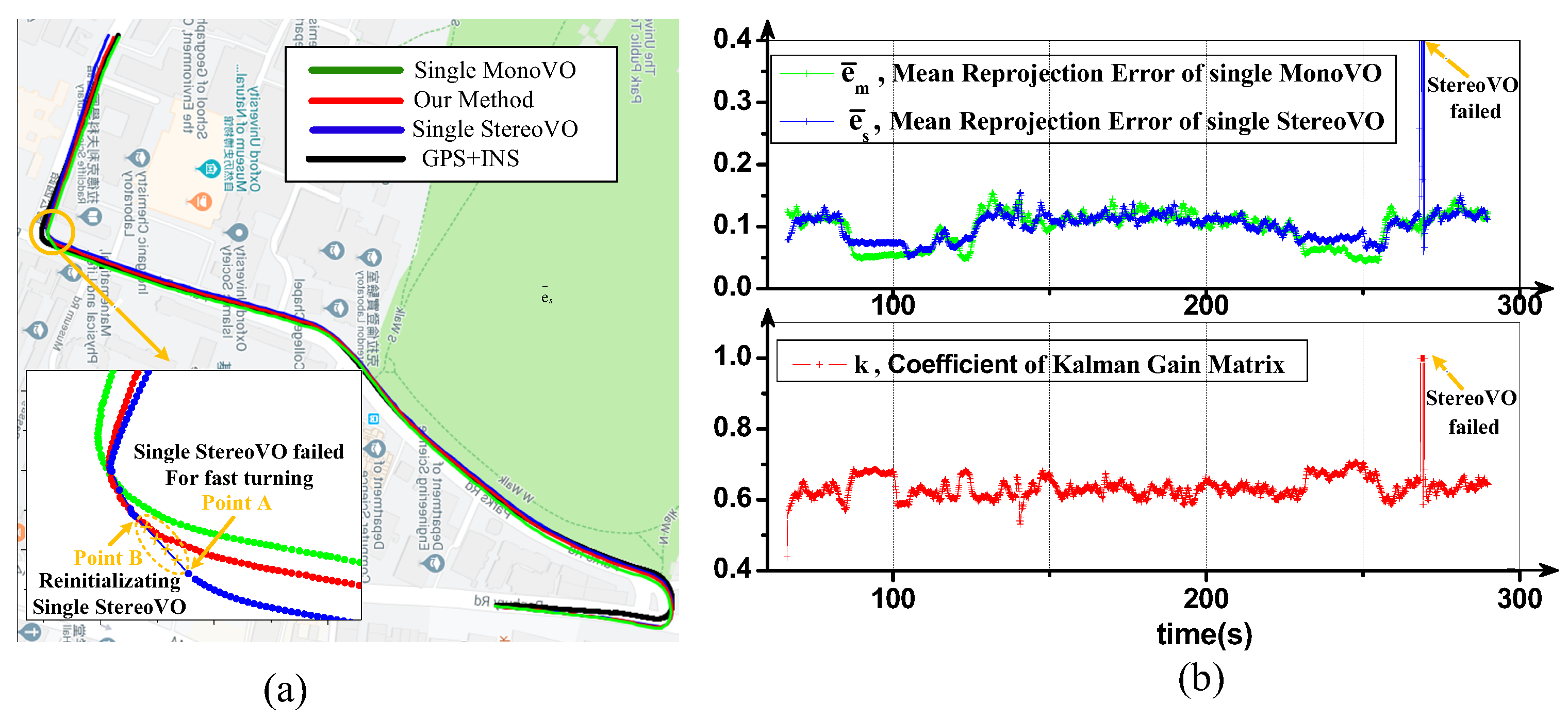
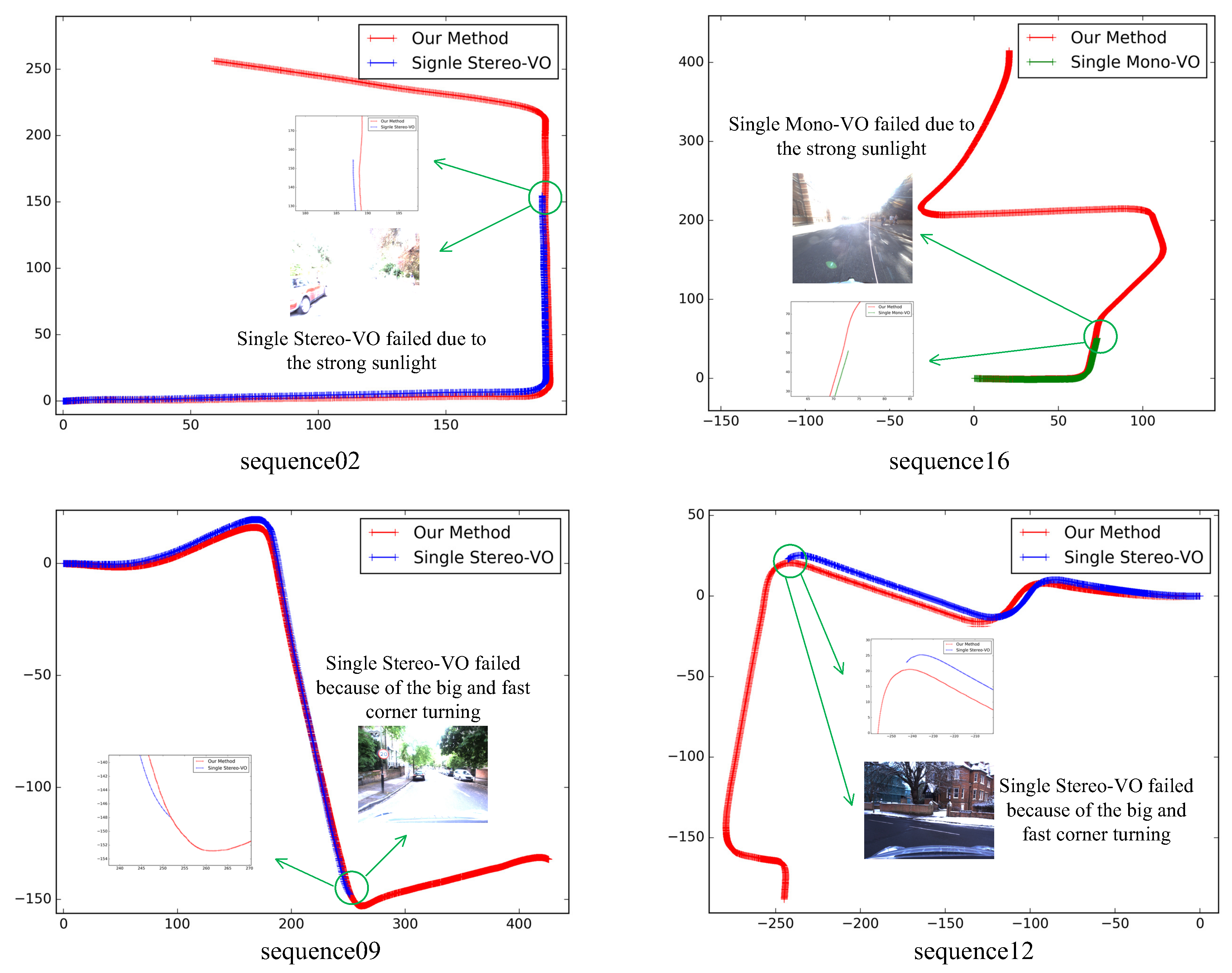
3.3. Robustness Evaluation
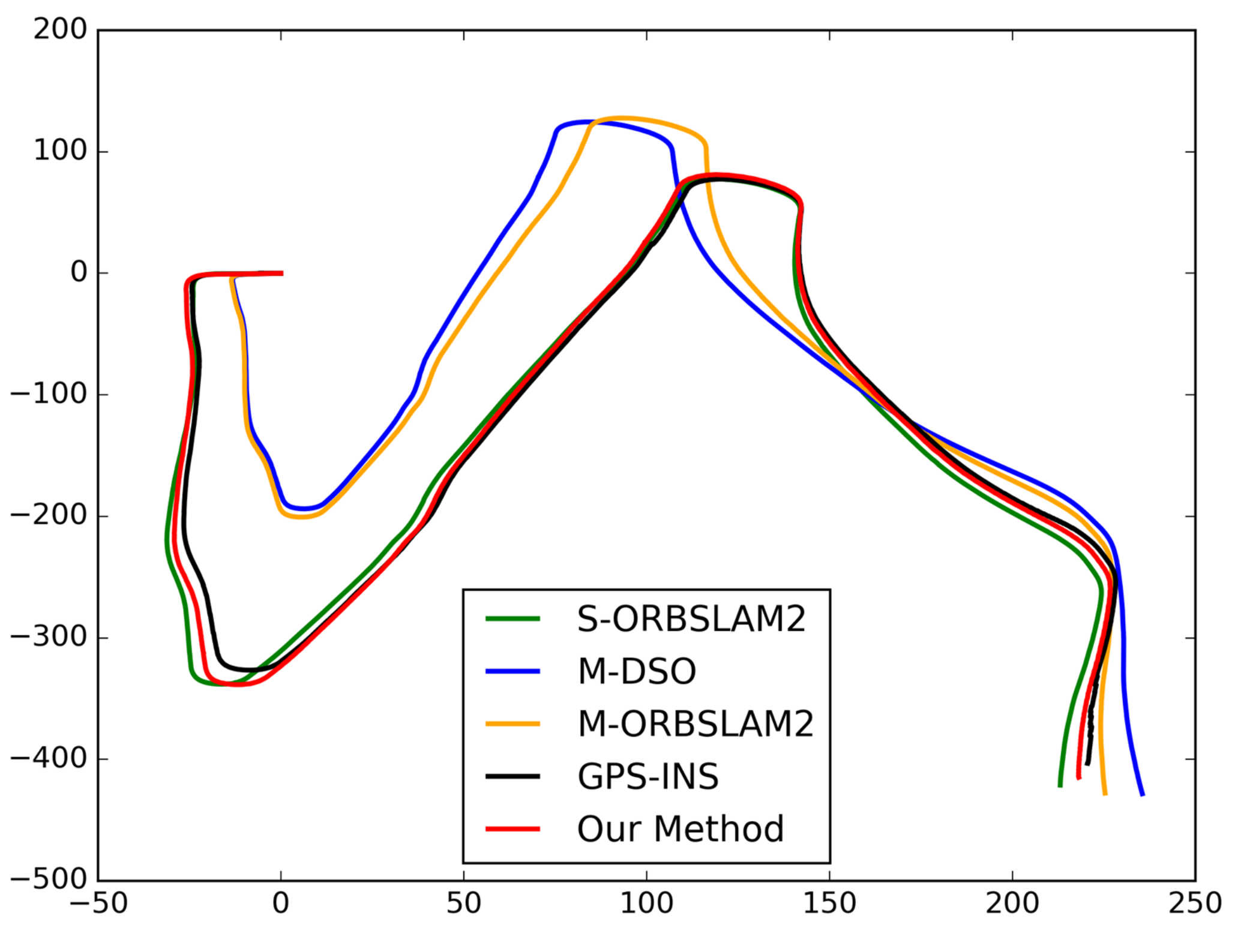
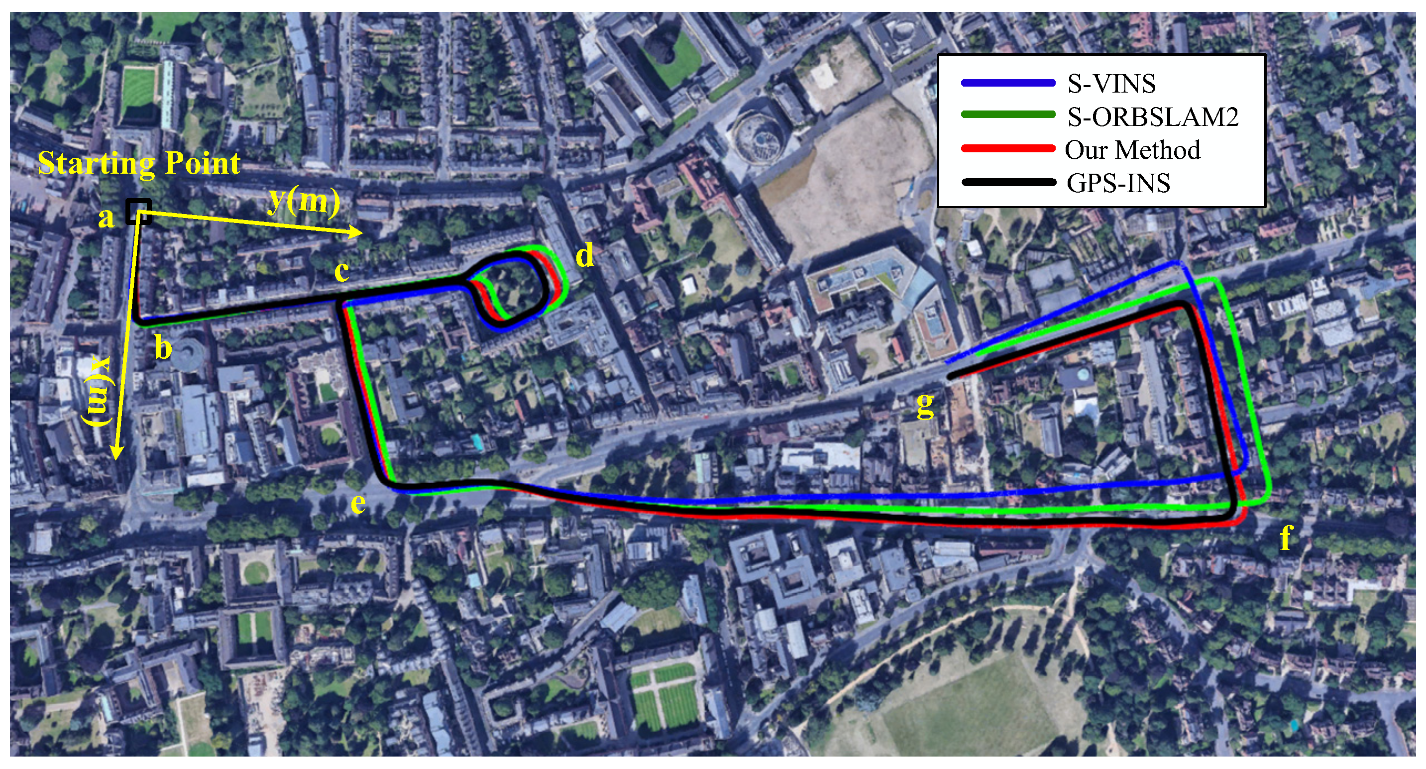
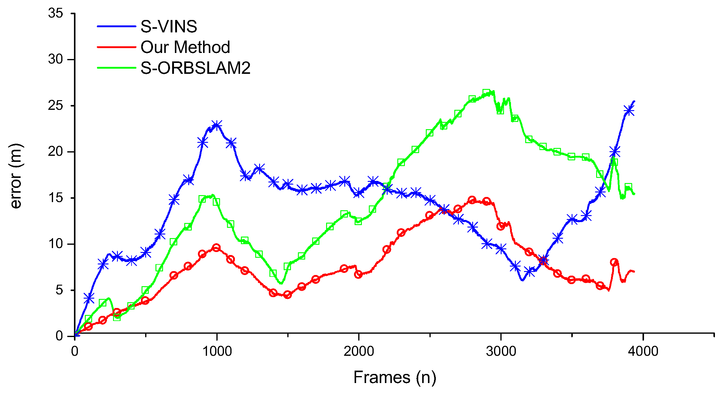
3.4. Accuracy Evaluation
3.5. Time Results
4. Discussion
5. Conclusions
Author Contributions
Funding
Acknowledgments
Conflicts of Interest
Abbreviations
| VO | Visual Odometry |
| GPS | Global Positioning System |
| IMU | Inertial Measurement Unit |
| MSE | Mean Square Error |
| NASA | National Aeronautics and Space Administration |
| SFM | Structure from Motion |
| RANSAC | Random Sample Consensus |
| BA | Bundle Adjustment optimization approach |
| LC | Loop Closure Method |
| RMSE | Root Mean Ssqare Error |
| AEX | Average in X Direction |
| AEY | Average in Y Direction |
| AED | Average in Distance |
References
- Gluckman, J.; Nayar, S.K. Ego-Motion and Omnidirectional Cameras. In Proceedings of the International Conference on Computer Vision, Bombay, India, 7 January 1998. [Google Scholar]
- Gabriele, L.; Maria, S.A. Extended Kalman Filter-Based Methods for Pose Estimation Using Visual, Inertial and Magnetic Sensors: Comparative Analysis and Performance Evaluation. Sensors 2013, 13, 1919–1941. [Google Scholar]
- Wang, K.; Xiong, Z.B. Visual Enhancement Method for Intelligent Vehicle’s Safety Based on Brightness Guide Filtering Algorithm Thinking of The High Tribological and Attenuation Effects. J. Balk. Tribol. Assoc. 2016, 22, 2021–2031. [Google Scholar]
- Chen, J.L.; Wang, K.; Bao, H.H.; Chen, T. A Design of Cooperative Overtaking Based on Complex Lane Detection and Collision Risk Estimation. IEEE Access. 2019, 87951–87959. [Google Scholar] [CrossRef]
- Wang, K.; Huang, Z.; Zhong, Z.H. Simultaneous Multi-vehicle Detection and Tracking Framework with Pavement Constraints Based on Machine Learning and Particle Filter Algorithm. Chin. J. Mech. Eng. 2014, 27, 1169–1177. [Google Scholar] [CrossRef]
- Song, G.; Yin, K.; Zhou, Y.; Cheng, X. A Surveillance Robot with Hopping Capabilities for Home Security. IEEE Trans. Consum. Electron. 2010, 55, 2034–2039. [Google Scholar] [CrossRef]
- Ciuonzo, D.; Buonanno, A.; D’Urso, M.; Palmieri, F.A.N. Distributed Classification of Multiple Moving Targets with Binary Wireless Sensor Networks. In Proceedings of the International Conference on Information Fusion, Chicago, IL, USA, 5–8 July 2011. [Google Scholar]
- Kriechbaumer, T.; Blackburn, K.; Breckon, T.P.; Hamilton, O.; Rivas, C.M. Quantitative Evaluation of Stereo Visual Odometry for Autonomous Vessel Localisation in Inland Waterway Sensing Applications. Sensors 2015, 15, 31869–31887. [Google Scholar] [CrossRef] [PubMed]
- Zhu, J.S.; Li, Q.; Cao, R.; Sun, K.; Liu, T.; Garibaldi, J.M.; Li, Q.Q.; Liu, B.Z.; Qiu, G.P. Indoor Topological Localization Using a Visual Landmark Sequence. Remote Sens. 2019, 11, 73. [Google Scholar] [CrossRef]
- Perez-Grau, F.J.; Ragel, R.; Caballero, F.; Viguria, A.; Ollero, A. An architecture for robust UAV navigation in GPS-denied areas. J. Field Robot. 2018, 35, 121–145. [Google Scholar] [CrossRef]
- Yang, G.C.; Chen, Z.J.; Li, Y.; Su, Z.D. Rapid Relocation Method for Mobile Robot Based on Improved ORB-SLAM2 Algorithm. Remote Sens. 2019, 11, 149. [Google Scholar] [CrossRef]
- Li, Y.; Ruichek, Y. Occupancy Grid Mapping in Urban Environments from a Moving On-Board Stereo-Vision System. Sensors 2014, 14, 10454–10478. [Google Scholar] [CrossRef]
- Scaramuzza, D.; Fraundorfer, F. Visual Odometry [Tutorial]. Robot. Autom. Mag. IEEE 2011, 18, 80–92. [Google Scholar] [CrossRef]
- Chen, J.L.; Wang, K.; Xiong, Z.B. Collision probability prediction algorithm for cooperative overtaking based on TTC and conflict probability estimation method. Int. J. Veh. Des. 2018, 77, 195–210. [Google Scholar] [CrossRef]
- Yang, N.; Wang, R.; Gao, X.; Cremers, D. Challenges in Monocular Visual Odometry: Photometric Calibration, Motion Bias and Rolling Shutter Effect. IEEE Robot. Autom. Lett. 2017, 3, 2878–2885. [Google Scholar] [CrossRef]
- Mou, X.Z.; Wang, H. Wide-Baseline Stereo-Based Obstacle Mapping for Unmanned Surface Vehicles. Sensors 2018, 18, 1085. [Google Scholar] [CrossRef] [PubMed]
- Scaramuzza, D. 1-Point-RANSAC Structure from Motion for Vehicle-Mounted Cameras by Exploiting Non-holonomic Constraints. Int. J. Comput. Vis. 2011, 95, 74–85. [Google Scholar] [CrossRef]
- Zhang, J.; Singh, S. Laser-visual-inertial odometry and mapping with high robustness and low drift. J. Field Robot. 2018, 35, 1242–1264. [Google Scholar] [CrossRef]
- Siddiqui, R.; Khatibi, S. Robust visual odometry estimation of road vehicle from dominant surfaces for large-scale mapping. IET Intell. Transp. Syst. 2014, 9, 314–322. [Google Scholar] [CrossRef]
- Ji, Z.; Singh, S. Visual-Lidar Odometry and Mapping: Low-Drift, Robust, and Fast. In Proceedings of the IEEE International Conference on Robotics and Automation, Seattle, WA, USA, 26–30 May 2015. [Google Scholar]
- Demaeztu, L.; Elordi, U.; Nieto, M.; Barandiaran, J.; Otaegui, O. A temporally consistent grid-based visual odometry framework for multi-core architectures. J. Real Time Image Process. 2015, 10, 759–769. [Google Scholar] [CrossRef]
- Longuet-Higgins, H.C. A computer algorithm for reconstructing a scene from two projections. Nature 1981, 293, 133–135. [Google Scholar] [CrossRef]
- Harris, C.G.; Pike, J.M. 3D positional integration from image sequences. Image Vis. Comput. 1988, 6, 87–90. [Google Scholar] [CrossRef]
- Maimone, M.W.; Cheng, Y.; Matthies, L. Two years of Visual Odometry on the Mars Exploration Rovers. J. Field Robot. 2010, 24, 169–186. [Google Scholar] [CrossRef]
- Lategahn, H.; Stiller, C. Vision-Only Localization. IEEE Trans. Intell. Transp. Syst. 2014, 15, 1246–1257. [Google Scholar] [CrossRef]
- Hasberg, C.; Hensel, S.; Stiller, C. Simultaneous Localization and Mapping for Path-Constrained Motion. IEEE Trans. Intell. Transp. Syst. 2012, 13, 541–552. [Google Scholar] [CrossRef]
- Fraundorfer, F.; Scaramuzza, D. Visual Odometry: Part II: Matching, Robustness, Optimization, and Applications. IEEE Robot. Autom. Mag. 2012, 19, 78–90. [Google Scholar] [CrossRef]
- Nistér, D.; Naroditsky, O.; Bergen, J.R. Visual odometry for ground vehicle applications. J. Field Robot. 2010, 23, 3–20. [Google Scholar] [CrossRef]
- Scaramuzza, D.; Fraundorfer, F.; Siegwart, R. Real-Time Monocular Visual Odometry for on-Road Vehicles with 1-Point RANSAC. In Proceedings of the IEEE International Conference on Robotics and Automation, Kobe, Japan, 12–17 May 2009. [Google Scholar]
- Forster, C.; Carlone, L.; Dellaert, F.; Scaramuzza, D. On-Manifold Preintegration for Real-Time Visual-Inertial Odometry. IEEE Trans. Robot. 2017, 33, 1–21. [Google Scholar] [CrossRef]
- Pascoe, G.; Maddern, W.; Tanner, M.; Piniés, P.; Newman, P. Nid-Slam: Robust Monocular Slam Using Normalised Information Distance. In Proceedings of the IEEE Conference on Computer Vision and Pattern Recognition, Honolulu, HI, USA, 21–26 July 2017; pp. 1435–1444. [Google Scholar]
- Nister, D.; Naroditsky, O.; Bergen, J. Visual Odometry. In Proceedings of the IEEE Computer Society Conference on Computer Vision and Pattern Recognition, Washington, DC, USA, 27 June–2 July 2004. [Google Scholar]
- Mur-Artal, R.; Tardos, J.D. ORB-SLAM2: An Open-Source SLAM System for Monocular, Stereo, and RGB-D Cameras. IEEE Trans. Robot. 2017, 33, 1255–1262. [Google Scholar] [CrossRef]
- Taylor, C.J.; Kriegman, D.J. Structure and motion from line segments in multiple images. Pattern Anal. Mach. Intell. IEEE Trans. 1995, 17, 1021–1032. [Google Scholar] [CrossRef]
- Wong, K.Y.K.; Mendonça, P.R.S.; Cipolla, R. Structure and motion estimation from apparent contours under circular motion. Image Vis. Comput. 2002, 20, 441–448. [Google Scholar] [CrossRef]
- Pradeep, V.; Lim, J. Egomotion Using Assorted Features. In Proceedings of the IEEE Computer Society Conference on Computer Vision and Pattern Recognition, San Francisco, CA, USA, 13–18 June 2010. [Google Scholar]
- David, N. An efficient solution to the five-point relative pose problem. IEEE Trans. Pattern Anal. Mach. Intell. 2004, 26, 756–770. [Google Scholar]
- Haralick, B.M.; Lee, C.N.; Ottenberg, K.; Nölle, M. Review and analysis of solutions of the three point perspective pose estimation problem. Int. J. Comput. Vis. 1994, 13, 331–356. [Google Scholar] [CrossRef]
- Song, Y.; Nuske, S.; Scherer, S. A Multi-Sensor Fusion MAV State Estimation from Long-Range Stereo, IMU, GPS and Barometric Sensors. Sensors 2017, 17, 11. [Google Scholar] [CrossRef] [PubMed]
- Khan, N.H.; Adnan, A. Ego-motion estimation concepts, algorithms and challenges: An overview. Multimed. Tools Appl. 2017, 76, 16581–16603. [Google Scholar] [CrossRef]
- Liu, Y.; Chen, Z.; Zheng, W.J.; Wang, H.; Liu, J.G. Monocular Visual-Inertial SLAM: Continuous Preintegration and Reliable Initialization. Sensors 2017, 17, 2613. [Google Scholar] [CrossRef] [PubMed]
- Zhang, Z. A flexible new technique for camera calibration. IEEE Trans. Pattern Anal. Mach. Intel. 2002, 22, 1330–1334. [Google Scholar] [CrossRef]
- Maddern, W.; Pascoe, G.; Linegar, C.; Newman, P. 1 year, 1000 km: The Oxford RobotCar dataset. Int. J. Robot. Res. 2017, 36, 3–15. [Google Scholar] [CrossRef]
- Engel, J.; Koltun, V.; Cremers, D. Direct Sparse Odometry. IEEE Trans. Pattern Anal. Mach. Intell. 2018, 40, 611–625. [Google Scholar] [CrossRef]
- Sturm, J.; Engelhard, N.; Endres, F.; Burgard, W.; Cremers, D. A Benchmark for the Evaluation of RGB-D SLAM Systems. In Proceedings of the IEEE/RSJ International Conference on Intelligent Robots and Systems, Vilamoura, Portugal, 7–12 October 2012. [Google Scholar]
- Qin, T.; Pan, J.; Cao, S.; Shen, S. A General Optimization-based Framework for Local Odometry Estimation with Multiple Sensors. arXiv 2019, arXiv:1901.03638v1. [Google Scholar]
- Yong, L.; Rong, X.; Yue, W.; Hong, H.; Xie, X.; Liu, X.; Zhang, G. Stereo Visual-Inertial Odometry with Multiple Kalman Filters Ensemble. IEEE Trans. Ind. Electron. 2016, 63, 6205–6216. [Google Scholar]


| Steps | Discription | Formula |
|---|---|---|
| 1 | calculate the current predicted value according to the prediction equation | |
| 2 | update the covariance matrix of prediction equation | |
| 3 | calculating kalman gain | |
| 4 | update the predicted value | |
| 5 | update the covariance of the prediction equation |
| Sequence Description | Duaring Time (s) | Frame Numeber | DSO Mono | DSO Stereo | ORBSLAM2 Stereo | OurMethod Fusion | |
|---|---|---|---|---|---|---|---|
| Seq01 | sun, traffic light | 224 | 2485 | T | F | F | T |
| Seq02 | strong sunlight | 206 | 2267 | F | F | F | T |
| Seq03 | ovrecast, sun | 190 | 2096 | T | T | T | T |
| Seq04 | rain, overcast | 109 | 1205 | T | F | T | T |
| Seq05 | overcast, traffic light | 365 | 4027 | T | F | F | T |
| Seq06 | rain, overcast | 151 | 1665 | F | F | T | T |
| Seq07 | dusk, rain | 183 | 2020 | T | F | T | T |
| Seq08 | overcast, loop road | 224 | 2474 | T | T | F | T |
| Seq09 | sun, clouds | 90 | 2690 | F | F | F | T |
| Seq10 | night, dark | 163 | 1795 | T | F | T | T |
| Seq11 | snow | 119 | 1314 | T | T | T | T |
| Seq12 | snow, traffic light | 252 | 2780 | T | T | F | T |
| Seq13 | illumination change | 152 | 1672 | T | T | T | T |
| Seq14 | strong sunlight | 188 | 2112 | T | F | F | T |
| Total | – | – | – | 11/14 | 5/14 | 7/14 | 14/14 |
| Method | Setting | RMSE (m) | RMSE (%) |
|---|---|---|---|
| S-ORBSLAM2 | Stereo | 6.81 | 0.519 |
| M-DSO | Monocular | 44.22 | 3.372 |
| M-ORBSLAM2 | Monocular | 41.90 | 3.195 |
| Our fusion Method | Multicamera | 5.49 | 0.419 |
| Method | AEX (m) | AEY (m) | AED (m) |
|---|---|---|---|
| S-ORBSLAM2 | 5.84 | 12.41 | 14.30 |
| S-VINS | 4.55 | 12.19 | 13.89 |
| Our Method | 1.83 | 7.14 | 7.60 |
| Part | Module | Times (ms) |
|---|---|---|
| Monocular | Feature Extraction | 20.42 ± 4.03 |
| Pose Tracking | 1.54 ± 0.41 | |
| Local Map Tracking | 6.02 ± 1.27 | |
| Keyframe Selecting | 1.12 ± 0.94 | |
| Total | 29.10 ± 6.65 | |
| Stereo | Feature Extraction | 24.19 ± 3.52 |
| Stereo Matching | 15.73 ± 2.44 | |
| Pose Tracking | 2.01 ± 0.34 | |
| Local Map Tracking | 8.81 ± 3.12 | |
| Keyframe Selecting | 2.72 ± 2.68 | |
| Total | 53.46 ± 12.10 | |
| Fusion | Scale Computation | 0.31 ± 0.12 |
| KF fusion | 0.41 ± 0.17 | |
| Total | 0.72 ± 0.29 |
© 2019 by the authors. Licensee MDPI, Basel, Switzerland. This article is an open access article distributed under the terms and conditions of the Creative Commons Attribution (CC BY) license (http://creativecommons.org/licenses/by/4.0/).
Share and Cite
Wang, K.; Huang, X.; Chen, J.; Cao, C.; Xiong, Z.; Chen, L. Forward and Backward Visual Fusion Approach to Motion Estimation with High Robustness and Low Cost. Remote Sens. 2019, 11, 2139. https://doi.org/10.3390/rs11182139
Wang K, Huang X, Chen J, Cao C, Xiong Z, Chen L. Forward and Backward Visual Fusion Approach to Motion Estimation with High Robustness and Low Cost. Remote Sensing. 2019; 11(18):2139. https://doi.org/10.3390/rs11182139
Chicago/Turabian StyleWang, Ke, Xin Huang, JunLan Chen, Chuan Cao, Zhoubing Xiong, and Long Chen. 2019. "Forward and Backward Visual Fusion Approach to Motion Estimation with High Robustness and Low Cost" Remote Sensing 11, no. 18: 2139. https://doi.org/10.3390/rs11182139
APA StyleWang, K., Huang, X., Chen, J., Cao, C., Xiong, Z., & Chen, L. (2019). Forward and Backward Visual Fusion Approach to Motion Estimation with High Robustness and Low Cost. Remote Sensing, 11(18), 2139. https://doi.org/10.3390/rs11182139