Brightness Temperature Sensitivity to Whitecap Fraction at Millimeter Wavelengths


Abstract

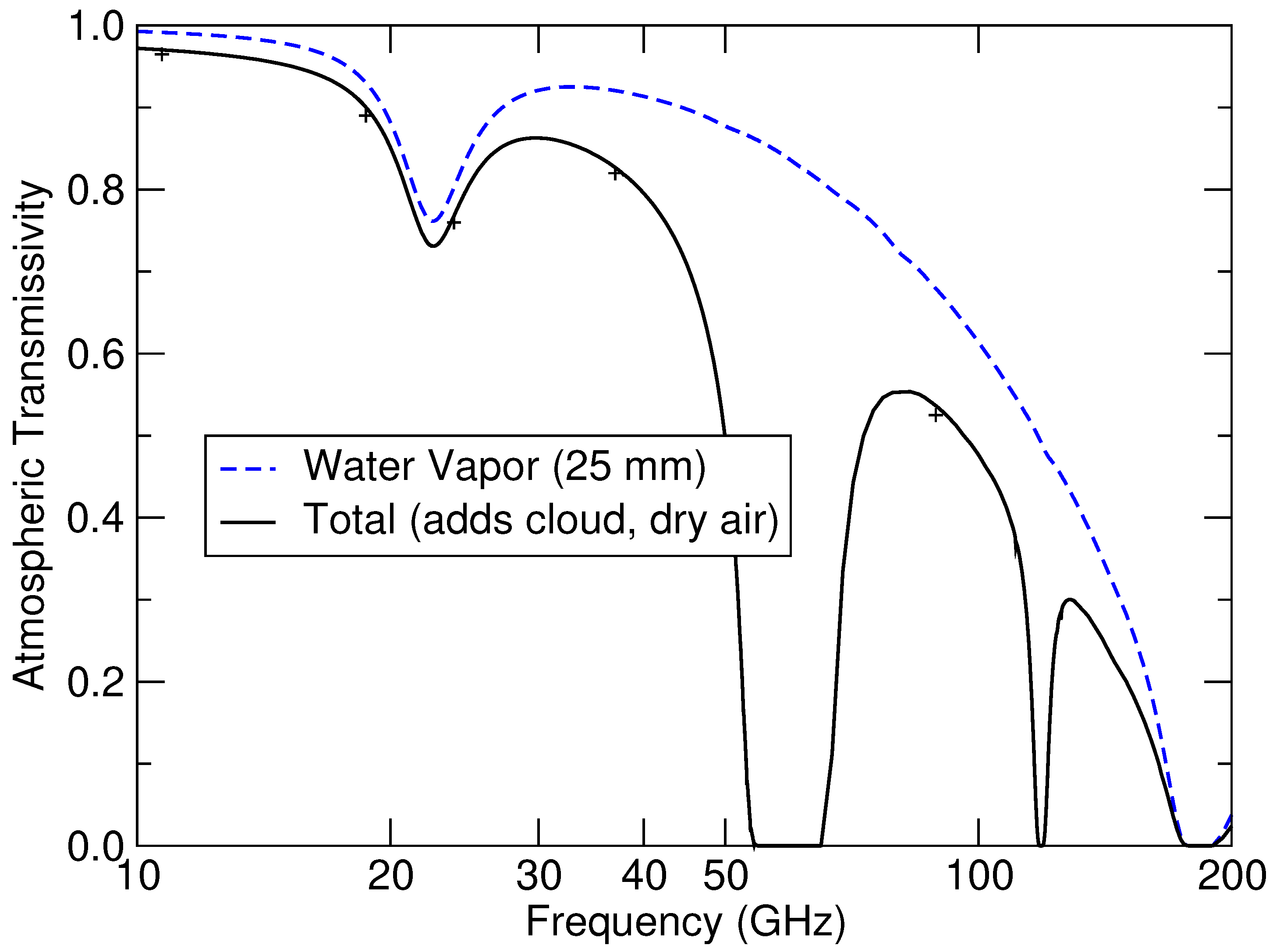
1. Introduction
2. Methods
2.1. Whitecap Fraction Sensitivity Model
2.2. Radiative Transfer Models
2.3. Data
3. Results
4. Discussion
Author Contributions
Funding
Conflicts of Interest
References
- Berry, D.I.; Kent, E.C. A New Air–Sea Interaction Gridded Dataset from ICOADS With Uncertainty Estimates. Bull. Am. Meteorol. Soc. 2009, 90, 645–656. [Google Scholar] [CrossRef]
- Huber, M.B.; Zanna, L. Drivers of uncertainty in simulated ocean circulation and heat uptake. Geophys. Res. Lett. 2017, 44, 1402–1413. [Google Scholar] [CrossRef]
- Fairall, C.W.; Bradley, E.F.; Hare, J.E.; Grachev, A.A.; Edson, J.B. Bulk Parameterization of Air–Sea Fluxes: Updates and Verification for the COARE Algorithm. J. Clim. 2003, 16, 571–591. [Google Scholar] [CrossRef]
- Thorpe, S.A. Bubble clouds and the dynamics of the upper ocean. Q. J. R. Meteorol. Soc. 1992, 118, 1–22. [Google Scholar] [CrossRef]
- Andreas, E.L.; Mahrt, L.; Vickers, D. An improved bulk air–sea surface flux algorithm, including spray-mediated transfer. Q. J. R. Meteorol. Soc. 2015, 141, 642–654. [Google Scholar] [CrossRef]
- Wanninkhof, R.; Asher, W.E.; Ho, D.T.; Sweeney, C.; McGillis, W.R. Advances in Quantifying Air-Sea Gas Exchange and Environmental Forcing. Ann. Rev. Mar. Sci. 2009, 1, 213–244. [Google Scholar] [CrossRef] [PubMed]
- De Leeuw, G.; Andreas, E.L.; Anguelova, M.D.; Fairall, C.W.; Lewis, E.R.; O’Dowd, C.; Schulz, M.; Schwartz, S.E. Production flux of sea spray aerosol. Rev. Geophys. 2011, 49. [Google Scholar] [CrossRef]
- Monahan, E.C. Oceanic Whitecaps. J. Phys. Oceanogr. 1971, 1, 139–144. [Google Scholar] [CrossRef]
- Callaghan, A.H.; White, M. Automated Processing of Sea Surface Images for the Determination of Whitecap Coverage. J. Atmos. Ocean. Technol. 2009, 26, 383–394. [Google Scholar] [CrossRef]
- Brumer, S.E.; Zappa, C.J.; Brooks, I.M.; Tamura, H.; Brown, S.M.; Blomquist, B.W.; Fairall, C.W.; Cifuentes-Lorenzen, A. Whitecap Coverage Dependence on Wind and Wave Statistics as Observed during SO GasEx and HiWinGS. J. Phys. Oceanogr. 2017, 47, 2211–2235. [Google Scholar] [CrossRef]
- Anguelova, M.D.; Bettenhausen, M.H. Whitecap Fraction From Satellite Measurements: Algorithm Description. J. Geophys. Res. Oceans 2019, 124, 1827–1857. [Google Scholar] [CrossRef]
- Salisbury, D.J.; Anguelova, M.D.; Brooks, I.M. On the variability of whitecap fraction using satellite-based observations. J. Geophys. Res. Oceans 2013, 118, 6201–6222. [Google Scholar] [CrossRef]
- Salisbury, D.J.; Anguelova, M.D.; Brooks, I.M. Global distribution and seasonal dependence of satellite-based whitecap fraction. Geophys. Res. Lett. 2014, 41, 1616–1623. [Google Scholar] [CrossRef]
- Albert, M.F.; Anguelova, M.D.; Manders, A.M.; Schaap, M.; De Leeuw, G. Parameterization of oceanic whitecap fraction based on satellite observations. Atmos. Chem. Phys. 2016, 16, 13725–13751. [Google Scholar] [CrossRef]
- Bettenhausen, M.H.; Smith, C.K.; Bevilacqua, R.M.; Wang, N.Y.; Gaiser, P.W.; Cox, S. A Nonlinear Optimization Algorithm for WindSat Wind Vector Retrievals. IEEE Trans. Geosci. Remote Sens. 2006, 44, 597–610. [Google Scholar] [CrossRef]
- Gaiser, P.W.; St. Germain, K.M.; Twarog, E.M.; Poe, G.A.; Purdy, W.; Richardson, D.; Grossman, W.; Jones, W.L.; Spencer, D.; Golba, G.; et al. The WindSat Spaceborne Polarimetric Microwave Radiometer: Sensor Description and Early Orbit Performance. IEEE Trans. Geosci. Remote Sens. 2004, 42, 2347–2361. [Google Scholar] [CrossRef]
- Greenert, J.W. The United States Navy Arctic Roadmap for 2014 to 2030; Office of the Chief of Naval Operations: Washington DC, USA, 2014. [Google Scholar]
- Ulaby, F.; Moore, R.; Fung, A. Microwave Remote Sensing: Active and Passive, Volume 1: Microwave Remote Sensing: Fundamentals and Radiometry; Addison-Wesley: Reading, MA, USA, 1981; pp. 344–427. [Google Scholar]
- Potter, H.; Smith, G.B.; Snow, C.M.; Dowgiallo, D.J.; Bobak, J.P.; Anguelova, M.D. Whitecap lifetime stages from infrared imagery with implications for microwave radiometric measurements of whitecap fraction. J. Geophys. Res. Oceans 2015, 120, 7521–7537. [Google Scholar] [CrossRef]
- Iturbide-Sanchez, F.; Reising, S.C.; Padmanabhan, S. A Miniaturized Spectrometer Radiometer Based on MMIC Technology for Tropospheric Water Vapor Profiling. IEEE Trans. Geosci. Remote Sens. 2007, 45, 2181–2194. [Google Scholar] [CrossRef]
- Osaretin, I.A.; Shields, M.W.; Lorenzo, J.A.M.; Blackwell, W.J. A Compact 118-GHz Radiometer Antenna for the Micro-Sized Microwave Atmospheric Satellite. IEEE Antennas Wirel. Propag. Lett. 2014, 13, 1533–1536. [Google Scholar] [CrossRef]
- Colomina, I.; Molina, P. Unmanned aerial systems for photogrammetry and remote sensing: A review. ISPRS J. Photogramm. Remote Sens. 2014, 92, 79–97. [Google Scholar] [CrossRef]
- Rosenkranz, P.W. Rough-sea microwave emissivities measured with the SSM/I. IEEE Trans. Geosci. Remote Sens. 1992, 30, 1081–1085. [Google Scholar] [CrossRef]
- Saunders, R.; Hocking, J.; Turner, E.; Rayer, P.; Rundle, D.; Brunel, P.; Vidot, J.; Roquet, P.; Matricardi, M.; Geer, A.; et al. An update on the RTTOV fast radiative transfer model (currently at version 12). Geosci. Model Dev. 2018, 11, 2717–2737. [Google Scholar] [CrossRef]
- Payne, V.H.; Mlawer, E.J.; Cady-Pereira, K.E.; Moncet, J.L. Water Vapor Continuum Absorption in the Microwave. IEEE Trans. Geosci. Remote Sens. 2011, 49, 2194–2208. [Google Scholar] [CrossRef]
- English, S.J.; Hewison, T.J. Fast generic millimeter-wave emissivity model. Proc. SPIE 1998, 3503, 288. [Google Scholar] [CrossRef]
- Deblonde, D.; English, S.J. Evaluation of the FASTEM2 fast microwave oceanic surface emissivity model. In Technical Proceedings of the Eleventh International ATOVS Study Conference; Le Marshall, J.F., Jasper, J.D., Eds.; Australia Bureau of Meteorology: Budapest, Hungary, 2000; pp. 67–78. [Google Scholar]
- Liu, Q.; Weng, F.; English, S.J. An Improved Fast Microwave Water Emissivity Model. IEEE Trans. Geosci. Remote Sens. 2011, 49, 1238–1250. [Google Scholar] [CrossRef]
- Bormann, N.; Geer, A.; English, S.J. Evaluation of The Microwave Ocean Surface Emissivity Model FASTEM-5 in the IFS; Technical Report Technical Memorandum 667; ECMWF: Reading, UK, 2012. [Google Scholar]
- Kazumori, M.; Shibata, A.; English, S.J. Asymmetric Features of Oceanic Microwave Brightness Temperature in HighSurface Wind Speed Condition. IEEE Trans. Geosci. Remote Sens. 2015, 53, 5901–5914. [Google Scholar] [CrossRef]
- Durden, S.L.; Vesecky, J.F. A Physical Radar Cross-Section Model for a Wind-Driven Sea with Swell. IEEE J. Ocean. Eng. 1985, 10, 445–451. [Google Scholar] [CrossRef]
- Stogryn, A. The emissivity of sea foam at microwave frequencies. J. Geophys. Res. (1896–1977) 1972, 77, 1658–1666. [Google Scholar] [CrossRef]
- Rose, L.A.; Asher, W.E.; Reising, S.C.; Gaiser, P.W.; Germain, K.M.S.; Dowgiallo, D.J.; Horgan, K.A.; Farquharson, G.; Knapp, E.J. Radiometric Measurements of the Microwave Emissivity of Foam. IEEE Trans. Geosci. Remote Sens. 2002, 40, 2619–2625. [Google Scholar] [CrossRef]
- European Centre for Medium-Range Weather Forecasts. ERA-Interim Project; Research Data Archive at the National Center for Atmospheric Research, Computational and Information Systems Laboratory: Boulder, CO, USA, 2018. [Google Scholar]
- Zweng, M.; Reagan, J.; Antonov, J.; Locarnini, R.; Mishonov, A.; Boyer, T.; Garcia, H.; Baranova, O.; Johnson, D.; Seidov, D.; et al. World Ocean Atlas 2013, Volume 2: Salinity; Technical Report 74; NOAA Atlas NESDIS: Silver Spring, MD, USA, 2013. [Google Scholar]
- Hollinger, J.P. Passive Microwave Measurements of Sea Surface Roughness. IEEE Trans. Geosci. Electron. 1971, 9, 165–169. [Google Scholar] [CrossRef]
- Anguelova, M.D.; Gaiser, P.W. Skin depth at microwave frequencies of sea foam layers with vertical profile of void fraction. J. Geophys. Res. Oceans 2011, 116. [Google Scholar] [CrossRef]
- Anguelova, M.D.; Gaiser, P.W. Dielectric and Radiative Properties of Sea Foam at Microwave Frequencies: Conceptual Understanding of Foam Emissivity. Remote Sens. 2012, 4, 1162–1189. [Google Scholar] [CrossRef]


| Frequency (GHz) | 53 EIA | 0 (nadir) | ||||||
|---|---|---|---|---|---|---|---|---|
| Altitude (km) | Altitude (km) | |||||||
| TOA | 1 | 0.5 | Surface | TOA | 1 | 0.5 | Surface | |
| 37 | 127.3 | 141.9 | 145.8 | 150.4 | 122.1 | 132.4 | 134.9 | 137.8 |
| 89 | 56.2 | 74.0 | 82.0 | 91.8 | 62.6 | 73.4 | 77.6 | 82.5 |
| 113 | 23.0 | 40.1 | 47.6 | 57.9 | 33.7 | 46.9 | 51.9 | 57.8 |
| 150 | 10.9 | 20.7 | 27.5 | 38.4 | 19.4 | 28.5 | 33.8 | 41.4 |
© 2019 by the authors. Licensee MDPI, Basel, Switzerland. This article is an open access article distributed under the terms and conditions of the Creative Commons Attribution (CC BY) license (http://creativecommons.org/licenses/by/4.0/).
Share and Cite
Bettenhausen, M.H.; Anguelova, M.D. Brightness Temperature Sensitivity to Whitecap Fraction at Millimeter Wavelengths. Remote Sens. 2019, 11, 2036. https://doi.org/10.3390/rs11172036
Bettenhausen MH, Anguelova MD. Brightness Temperature Sensitivity to Whitecap Fraction at Millimeter Wavelengths. Remote Sensing. 2019; 11(17):2036. https://doi.org/10.3390/rs11172036
Chicago/Turabian StyleBettenhausen, Michael H., and Magdalena D. Anguelova. 2019. "Brightness Temperature Sensitivity to Whitecap Fraction at Millimeter Wavelengths" Remote Sensing 11, no. 17: 2036. https://doi.org/10.3390/rs11172036
APA StyleBettenhausen, M. H., & Anguelova, M. D. (2019). Brightness Temperature Sensitivity to Whitecap Fraction at Millimeter Wavelengths. Remote Sensing, 11(17), 2036. https://doi.org/10.3390/rs11172036