Article

Improving SWE Estimation by Fusion of Snow Models with Topographic and Remotely Sensed Data

by
Ludovica De Gregorio
1,2,*,
Daniel Günther
3,
Mattia Callegari
1,
Ulrich Strasser
3,
Marc Zebisch
1,
Lorenzo Bruzzone
2 and
Claudia Notarnicola
1
1
Institute for Earth Observation, European Academy of Bozen / Bolzano, EURAC Research, viale Druso, 1-39100 Bolzano, Italy
2
Department of Information Engineering and Computer Science, University of Trento, Via Sommarive, 9, I-38123 Trento, Italy
3
Department of Geography, University of Innsbruck, Innrain 52f, 6020 Innsbruck, Austria
*
Author to whom correspondence should be addressed.
Remote Sens. 2019, 11(17), 2033; https://doi.org/10.3390/rs11172033
Submission received: 8 July 2019 / Revised: 23 August 2019 / Accepted: 27 August 2019 / Published: 29 August 2019

Abstract

:
This paper presents a new concept to derive the snow water equivalent (SWE) based on the joint use of snow model (AMUNDSEN) simulation, ground data, and auxiliary products derived from remote sensing. The main objective is to characterize the spatial-temporal distribution of the model-derived SWE deviation with respect to the real SWE values derived from ground measurements. This deviation is due to the intrinsic uncertainty of any theoretical model, related to the approximations in the analytical formulation. The method, based on the k-NN algorithm, computes the deviation for some labeled samples, i.e., samples for which ground measurements are available, in order to characterize and model the deviations associated to unlabeled samples (no ground measurements available), by assuming that the deviations of samples vary depending on the location within the feature space. Obtained results indicate an improved performance with respect to AMUNDSEN model, by decreasing the RMSE and the MAE with ground data, on average, from 154 to 75 mm and from 99 to 45 mm, respectively. Furthermore, the slope of regression line between estimated SWE and ground reference samples reaches 0.9 from 0.6 of AMUNDSEN simulations, by reducing the data spread and the number of outliers.

Graphical Abstract

1. Introduction

Melt water from snow and glaciers plays a key role in the hydrological cycle by contributing to the river flow and water resources in many parts of the world. It is estimated that about one-sixth of the world’s population depends on snow- and ice-melt for the supply with drinking water [1]. Therefore, for hydrological assessments in these regions, knowledge about the spatial and temporal distribution of the snow water equivalent (SWE) is of uttermost importance.
SWE is defined as the amount of water contained within the snowpack: It can be thought as the depth of water that would theoretically result if the entire snowpack would melt instantaneously [2]. Where available, point ground measurements of SWE remain the main direct information about the snow mass. However, given the large spatial heterogeneity of snow they may not be representative of large areas. A spatialized estimation of SWE in mountain areas, which are typically complex terrains with high topographic heterogeneity, is currently one of the most important challenges of snow hydrology [3]. An improved knowledge of the spatial distribution of SWE and its evolution over time would allow a better management of mountain water resources for drinking water supply, agriculture and hydropower, as well as for flood protection.
In literature, several approaches to the estimation of the spatial distribution of SWE exist. One of the most common methods is the interpolation of SWE ground measurements, constrained by remotely sensed maps of the snow extent. If enough ground measurements with a good spatial distribution are available, this approach may produce accurate SWE results [4]. Two different types of snow extent products derived from satellite exist: fractional and binary snow cover maps. Fassnacht et al. [4] and Molotch et al. [5] use of the fractional product that provides information about the percentage (from 0% to 100%) of snow coverage for each pixel. Elder et al. [6], instead, utilize binary mapping techniques with a set of thresholds to determine whether a pixel is snow-covered or not. A common statistical technique for spatial interpolation is based on binary regression trees that have been successfully applied to obtain interpolated SWE values from ground observations [6,7]. However, numerous studies show that individual point observations of SWE are not necessarily representative of the surrounding area [8,9,10], thus limiting the feasibility of this approach.
Several statistical models have been developed to spatially interpolate the point-based snow information, e.g., multivariate linear regression can relate physiographic variables, historical SWE data and snow-covered area imagery to the observed SWE. The accuracy of this simple method can be better than those of more complex techniques such as inverse-distance weighting [11].
Due to their accuracy and ability to preserve patterns from observations [12], nearest-neighbor approaches are an alternative methodical approach for spatio-temporal modeling biophysical parameters. However, in literature, only few studies exist based on the use of k-NN algorithms for modeling snow parameters. Among them, Zheng et al. [12] developed an approach to estimate SWE through the interpolation of spatially representative point measurements using a k-NN algorithm and historical spatial SWE data. Schneider et al. [13] estimated the relationships between SWE, snow covered area and topography to extend the Airborne Snow Observatory (ASO) dataset. In their analysis, they also used a nearest neighbor approach for resampling fractional snow-covered area maps.
Another common approach for retrieving spatially distributed SWE is the reconstruction based on both remotely sensed snow cover maps and the estimation of snowmelt. The main idea, developed by Martinec and Rango [14], is to identify the date of snow disappearance for each pixel starting from Landsat snow cover maps; then, through a backward calculation of the melt rate, the accumulated SWE for each day back to the last significant snowfall is reconstructed. The sources of uncertainty for this approach are mainly related to the melt model structure and its meteorological forcing. Moreover, the main disadvantage of this approach is that it works properly only in areas with distinct accumulation and ablation periods. Furthermore, it operates retroactively only after snow disappearance, and hence does not enable the application for streamflow forecasting. Bair et al. [15] validated two different SWE reconstruction methods with the NASA ASO data in the upper Tuolumne River Basin in California’s Sierra Nevada. The first approach uses an energy balance model to calculate snowmelt, integrating different remotely sensed products like daily MODIS fractional snow-covered area and albedo; it also considers ephemeral snow (i.e., snow that rapidly appears and disappears). The second reconstruction model implements a net radiation restricted degree-day approach [16]. The first method results, on average, more accurate than the second one in the SWE reconstruction, by showing no bias (0%) and a low mean absolute error (26%). Other successful examples of reconstructed SWE for basins in Sierra Nevada are shown by Girotto et al. [17], Guan et al. [18] and Rittger et al. [19].
An accurate estimation of SWE from remotely sensed images represents a longstanding challenge. Satellite data in the visible bands may provide information about the presence or absence of snow cover [20] but require cloud-free conditions. However, no indication on the total amount of the snow mass can be derived. Passive microwave (PM) instruments are able to estimate the brightness temperature naturally emitted from the Earth and can be used to estimate SWE. When snow covers the ground, microwave radiation transmitted through the snowpack is absorbed and scattered by snow grains by decreasing the measured radiation. A deeper snowpack includes a larger number of snow grains, which are the main responsible for signal attenuation. This inverse relationship between snow depth and temperature brightness is the basis of SWE retrieval from PM measurements [21]. Vuyovich and Jacobs [21] compared snow hydrology model results to remotely sensed data to determine if passive microwave estimates of SWE can be used to characterize the snowpack and estimate runoff from snowmelt in the Helmand River, in Afghanistan. Mizukami and Perica [22] tried to identify SWE retrieval algorithms feasible for large-scale operational applications. In their study, Vuyovich et al. [23] compared the daily AMSR-E and SSM/I SWE products over nine winter seasons with spatially distributed model output of the SNOw Data Assimilation System (SNODAS) at watershed scale (25 km of spatial resolution) for 2100 watersheds in the United States. Results show large areas where the passive microwave SWE products are highly correlated to the SNODAS data, except in heavily forested areas and regions with a deep snowpack, where passive microwave SWE is significantly underestimated with respect to SNODAS. The best correlation is associated with basins in which maximum annual SWE value is lower than 200 mm and forest fraction is less than 20%. Forest cover has been proven to be one of the most relevant sources of uncertainty in SWE retrieval with PM sensors by acting as a mask for the snowpack microwave emission [24,25]. Moreover, snow metamorphism affects the snowpack microwave emission by changing the crystal sizes, caused by temperature and water vapor gradients [26,27]. Finally, SWE estimation from PM sensors suffers from several issues related to the coarse spatial resolution of the sensors (~25 km): In mountain regions, indeed, the spatial variability of snow cover and snow properties over a 25-km grid is large due to topographic influences.
In the last decades, scientists have also extensively investigated the potential of Synthetic Aperture Radar (SAR) data for deriving SWE. Sun et al. [28] used microwave scattering models to analyze the C-band SAR scattering characteristics of snow-covered areas and estimated the distribution of the SWE using SAR data and snow cover data measured in the field. Conde et al. [29] presented a methodology for mapping the temporal variation of SWE through the SAR Interferometry technique and Sentinel-1 data.
Information about snow state variables can also be obtained from hydrological models. Many of the existing snowpack models are based on the same physical principles and solve the surface energy balance problem of a snowpack [30]. The main difference among these models is related to the way they represent physical processes in the snowpack such as absorption of incoming radiation, advection and convection, and how they represent the internal structure of the snowpack. In a cross-comparison with 33 models, Rutter et al. [30] found that the correlation of models’ performance between years is always stronger at the open sites than in the forest, suggesting that models are more robust at open sites.
The increasing complexity of snow-cover models demands high-quality forcing data. However, meteorological forcing data as provided by weather station recordings or atmospheric simulations suffer from several errors such as those induced by inaccuracy of the measurement, the regionalization scheme or boundary conditions. The process representations in deterministic, physically based snow models (which simulate physical processes in the snowpack) are an abstraction of reality, and hence inherently introduce uncertainty through simplification and the choice of parameter values. For fully distributed snow models, the spatial resolution is a compromise between computational feasibility and adequacy in mirroring the spatial scale of physical processes. Especially if the resolution (i.e., cell size) is much larger than the processes considered in the model, this choice is associated with uncertainty.
On the basis of this analysis, the main objective of this work is to generate a spatialized product of SWE over an Alpine area composed of Tyrol, South Tyrol and Trentino (Euregio region), by overcoming the aforementioned problems of hydrological models related to intrinsic uncertainty of the forcing data and correcting the spatial-temporal distribution of SWE as simulated by the snow model AMUNDSEN. The correction is performed using a specific k-NN algorithm and exploiting ground measurement-derived SWE data. The innovative aspect of our work is the joint use of snow model simulations, ground data, auxiliary products based on remote sensing and an advanced estimation technique to derive SWE. In this way our approach differs from traditional data assimilation techniques.
The paper is organized as follows: Section 2 introduces the study area and, after a description of the dataset, the method for SWE retrieval is presented in the last part of the section results are then shown and discussed in Section 3 and, finally, conclusions and future perspectives are drawn in Section 4.

2. Materials and Methods

2.1. Study Area

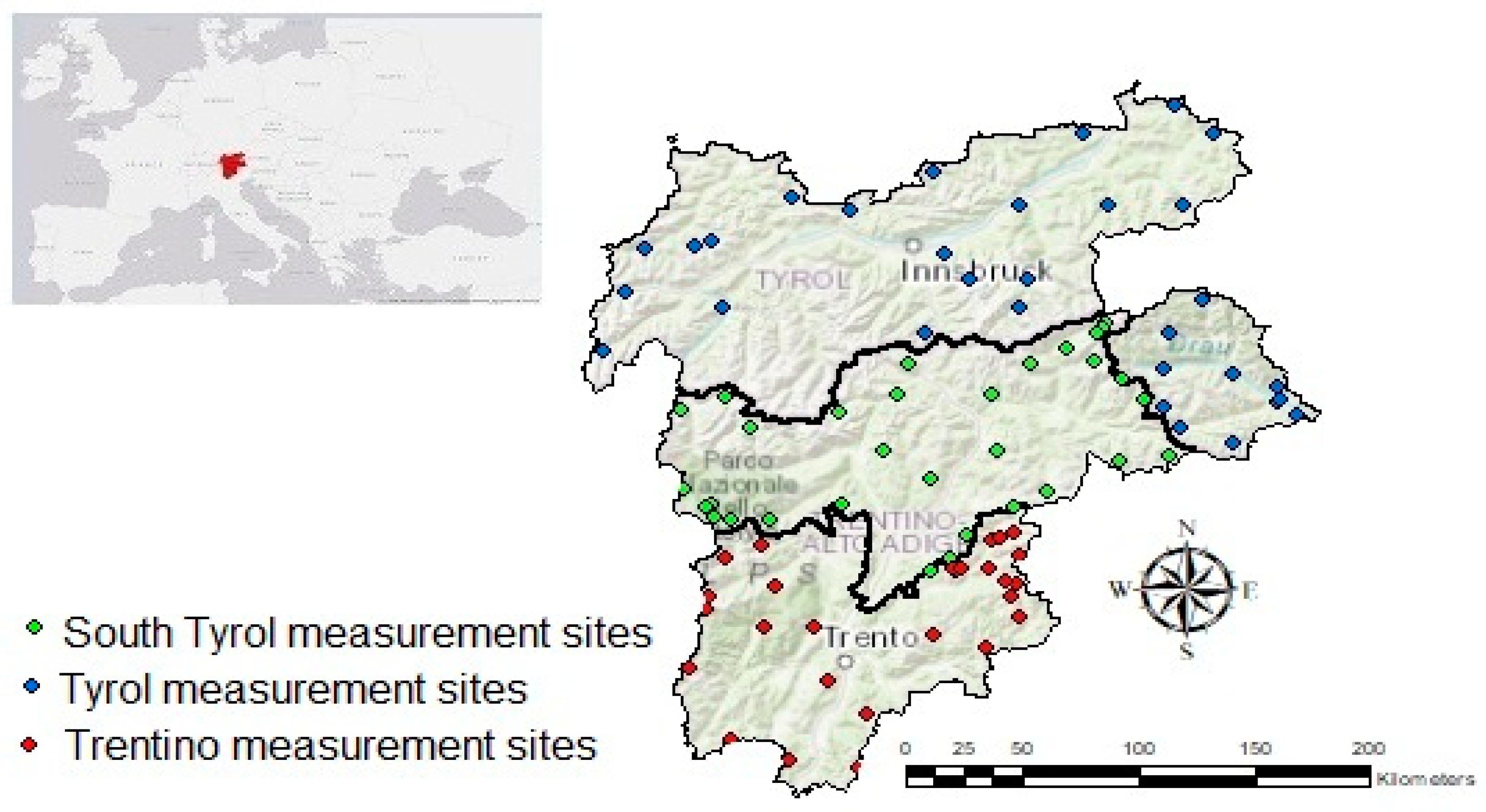
The considered study area is the Alpine region that includes Tyrol (Austria), and South Tyrol and Trentino (North-East Italy, Figure 1). Most of the rivers in the central and northern part of the considered region have a nivo-glacial regime with maximum discharge during the late summer months, whereas in the southern part of Trentino maximum discharge usually occurs during spring with an earlier snowmelt [31]. The area is covered by a relatively dense network of measurements sites (Figure 1), where snow profiles are periodically collected by the operators of the Avalanche Offices of the Provinces of Trento and of Bolzano (for Trentino and South Tyrol, respectively) and by the Hydrographic Service and the Zentralanstalt für Meteorologie und Geodynamik (ZAMG) for the Tyrol region.

2.2. Data Description

This section describes the input (features) and the target variables used in the proposed method. The same features have been selected for the three regions. Table 1 summarizes the features selected for implementing the k-NN algorithm and, below, shows the number of SWE ground samples available for each region. The following subsections will describe the single features used in the analyses.

2.2.1. The AMUNDSEN Model and Its Uncertainty

SWE is simulated using the distributed, physically based snow model AMUNDSEN (“Alpine MUltiscale Numerical Distributed Simulation ENgine”) [32]. The regionalization and approximation of measured and unmeasured meteorological forcing and the inclusion of snow-canopy interactions are performed by the meteorological preprocessor of the model. Then the coupled mass- and energy-balance is solved at every raster cell by means of the energy balance scheme of the integrated 1-D Factorial Snowpack Model (FSM) [33]. AMUNDSEN has proven its performance in a variety of applications in different natural environments [34]. In our application, the model has been validated at 38 stations with automated snow depth recordings. Additionally, 16 stations operated by the Hydrographic Service of the Province of Bolzano provide recordings of the snow surface temperature to validate the mass and energy balance separately. Daily snow height was predicted with a mean Nash-Sutcliffe efficiency (NSE) of 0.68 (ranging from 0.25 to 0.96).
In this work three snowpack variables provided by AMUNDSEN are used as features for implementing the k-NN algorithm: (i) SWE, corresponding to location and date of respective ground measurements, (ii) the associated uncertainty value, and (iii) a “SWE climatology” parameter. The latter is the average of the SWE values at the point and for the date corresponding to the ground measurement calculated for the other years. The uncertainty associated to the AMUNDSEN SWE simulation is based on ensemble simulation comparisons. Such ensemble simulations are a common way for assessing the uncertainty of model output. In many disciplines, such as hydrology, meteorology and cryospheric sciences, ensemble simulations have demonstrated their potential in improving the robustness of forecasts [35] and assimilation schemes [36]. In this study we follow a multi-model approach to generate an ensemble and include as many sources of uncertainty as possible.
However, given the large extension of our study site the resulting computational costs need to be considered. In order to resolve critical snow-related processes such as snow redistribution and absorption of incoming shortwave radiation, hourly simulations are carried out with a spatial resolution of 250 × 250m. A maximum of 96 ensemble members were considered feasible, parallelized on a 96-core cluster. In order to reduce the number of the ensemble members while still enabling a certain amount of dispersion, just the most sensitive model configurations, i.e., those that explain most of the output variance, are accounted for.
An uncertainty and sensitivity analysis of FSM at one station in the study region identified the albedo formulations as well as the liquid water transport scheme inside the snowpack as the origin of the highest explanatory power for the performance variance [37]. Errors in precipitation sums and the approximation of the precipitation phase together with errors in air temperature and the radiative forcing are responsible for most uncertainties from a forcing data perspective. We reproduced the spread of a larger ensemble by a manual selection, result of a point-scale sensitivity analysis aimed at identifying the most important uncertainty sources (input data, model structures and parameters choice) to explain the variance of the model performance. The selection is based on the findings of the Guenther et al. study [37]. However, in order to reduce the number of the ensemble members (in this study limited to 96 for computational reasons) while still representing the uncertainty for spatial distributed simulations, we just perturbed some of the most sensitive model settings. Particularly, we considered the following sources of uncertainty:
  • Precipitation phase: The wet-bulb temperature (Tw), obtained through an iterative solution of the psychometric equation, has shown to improve predictions of snow and rainfall transition [38]. Lower and upper wet-bulb temperature limits, between which mixed snow and rainfall events are possible, are set;
  • Precipitation undercatch and errors in elevation gradient and lateral redistribution: Uncertainties associated with these factors are lumped together and their influence is approximated with two different precipitation correction factors;
  • Longwave irradiance: Incoming longwave radiation is sparsely measured in the study area. Therefore, this input variable is derived from recordings of shortwave irradiance, air temperature (Ta), water-vapor content (ea) and the subsequent computation of atmospheric transmissivity and surface temperatures of surrounding slopes [39]. We utilize two different formulations of the clear-sky emissivity (εcs) estimation for a rough uncertainty estimation of this factor;
  • Snow albedo (αs): In FSM two different albedo evolution representations are implemented. The prognostic option decreases albedo as snow ages over a timescale factor τa (with different values for cold and melting snow, respectively) towards a minimum (αmin), and increases albedo according to the amount of fresh snowfall (Sf) relative to a required snowfall amount to refresh the albedo (Sα) to its maximum (αmax). The second option predicts albedo as a function of surface temperature (Ts) in relation to the melting temperature (Tm). We employ both albedo options with two sets of parameters each for minimum and maximum albedo;
  • Snowpack hydraulics: Liquid water in snow layers is parameterized by a simple bucket model, where the maximum amount of liquid water (Wmax) that a snow layer i can contain is dependent on the porosity (φi), the snow layer depth (hi) and the irreducible liquid water content (Wirr). In the ensemble we apply this scheme with three different values of Wirr. Setting Wirr to 0 corresponds to switching off this option.
The combination of all presented model options and parameter sets results in an ensemble with 96 members.

2.2.2. Topographic and Auxiliary Parameters

This section refers to all those parameters that do not vary in time and that are used as features in the k-NN algorithm for SWE derivation. Topographic parameters can be used as proxies for the meteorological drivers, such as precipitation or wind for sublimation and redistribution or solar radiation (and temperature) for snowmelt. In addition, vegetation, and in particular the presence and density of a canopy, affects local meteorological conditions [40]. Several works aim at understanding the relationship between snowpack distribution and properties, and topographic variables. With the purpose of producing SWE maps, Erxleben et al. [41] considered elevation, slope, aspect, and forest coverage. Since elevation and SWE are known to be highly correlated [4], Fassnacht et al. [40] examined the relation between SWE and other topographic parameters, including location, canopy density, slope and aspect.
In this study, the following parameters have been included for the estimation of SWE:
  • Geographic coordinates (latitude and longitude)
  • Altitude
  • Slope and aspect
  • Forest coverage as percentage (from 0% = no forest coverage to 100% = fully forested)
  • Day number in the hydrological year (day number 1 is the 1st of October)
The day of the year has been included as a parameter in order to take into account the correlation between the AMUNDSEN performance and the period of the year. This correlation is due to the cumulative nature of the SWE, leading to a propagation of the deviation in time.

2.2.3. Satellite Products

SWE is the amount of water that results from the melt of a snowpack with given depth and density. The latter can vary considerably: new snow generally has the lowest density of about 100 kg m3, and it can increase due to metamorphism to about 350–400 kg m3 for dry old snow and up to 500 kg m3 for wet old snow. The velocity at which the metamorphism takes place varies depending on the ambient conditions. As a general rule, the higher the temperature and the greater the temperature difference between the inner layers and the surface, the more rapidly the snow structure changes [42]. Since snow temperature is generally close to 0 °C near the ground, an estimation of snow surface temperature gives an idea of what stage of metamorphism is going on and therefore what kind of grains are present in the snowpack. Snow surface temperature can therefore be a proxy for snowpack conditions and hence be useful for SWE estimation.
In this study we exploit the MODIS product MOD11A1, i.e., the Land Surface Temperature (LST) images at 1-km spatial resolution. Collection 6 (C6) has been validated for Stage 2 via a series of field campaigns conducted in 2000–2007, and for more locations and time periods through radiance-based validation studies [43]. Further technical information can be retrieved in [44]. MOD11 can be downloaded from the NASA website [45]. LST product has a considerable dependency on surface material, vegetation cover, and topography and this makes validation results obtained for a single station alone never globally representative. Over surfaces with a heterogeneous land cover or with large topographic differences, satellite LST data are exposed to larger variations than over more homogeneous regions [46]. For this reason, Martin et al. [46], in their analysis, evaluated the accuracy of the LST data sets obtained from several sensors (AATSR, GOES, MODIS, and SEVIRI) by exploiting multiple years of in situ data from globally distributed stations representing various land cover types and topographies, including mountainous areas. An important reason for differences between satellite and in situ LST data is the upscaling of in situ data, because satellite measurements usually cover considerably larger areas than in situ point measurements, which may result in a lack of representativeness. The representativeness of the surrounding environment is very much dependent on the land cover and topography of each station, and therefore each station has to be examined individually [46]. In the Table Mountain station, authors found that the median accuracy, i.e., the satellite LST minus the station LST, of the MODIS product for the study years (2003–2012) is within ± 1   K and by considering all measurement stations within ± 2   K . In particular, in this work, two LST-derived products have been used as features for implementing the k-NN algorithm: The mean LST calculated for the last 30 days with respect to each measurement acquisition date and the number of days, during these last 30 days, in which the temperature was positive. Both products have been chosen to broadly characterize different snowpack conditions. The mean surface temperature is used as a proxy for indicating the general condition of the snowpack, as mentioned by Oesch et al. [47] who proved the feasibility of snow surface temperature product derived from the NOAA-AVHRR sensor for monitoring snowmelt processes in snow covered pixels. The surface temperature, indeed, cannot only be used for calibrating and calculating snow surface energy budget models, it is also possible to monitor the snow melting process itself. Furthermore, Colombo et al. [48], in their study on thermal inertia for monitoring snowmelt processes, remark the importance of accurate surface temperature measurements to infer snow density, especially during melting period. Due to the cloudiness, in this work daily product of LST has not been used and different mean values calculated over different time windows (10-15-30 days) have been tested in order to evaluate the product with larger sensitivity to the SWE retrieval. Moreover, in addition to the temporal resolution, also the spatial resolution of LST product (1 km) could affect the sensitivity because that spatial scale may not be able to capture the snowpack variations. The basic idea is therefore that the mean value calculated over the last 30 days is the parameter that best captures the spatial and temporal variation of the snowpack, also considering the uncertainty of the satellite product. The number of positive temperature days, instead, can be used as a measure for “counting melting events”, since mid-winter melt events could be correlated to the model SWE error, as explained in the model uncertainty description. The underlying hypothesis for the use of these parameters is that the AMUNDSEN behavior could be different for different snowpack conditions (e.g., the relative model error may be smaller for cold snowpacks than for snowpacks near melting conditions; model error is larger for repeated mid-winter melt events, etc.).

2.2.4. Ground Data

The ground measurements of SWE, used partly in the training phase as target and partly to validate the proposed strategy, are collected through manual measurements performed by the foresters and operators of the Avalanche Office of the Provinces of Bolzano and Trento for South Tyrol and Trentino, and by the Hydrographic Service or the Zentralanstalt für Meteorologie und Geodynamik (ZAMG) for the Tyrol region. Measurement campaigns were carried out about every 2 weeks (South Tyrol and Trentino) and every week in Tyrol, or individually after significant snow and weather events (e.g., heavy snowfall, sudden and significant temperature change or wind activity) during the period of snow coverage. The main objective of the snow profile observations is the investigation of the physical and mechanical characteristics of the different layers of the snowpack, to identify weak layers and a potential instability. Regarding the choice of the measurement sites, these have to be safe and mostly representative for the slope of interest. Measurements were supposed to be preferably carried out for slopes with an inclination close to or slightly less than 30°. Care was taken to select locations with mostly undisturbed snowpack. During the surveys, several physical parameters of the snowpack were measured by stratigraphic analysis, including the density of the different layers and the depth of the snowpack. The average density ( ρ s ) and depth of the snowpack (HS) allow an estimation of the snow water equivalent by means of the following formula:
S W E   ( m m ) = H S ρ s
In Trentino and South Tyrol the manual estimations of SWE are performed according to the AINEVA protocol [49]. In Tyrol, operators use a similar protocol, based on snow pit and manual measurements of snow depth and density from which SWE is derived.
It is worth noting that the manual ground measurements can be affected by transcription errors (by the operator), measurement errors (not reached the bottom of the snowpack and thus wrong estimation of snow depth) or errors in the metadata (e.g., coordinates) or measurement units. Moreover, the manual observations can have significant limitations in consistency, continuity, spatial and temporal resolution and time and manpower consumption. Nevertheless, this type of data represents the most reliable estimate of the true SWE available for the study area and will therefore be used as ground truth in this study.

2.3. Proposed Method

In this section, the method used for SWE retrieval and the basic concepts of the adopted k-NN algorithm will be introduced.
The proposed approach aims to overcome the errors inherent in the results from any snow modelling. Accordingly, the SWE values resulting from the AMUNDSEN simulations (SWEA) can be affected by uncertainties compared to the SWE derived from ground measurements (SWEg). The i-th SWE real value can be written as the sum of the estimation provided by AMUNDSEN and a deviation term δi:
S W E i g = S W E i A + δ i
The deviation is defined only for the samples where ground real values are available, hereafter called labeled samples. The characterization of deviation for unlabeled samples (no ground value available) is crucial for generating the new improved SWE product. Thus, the aim of our approach is to characterize the distribution of the model deviation in an automatically identified feature space using the ground observation, and then to estimate the final SWE value for unlabeled samples.
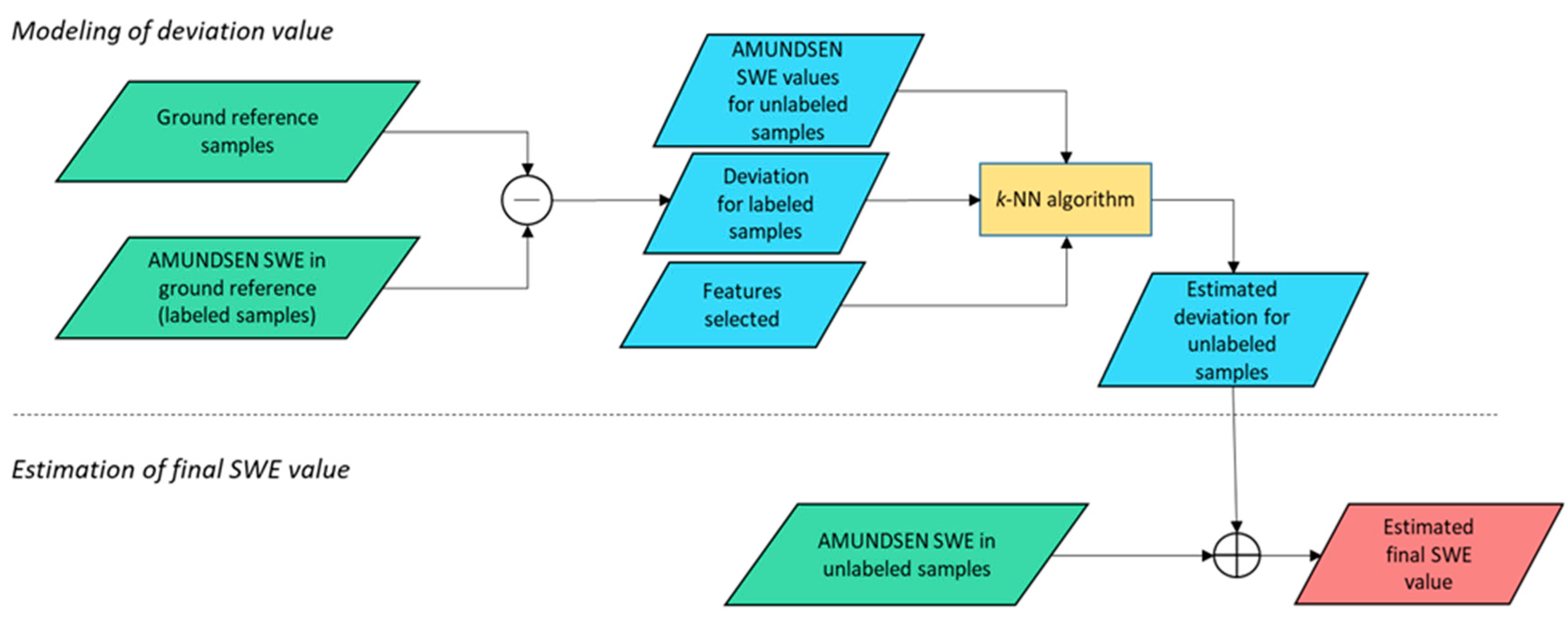
A feature-selection technique based on a genetic algorithm (GA) and a proper cost function has been used for each region (i.e., Tyrol, South Tryol and Trentino) of the study area, in order to assess which variables are more relevant for the estimation of the deviation term (target variable). The procedure adopts the approach presented in [50] and is shown in Figure 2.
A. Modeling of Deviation Value
This phase aims at computing the deviation values for unlabeled samples starting from the training dataset. For doing this, first the deviations for labeled samples are computed by calculating the difference between the AMUNDSEN SWE values and the respective ground samples. Then the deviation distribution is characterized in the feature space (consisting of the variables reported in Table 1). We adopted the Local Deviation Bias (LDB) strategy, which was tested to have better performance and describe the deviations more accurately with respect to the Global Deviation Bias (GDB) strategy [50]. LDB approach assumes that the AMUNDSEN model can provide different accuracies depending on the sample location in the feature space. In other words, the deviation locally changes in the space of the features and its value for an unlabeled sample is related to that of training samples located in the same portion of the feature space. The estimation of the deviations for the unlabeled samples is performed through the k-NN algorithm: For each unlabeled sample, the k-nearest labeled samples having the smallest distance in the feature space are identified and the deviation for the unlabeled sample is then calculated as the average deviation value of the k-nearest labeled samples.
The application of the k-NN algorithm to our study can be schematized as follows: given x i labeled samples of training dataset with i = 1 , ,   M , the output variable is represented by the deviation (between modelled and observed SWE), which is defined for each unlabeled sample x j as the average deviation value of the k-nearest labeled samples in the feature space:
δ ( x j ) = i = 1 M δ ( x i ) W ( x j , x i ) i = 1 M W ( x j , x i )
where W ( x j , x i ) is 0 or 1 depending on whether x i is among the k-NN’s of the unlabeled sample x j or not. This means that W ( x j , x i ) = 1 if x i is one of the k-NN’s of x j , and W ( x j , x i ) = 0 otherwise. An important question in this approach is how to select an optimal value of parameter k. In this study, we use the well-known rule of setting k as the square root of the half of the total number of reference samples [51].
B. Estimation of Final SWE Value
Once the deviations for all unlabeled samples ( δ i ^ ) are calculated, the final corrected SWE values ( S W E i A _ c o r r ) are obtained by adding them to the respective AMUNDSEN SWE value:
S W E i A _ c o r r = S W E i A + δ i ^
In other words, the estimate of SWE from AMUNDSEN simulations is corrected by the use of the deviation. The deviations differ from each other depending on the sample location in the feature space.

Validation Strategy

The above explained method has been applied for each region in the study area (Tyrol, South Tyrol and Trentino) separately as well as for the whole dataset, which includes all three regions. The method has been firstly validated by exploiting the ground data and then, once applied the method overall the study area, the generated SWE maps have been compared with binary MODIS snow maps. In the following, the two steps of validation and comparison are described.
- Validation with Ground Data
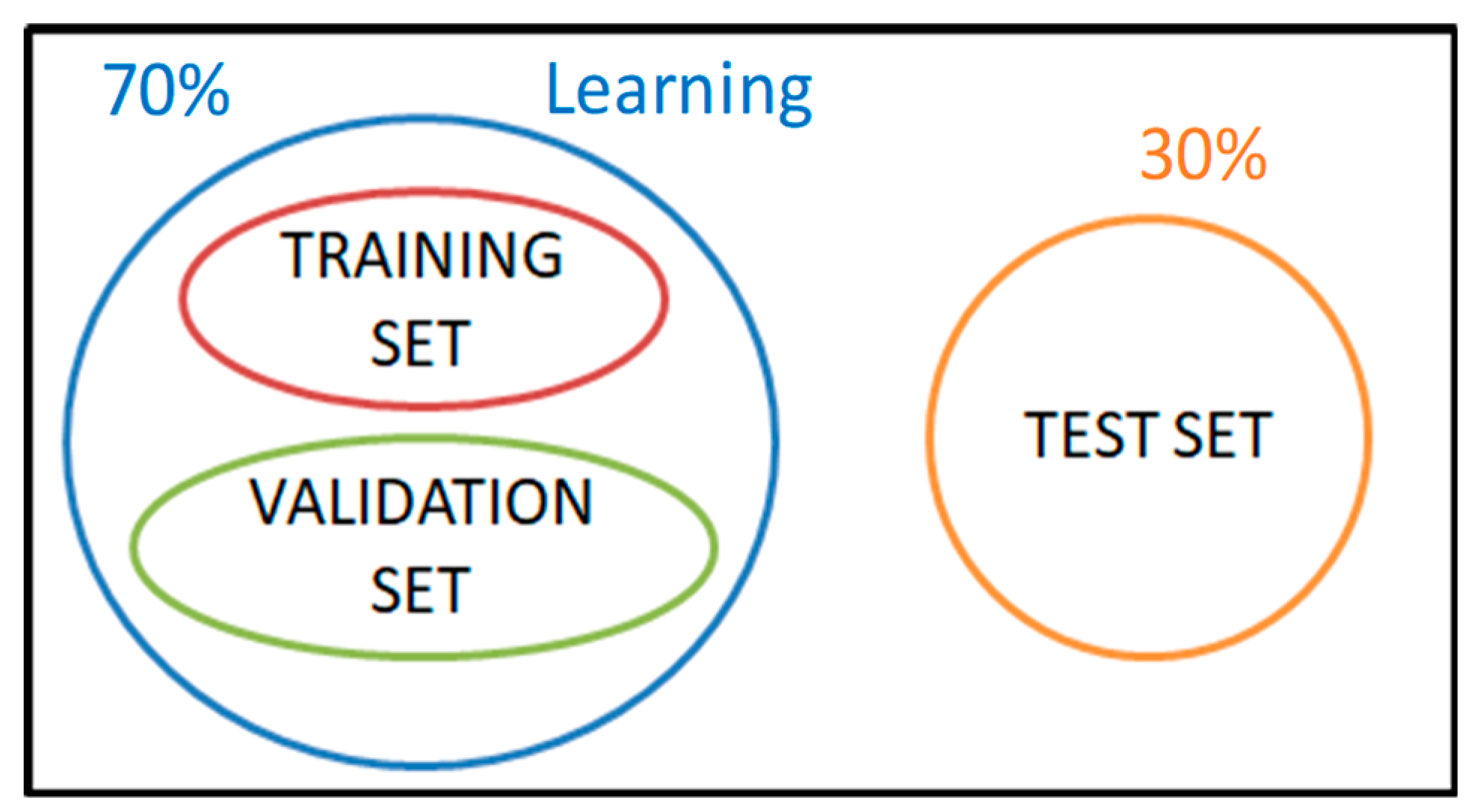
For each region and the whole dataset, the following procedure has been applied. The dataset has been divided into two independent datasets: The learning (70%) and test (30%) ones (Figure 3).
The 70% of learning dataset is used for generating the algorithm and is composed by a training and a validation set, used by applying a repeated 10-fold cross validation for 10 times. To ensure independence between datasets, as the deviation is time-correlated for each measurement point, the folds have been selected such that no points in the validation dataset are present in the training dataset even with a different time. This means that each time the algorithm uses 9 folds composed by certain measurement sites points as training dataset and the remaining one fold, which includes different measurement sites points, as validation dataset. Once the algorithm has been implemented, it has been tested on an independent test dataset, which include different measurement sites points with respect to the learning dataset, in order to evaluate the performances. The SWE values obtained have been compared with ground samples through the computation of some statistic metrics in order to evaluating the improvement achieved with the proposed method with respect to the AMUNDSEN simulations. The statistical metrics are the Root Mean Square Error (RMSE), the Mean Absolute Error (MAE), the determination coefficient ( R 2 ) and the bias. These metrics have been computes for both the training (as mean value of the repeated 10-fold cross validation results) and the test datasets in order to verify that the performance of the two datasets were consistent and without overfitting phenomena. Moreover, for test dataset, a scatterplot graph between estimated and ground samples together with the relative intercept and slope values has been reported.
- Comparison with Snow Cover Maps
The comparison with snow cover maps involves the information derived from the MODIS snow cover maps developed by Eurac Research, having a spatial resolution of 250 m [52,53]. In order to evaluate the agreement between the SWE maps from the AMUNDSEN simulations and the proposed method and the MODIS snow maps, a pixel-based analysis was performed. The SWE values of the maps are therefore converted into binary values. To this purpose, different values ranging between 20 mm and 50 mm [54] were tested and an acceptable SWE threshold was found to be equal to 50 mm, value for which it is very likely that a pixel is classified as snow-covered in the MODIS product. In this way the agreement between pixels in the SWE maps and those in the snow cover maps has been computed, by analyzing separately the two class (snow/no snow) and two different altitude belts.

3. Results and Discussion

In this section, we present analyses and results obtained with the proposed method. In Section 3.1 we show the comparison of SWE values modelled with AMUNDSEN. Then, in the Section 3.2, Section 3.3, Section 3.4, Section 3.5 and Section 3.6 we present the results obtained by the application of the proposed method.

3.1. Analysis of AMUNDSEN SWE Simulations

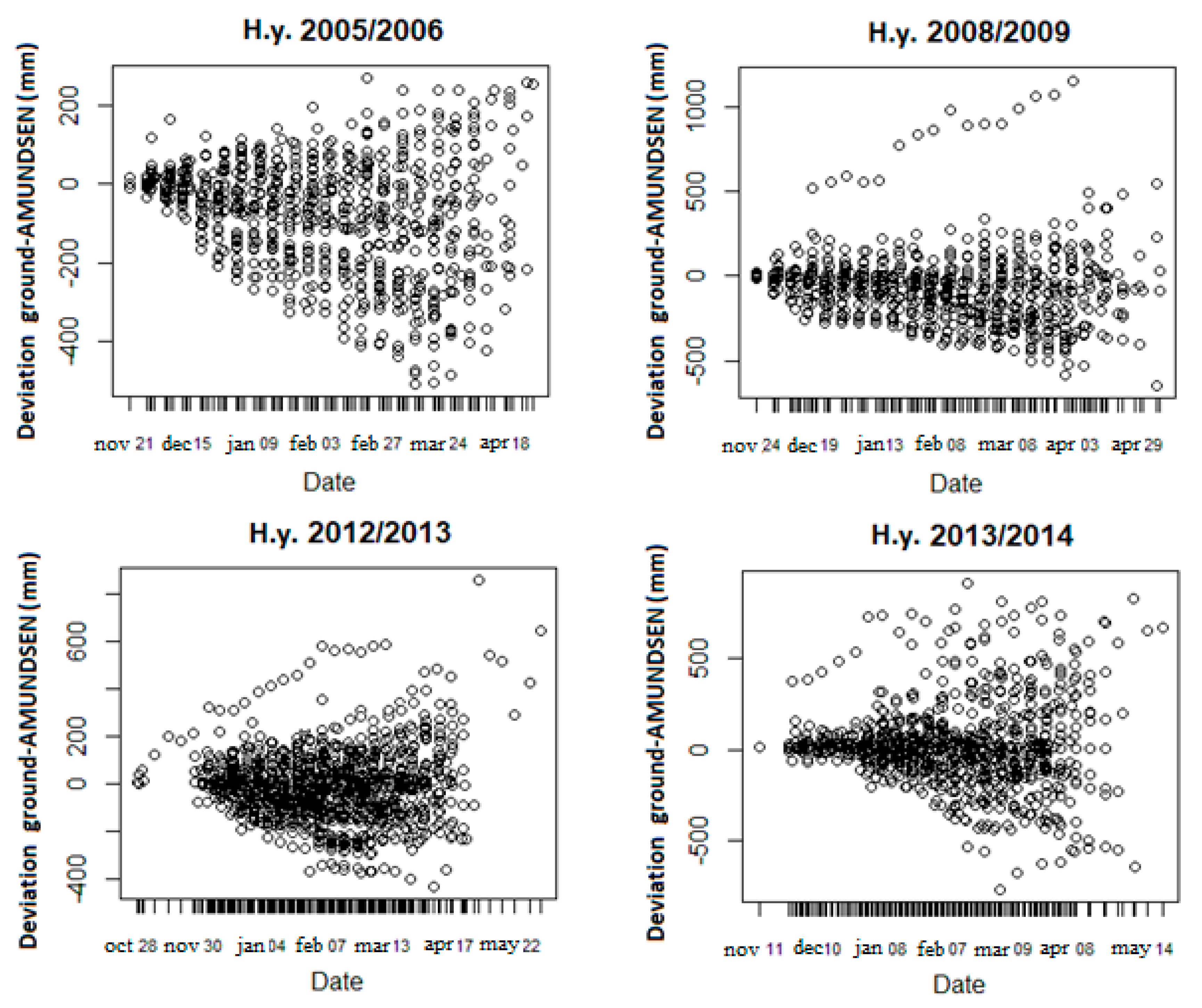
The analysis of the AMUNDSEN simulations helps to understand how the model results vary with respect to the period of the year, the altitude and the different regions included in the study area. This analysis will guide the identification of the training data samples that are representative of the area under study. Figure 4 shows the temporal evolution of the deviations between modelled and observed SWE for labeled samples. The main evidence, observed for all years, is the temporal increase of the spread in the deviations due to the cumulative nature in the SWE variable, so the deviation propagates in time. Table 2 shows the number of points for each year and the relative mean percentage error (MPE), calculated as the ratio between the deviation and the corresponding observed SWE value. The percentage error is a relative error and expresses how large the absolute error (namely deviation) is, compared to the total amount of the measured SWE. The lower maximum value of SWE observed in the hydrological year 2005–2006 is due to lower values of snow depth recorded in this year with respect to the other studied years. It is useful for comparing samples having differing size. In our case, SWE derived from ground measurements (hereafter also called “ground SWE”) can range from few mm up to around 1450 mm, as reported in the last column of Table 2.
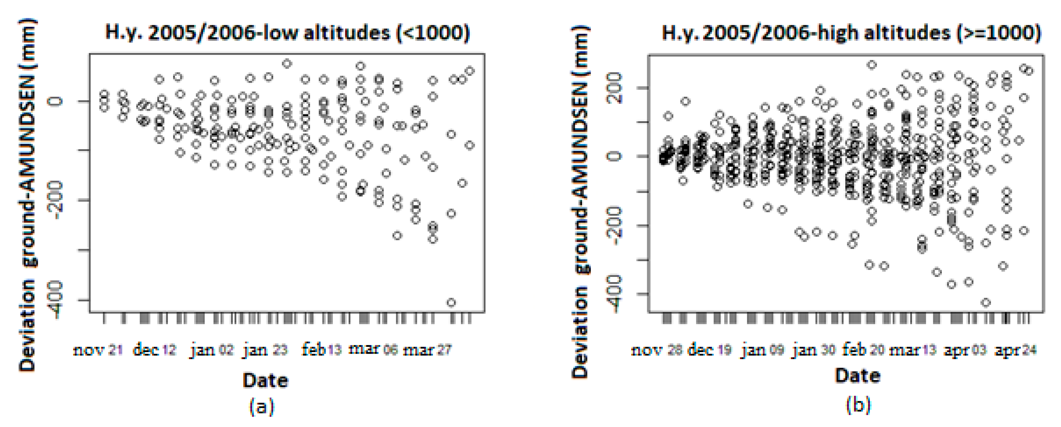
The analysis of the simulated SWE with respect to the altitude for the first study year 2005/2006 is shown in Figure 5 (the other years show similar behavior). By comparing the temporal evolution for altitudes lower than 1000 m and higher or equal to 1000 m, a different behavior can be observed: The distribution of deviation values for lower altitudes seems to be asymmetrical with respect to zero and the simulated SWE is higher (negative values) than the observed one (Figure 5a). This asymmetrical deviation distribution at low altitudes could be due to several reasons such as an error in estimation of the precipitation phase or gradient in the model [32,33], or the non-representativity of the observation sites at low altitudes.
Another factor to be considered is the thickness of the snowpack. At locations where the snowpack is shallower (typically at lower altitudes) and therefore with low SWE values, absolute underestimation cannot be high, since the SWE value is limited by a prediction of 0 mm. On the other side, there is no such limitation for the overestimation. This asymmetry in the deviation distribution does not appear at higher altitudes, where the snowpack is generally thicker. In this case the main evidence is the increasing temporal spread, as shown in Figure 5b.
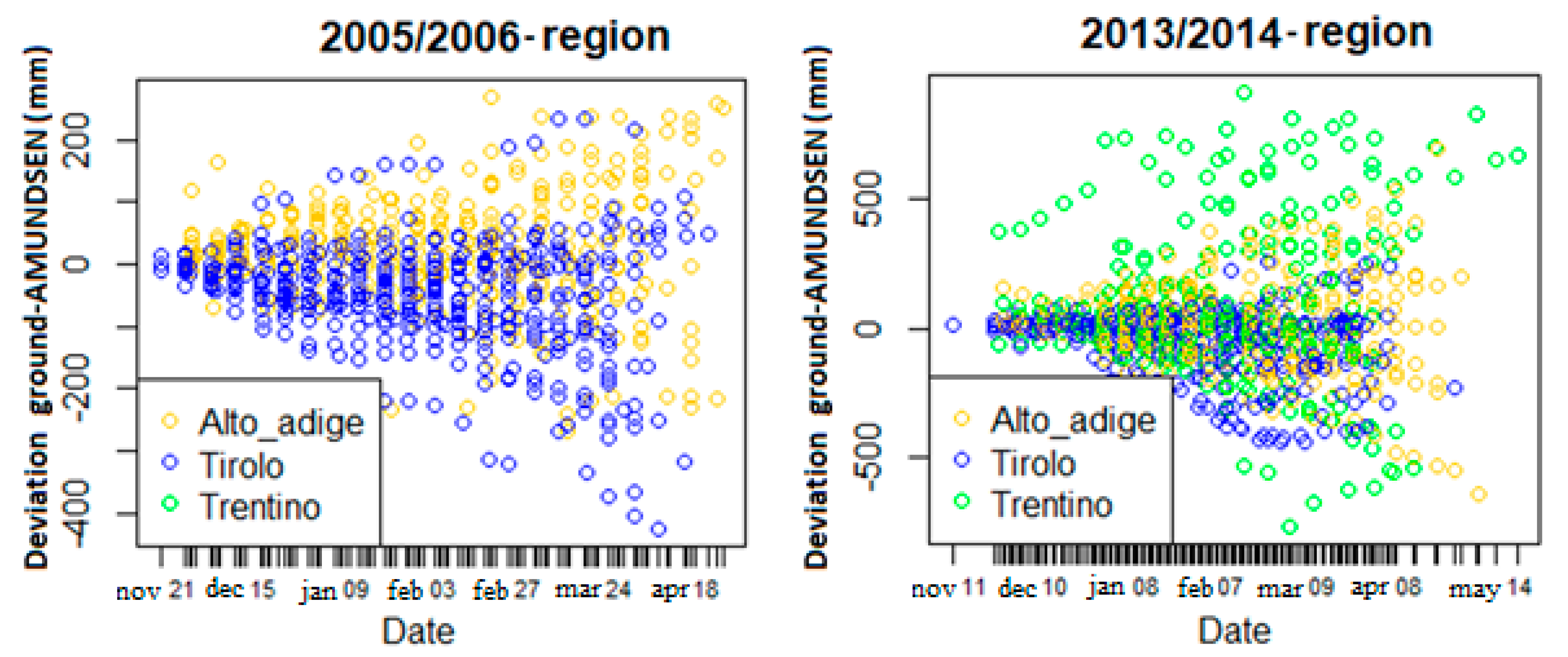
Finally, an analysis per region was performed. Figure 6 shows the deviation of the AMUNDSEN simulations from the ground values of local observations for Tyrol, South Tyrol and Trentino. In both graphs, the main remark is about the AMUNDSEN behavior for Tyrol area.
As for low altitudes, the deviations are asymmetric (again, by showing an overestimation of SWE by the snow model). Also in this case, this behavior could be ascribed to the measurement sites altitude. About 42% of measurement sites in Tyrol are located below 1000 m, while in Trentino and South Tyrol altitudes are always above 1000 m (in Trentino) and 1500 m (in South Tyrol). These preliminary analyses suggest different model performance depending on the period of the year and on the region of the study area. To evaluate the proposed method, we tested it on three different datasets, one per region, as well as on the entire dataset in order to identify differences in the performances that depend on the regional sampling.

3.2. Results: South Tyrol Dataset

For South Tyrol, 1270 observations are available. The k-NN algorithm was implemented by using the 70% of the sample, i.e., a sub-dataset of almost 900 samples. The target variable is the deviation, i.e., the difference between the AMUNDSEN simulation and the ground measurements derived SWE, and the feature space includes all variables indicated in Table 1. The resulting algorithm was then applied to the remaining 380 samples (test dataset) in order to evaluate the performance on a new and independent dataset. Once errors values are obtained, they are added to the corresponding simulated SWE in order to estimate its corrected value. Table 3 shows the performance in the estimation of SWE on both the training and the test data of the proposed method and the AMUNDSEN simulations.
The k-NN algorithm seems to halve both RMSE and MAE compared to the modelled SWE. However, the statistical metrics used are no relative errors and should be contextualized with respect to the range of respective absolute measured SWE, which in this case can reach very high values (up to 1450 mm).
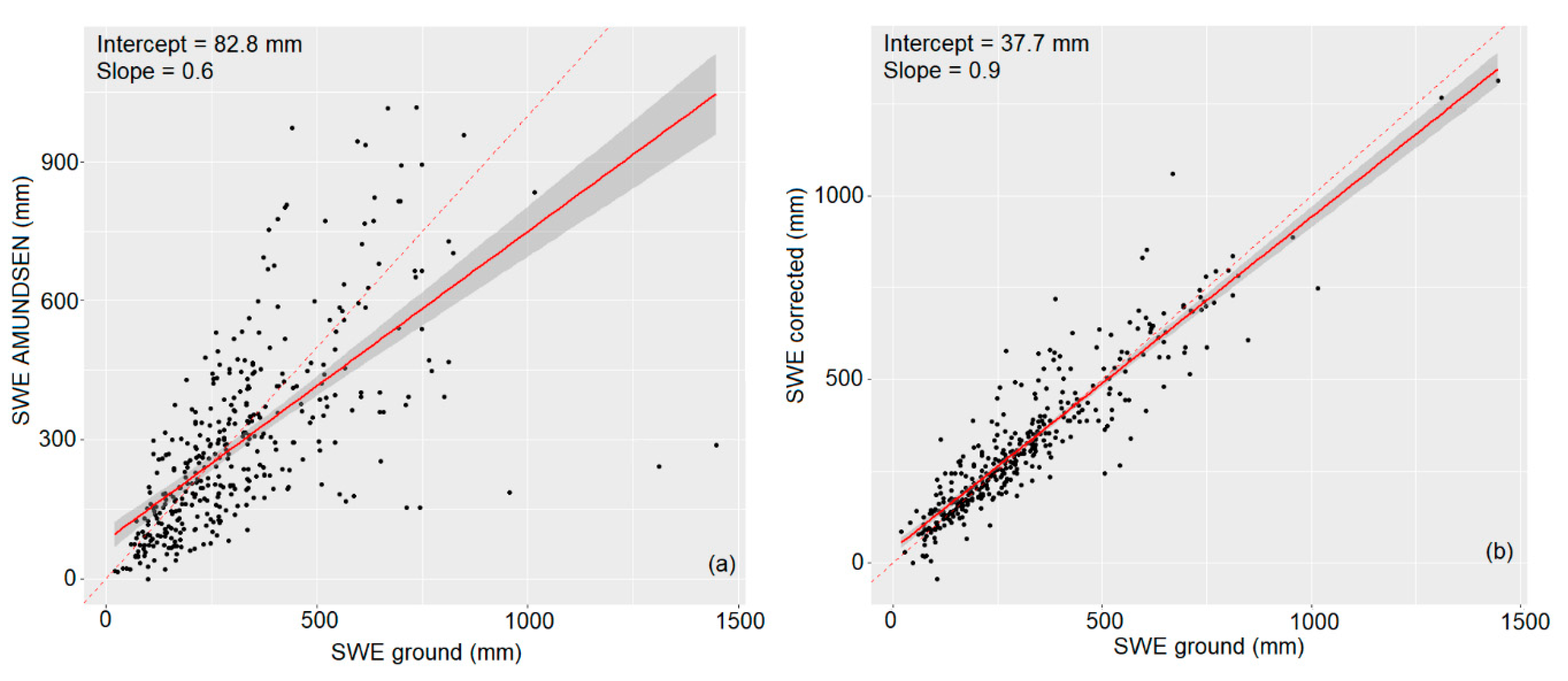
Figure 7 shows the comparison of scatterplots between observed SWE reference samples versus AMUNDSEN simulations (7a) and with the proposed method (7b). The absolute improvement of the SWE estimation is higher for higher observed values. Higher SWE values typically occur in the later season where the difference between the AMUNDSEN model results and the observations is larger.

3.3. Results: Tyrol Dataset

The analysis of the Tyrol dataset involves around 1470 observations. 70% of them (around 1030 samples) are used for implementing the algorithm with the same validation approach used for South Tyrol. Results relative to the remaining 30% of data (around 440 samples, test dataset) are shown together with the training dataset in Table 4. Also in this case, the proposed method provides a more accurate estimation in terms of MAE, RMSE and bias compared to the model simulation.
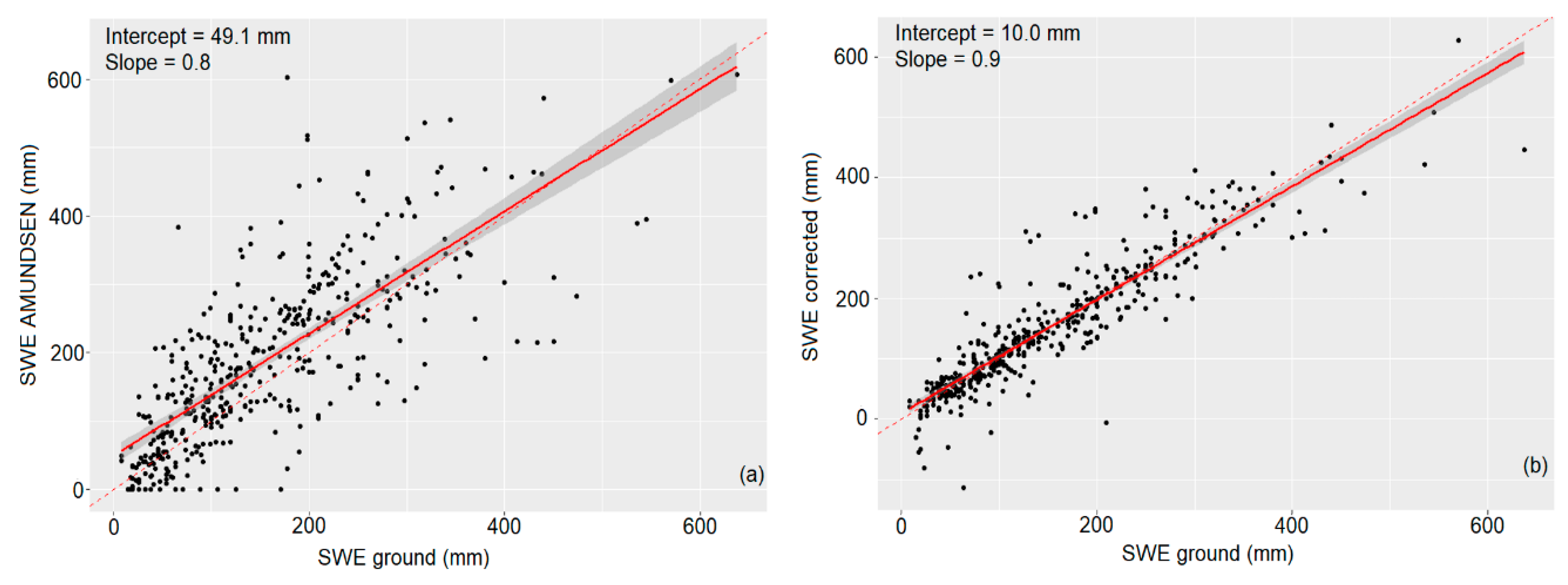
Figure 8 shows the scatterplots of estimated versus observed SWE values. Similar to the previous case of South Tyrol, the main result is that the proposed method reduces the difference between the two sources of SWE by increasing the slope of the regression line up to 0.9 and reducing the intercept value to 10 mm.

3.4. Results: Trentino Dataset

The third data set involves around 600 labeled observations. Also in this case, results are tested on 30% of the samples, i.e., around 180 data points. Table 5 reports the obtained values of MAE and RMSE together with the R-squared and the bias. Also in this case, the assumption that the deviation is varying depending on the sample location in the feature space leads to an improvement in the SWE estimation. The high RMSE of 240.7 mm for the AMUNDSEN simulations is probably due to the presence of numerous outliers and the small number of test points. Since the errors are squared before they are averaged, the RMSE gives a relatively high weight to large errors, by resulting impacted by the presence of outliers.
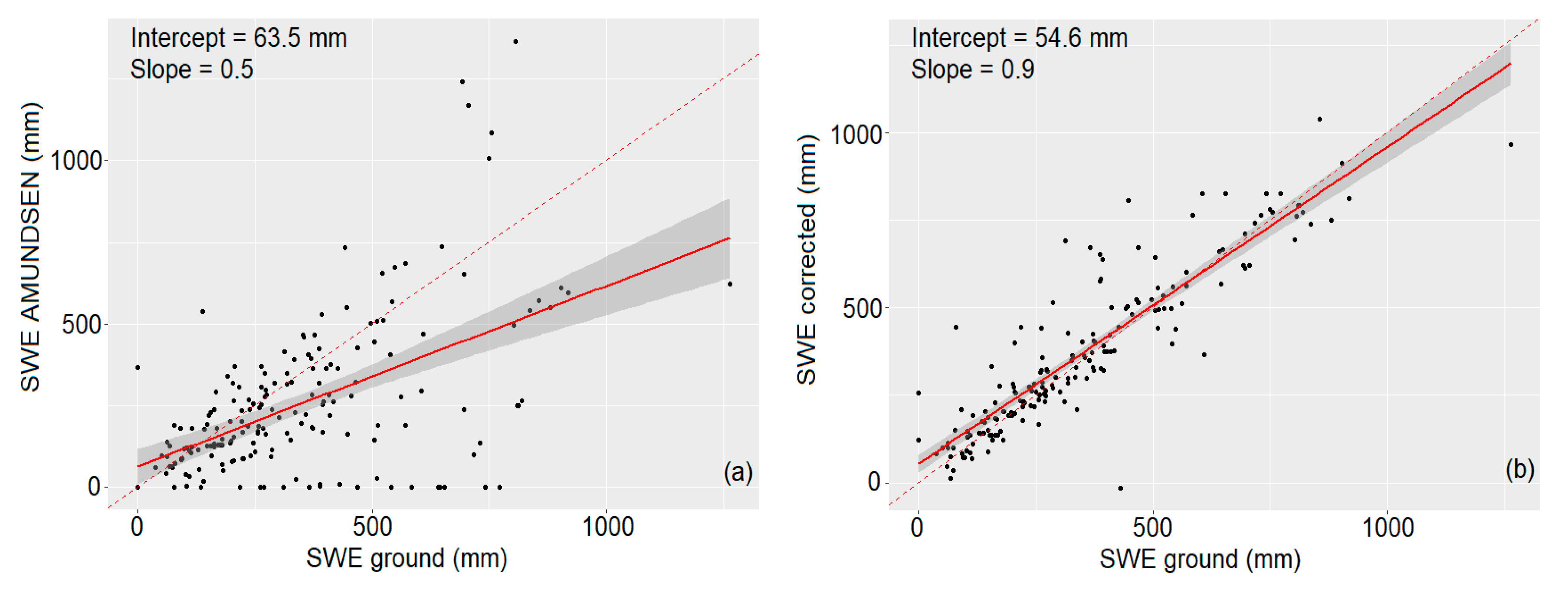
Figure 9 shows the proposed method based on the k-NN algorithm reduces the data spread and increases the slope of the regression line up to 0.9, while the RMSE sharply decreases to 102.8 mm.

3.5. Results: The Whole Dataset

The last analysis was conducted by using the whole dataset available, i.e., around 3300 observations, including the 4 years and the entire study area. 30% of the samples (i.e., around 1000 samples) were used for evaluating the performances of the proposed method. Table 6 reports the statistical metrics for the SWE estimations obtained with both the AMUNDSEN simulations and the proposed method. The performances for the whole data set are approximately equal to the mean performances achieved over the three regions separately.
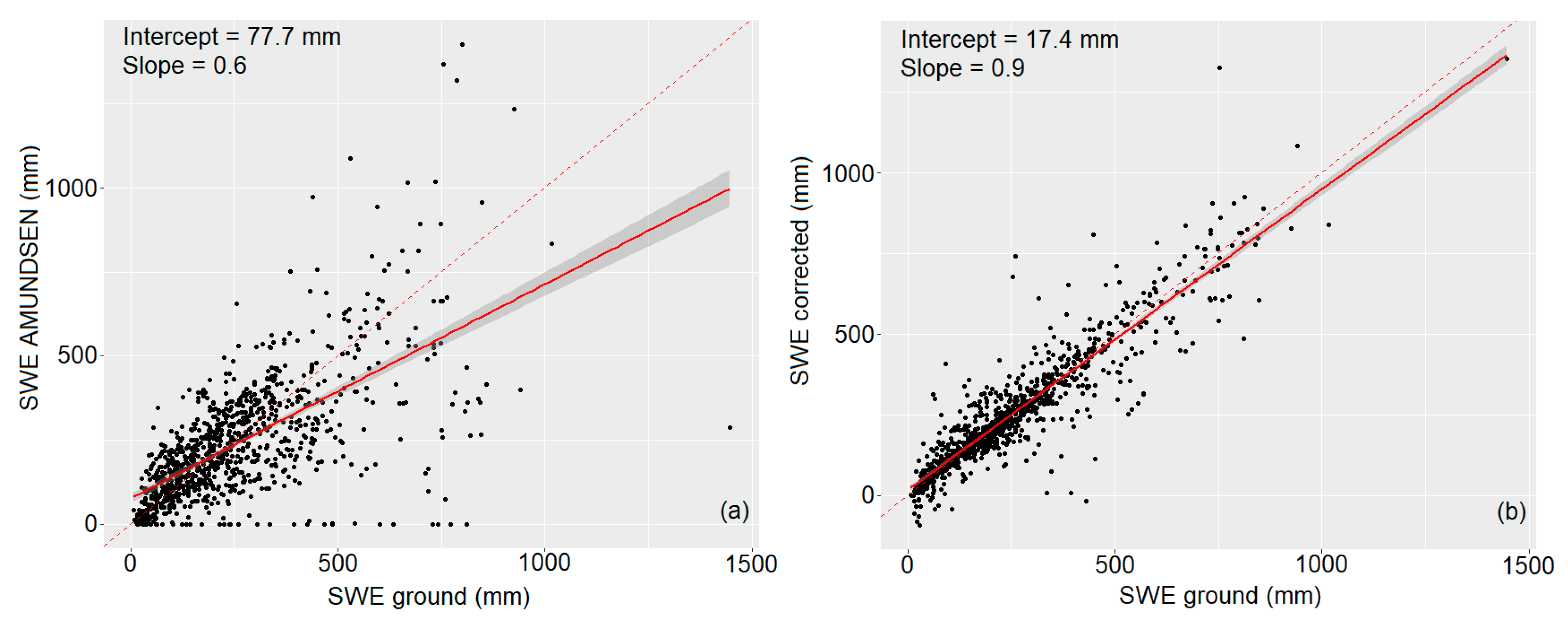
Figure 10 shows the scatterplots of simulated versus observed SWE, as well as a comparison of the proposed method results to the observations. The scatterplots confirm the results derived by quantitative analysis given in Table 6, pointing out an increase of the slope value and a corresponding decrease in the value of the square error RMSE for the proposed method.
Performances were then evaluated by analyzing different periods of the year and different altitudes. The test dataset was composed of around 600 measures from the winter period (i.e., November to February), and 400 points from spring (March to May). Around 200 of the test points are located below 1000 m, and the remaining 800 above 1000 m altitude. This disparity in test sample distribution with elevation is due to the fact that only 13.6% of the observation sites are located below 1000 m. Table 7 shows the RMSE and MAE in relation to the seasonal periods and altitude bands. As already mentioned in Section 3.1, the cumulative nature of SWE leads to a temporal increase of the deviations between the simulations and the results of the proposed method: From a value of RMSE of 124.8 mm in the winter period to a value of 200.8 mm in springtime. At low altitudes the uncertainty in the AMUNDSEN results is smaller than for high altitudes. This is probably due to the absolute nature of both RMSE and MAE and to the shallower snowpack at lower altitudes. This implies low SWE values and therefore lower absolute errors than for higher altitudes.

3.6. SWE Maps

Previous analyses provide the basis to create SWE maps for the entire study area. It was shown that applying the proposed method to the whole dataset results in a performance similar to the mean performance of the individual data sets. Furthermore, implementing a single algorithm for the whole study region reduces the computational cost significantly. For this reason, the generation of corrected SWE maps is based on the application of the proposed technique trained on the whole dataset. The resulting algorithm from the training procedure is then applied to the spatially distributed simulations of the Euregio region in order to generate a SWE map time series.
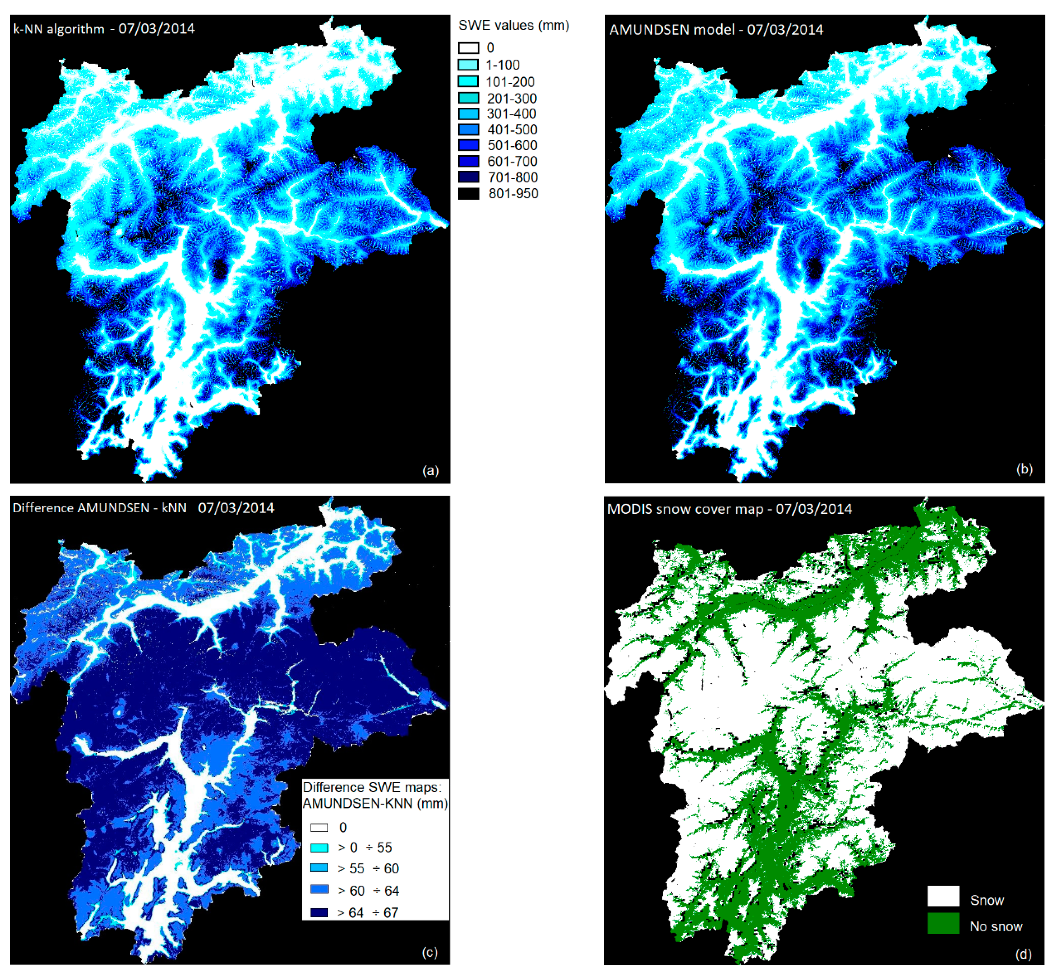
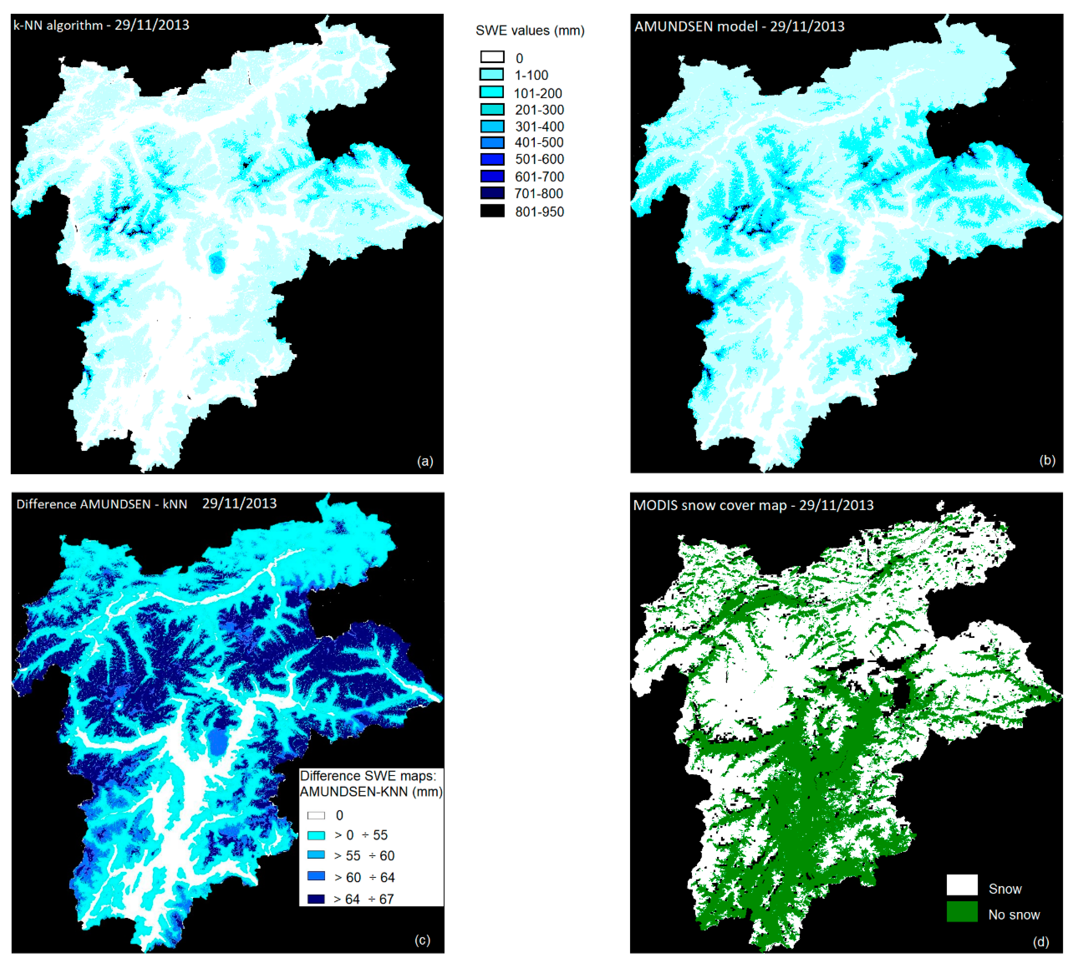
Figure 11 and Figure 12 show two examples of SWE maps obtained with the proposed method, compared to AMUNDSEN simulations and the MODIS snow cover maps developed by Eurac Research. The map in Figure 11 refers to an end-of-season situation (7 March 2014), while the maps in Figure 12 refer to a begin of the season (29 November 2013). In both cases, the proposed method shows lower SWE values compared to the AMUNDSEN simulations, especially for higher altitudes (more than 2000 m) where the difference between AMUNDSEN simulations and the SWE values estimated by the proposed method reach values up to 67 mm.
At the begin of the season, differences between the model and the proposed method results are more evident with respect to those of the end of the season, especially in the southern and in the northern part of the study area. The lower SWE values as evident in the map derived with the proposed method, in the southern part lead to an improved matching with the snow cover map derived by MODIS by better capturing the snow free areas.
Table 8 shows the pixel-based agreement in percentage between the SWE maps and the MODIS product. We can confirm the behavior found in Figure 11 and Figure 12, i.e., that the proposed method, in both cases, improves the estimation of snow-free areas, but shows lower values in the snow-covered areas, generally located at higher altitudes for the dates analyzed. An improvement could be achieved by integrating the dataset with more high-altitude points (in this study, only 15% is located above 2000 m) in order to provide more training data to the algorithm.

4. Conclusions

In this paper a new concept to improve the distributed estimation of snow water equivalent (SWE) is presented. The proposed method exploits a physically based model (AMUNDSEN), field observations, some topographic and auxiliary parameters and products from optical remote sensing for creating a time series of SWE maps for a region including Tyrol, South Tyrol and Trentino (Euregio area). Available ground reference samples are used for characterizing deviations of the snow model simulations affected, as any theoretical model, by uncertainties from approximations in the analytical formulation with respect to the observation. The hypothesis is that such deviations are varying depending on their location in the feature space. This behavior can be characterized by exploiting the properties of a specific k-Nearest Neighbor (k-NN) estimator, based on a “feature
Similarity” principle, to predict values of any new data point. Once the deviation is computed, it is added to the modelled SWE in order to obtain a corrected value.
Obtained results are promising with a significant improvement of performance: the new method in our data decreased, on average, the RMSE and the MAE from 154 to 75 mm and from 99 to 45 mm, respectively compared to the AMUNDSEN simulations. Furthermore, the slope of the regression line between estimated SWE and ground observations increases from 0.6 to 0.9 by reducing the data spread and the number of outliers.
In the approach presented in this study, two aspects are critical: The feature selection and the amount of observation samples. In this work, the feature selection in this work was performed through a genetic algorithm, by considering several variables supposed to be related to SWE computation. Different products from optical remote sensing were included in the feature selection, such as snow cover duration, snow cover fraction, different reflectance bands and the land surface temperature. The latter was found to be the only product relevant in our analysis. In particular, we exploited the mean surface temperature and the number of positive-temperature days, both computed on the last 30 days with respect to the date of ground acquisition. Certainly, many other parameters from remote sensing could be tested, such as products from radar sensors that are sensitive to the water presence in the snowpack [55]. A deeper and more extensive feature selection could for sure improve the results obtained.
Regarding the amount of ground observations, an improvement to the proposed approach could be achieved by increasing the dataset variability in the feature space. This could be done by acquiring, for example, ground measurements that are more differentiated in the feature space, such as different altitudes or different percentage of forest cover or slope.
We can conclude that the proposed approach effectively handles the variability of deviations between simulations and observations in the feature space and can be applied to other study areas and to other physically based snow models.
Author Contributions

Methodology, L.D.G., D.G., M.C., U.S., M.Z., L.B. and C.N.; validation, L.D.G.; formal analysis, L.D.G.; model simulations, D.G., U.S.; ground data curation, L.D.G.; writing—original draft preparation, L.D.G. and D.G.; writing—review and editing, D.G., M.C., U.S., M.Z., L.B. and C.N..

Funding

The research was supported by the project CRYOMON- SciPro: Improve the Science of Processes within the Cryosphere by Integrating Hydrological Modelling with Remote Sensing in a Multi-Level Data Fusion Approach—a Contribution to Cryosphere Monitoring in the Euregio Region. The project was funded by the Euregio Science Fund 1st call, project number IPN 10.

Acknowledgments

For ground data we gratefully acknowledge: The Hydrographic Service of Tyrol; Rudi Nadalet from the Autonomous Province of Bolzano, Agency for Civil Protection – Hydrographic Office (South Tyrol/ Alto Adige/ Südtirol); The Autonomous Province of Trento - Risk prevention service, Forecasting and planning office; Giacomo Bertoldi and Christian Brida from Alpine Environment Institute, Eurac Research, viale Druso, 1-39100 Bolzano, Italy, for providing the contact with the Autonomous Province of Trento and the data.

Conflicts of Interest

The authors declare no conflict of interest. The funders had no role in the design of the study; in the collection, analyses, or interpretation of data; in the writing of the manuscript, or in the decision to publish the results.

References

  1. Hock, R.; Rees, G.; Williams, M.W.; Ramirez, E. Contribution from glaciers and snow cover to runoff from mountains in different climates. Hydrol. Process. 2006, 20, 2089–2090. [Google Scholar] [CrossRef]
  2. Haberkorn, A. European Snow Booklet—An Inventory of Snow Measurements in Europe. EnviDat 2019. [Google Scholar] [CrossRef]
  3. Dressler, K.A.; Leavesley, G.H.; Bales, R.C.; Fassnacht, S.R. Evaluation of gridded snow water equivalent and satellite snow cover products for mountain basins in a hydrologic model. Hydrol. Process. 2006, 20, 673–688. [Google Scholar] [CrossRef]
  4. Fassnacht, S.R.; Dressler, K.A.; Bales, R.C. Snow water equivalent interpolation for the Colorado River Basin from snow telemetry (SNOTEL) data. Water Resour. Res. 2003, 39. [Google Scholar] [CrossRef] [Green Version]
  5. Molotch, N.P.; Fassnacht, S.R.; Bales, R.C.; Helfrich, S.R. Estimating the distribution of snow water equivalent and snow extent beneath cloud cover in the Salt–Verde River basin, Arizona. Hydrol. Process. 2004, 18, 1595–1611. [Google Scholar] [CrossRef]
  6. Elder, K.; Rosenthal, W.; Davis, R.E. Estimating the spatial distribution of snow water equivalence in a montane watershed. Hydrol. Process. 1998, 12, 1793–1808. [Google Scholar] [CrossRef]
  7. Molotch, N.P.; Bales, R.C. SNOTEL representativeness in the Rio Grande headwaters on the basis of physiographics and remotely sensed snow cover persistence. Hydrol. Process. 2006, 20, 723–739. [Google Scholar] [CrossRef]
  8. Neumann, N.N.; Derksen, C.; Smith, C.; Goodison, B. Characterizing local scale snow cover using point measurements during the winter season. Atmos. Ocean 2006, 44, 257–269. [Google Scholar] [CrossRef]
  9. Rice, R.; Bales, R.C. Embedded-sensor network design for snow cover measurements around snow pillow and snow course sites in the Sierra Nevada of California. Water Resour. Res. 2010, 46. [Google Scholar] [CrossRef]
  10. López-Moreno, J.I.; Fassnacht, S.R.; Beguería, S.; Latron, J.B.P. Variability of snow depth at the plot scale: Implications for mean depth estimation and sampling strategies. Cryosphere 2011, 5, 617–629. [Google Scholar] [CrossRef]
  11. Schneider, D.; Molotch, N.P. Real-time estimation of snow water equivalent in the Upper Colorado River Basin using MODIS-based SWE Reconstructions and SNOTEL data. Water Resour. Res. 2016, 52, 7892–7910. [Google Scholar] [CrossRef]
  12. Zheng, Z.; Molotch, N.P.; Oroza, C.A.; Conklin, M.H.; Bales, R.C. Spatial snow water equivalent estimation for mountainous areas using wireless-sensor networks and remote-sensing products. Remote Sens. Environ. 2018, 215, 44–56. [Google Scholar] [CrossRef]
  13. Schneider, D.; Molotch, N.P.; Deems, J.S. Estimating relationships between snow water equivalent, snow covered area, and topography to extend the Airborne Snow Observatory dataset. Cryosphere 2017. [Google Scholar] [CrossRef]
  14. Martinec, J.; Rango, A. Areal distribution of snow water equivalent evaluated by snow cover monitoring. Water Resour. Res. 1981, 17, 1480–1488. [Google Scholar] [CrossRef]
  15. Bair, E.H.; Rittger, K.; Davis, R.E.; Painter, T.H.; Dozier, J. Validating reconstruction of snow water equivalent in California’s Sierra Nevada using measurements from the NASA Airborne Snow Observatory. Water Resour. Res. 2016, 52, 8437–8460. [Google Scholar] [CrossRef]
  16. Brubaker, K.A.Y.E.; Rango, A.; Kustas, W. Incorporating radiation inputs into the snowmelt runoff model. Hydrol. Process. 1996, 10, 1329–1343. [Google Scholar] [CrossRef]
  17. Girotto, M.; Margulis, S.A.; Durand, M. Probabilistic SWE reanalysis as a generalization of deterministic SWE reconstruction techniques. Hydrol. Process. 2014, 28, 3875–3895. [Google Scholar] [CrossRef]
  18. Guan, B.; Molotch, N.P.; Waliser, D.E.; Jepsen, S.M.; Painter, T.H.; Dozier, J. Snow water equivalent in the Sierra Nevada: Blending snow sensor observations with snowmelt model simulations. Water Resour. Res. 2013, 49, 5029–5046. [Google Scholar] [CrossRef]
  19. Rittger, K.; Bair, E.H.; Kahl, A.; Dozier, J. Spatial estimates of snow water equivalent from reconstruction. Adv. Water Resour. 2016, 94, 345–363. [Google Scholar] [CrossRef] [Green Version]
  20. Painter, T.H.; Rittger, K.; McKenzie, C.; Slaughter, P.; Davis, R.E.; Dozier, J. Retrieval of subpixel snow covered area, grain size, and albedo from MODIS. Remote Sens. Environ. 2009, 113, 868–879. [Google Scholar] [CrossRef] [Green Version]
  21. Vuyovich, C.; Jacobs, J.M. Snowpack and runoff generation using AMSR-E passive microwave observations in the Upper Helmand Watershed, Afghanistan. Remote Sens. Environ. 2011, 115, 3313–3321. [Google Scholar] [CrossRef]
  22. Mizukami, N.; Perica, S. Towards improved snow water equivalent retrieval algorithms for satellite passive microwave data over the mountainous basins of western USA. Hydrol. Process. 2012, 26, 1991–2002. [Google Scholar] [CrossRef]
  23. Vuyovich, C.M.; Jacobs, J.M.; Daly, S.F. Comparison of passive microwave and modeled estimates of total watershed SWE in the continental United States. Water Resour. Res. 2014, 50, 9088–9102. [Google Scholar] [CrossRef] [Green Version]
  24. Chang, A.T.C.; Foster, J.L.; Hall, D.K. Effects of forest on the snow parameters derived from microwave measurements during the BOREAS winter field campaign. Hydrol. Process. 1996, 10, 1565–1574. [Google Scholar] [CrossRef]
  25. Nolin, A.W. Recent advances in remote sensing of seasonal snow. J. Glaciol. 2010, 56, 1141–1150. [Google Scholar] [CrossRef] [Green Version]
  26. Josberger, E.G.; Mognard, N.M. A passive microwave snow depth algorithm with a proxy for snow metamorphism. Hydrol. Process. 2002, 16, 1557–1568. [Google Scholar] [CrossRef]
  27. Durand, M.; Kim, E.J.; Margulis, S.A.; Molotch, N.P. A first-order characterization of errors from neglecting stratigraphy in forward and inverse passive microwave modeling of snow. IEEE Geosci. Remote Sens. Lett. 2011, 8, 730–734. [Google Scholar] [CrossRef]
  28. Sun, S.; Che, T.; Wang, J.; Li, H.; Hao, X.; Wang, Z.; Wang, J. Estimation and analysis of snow water equivalents based on C-band SAR data and field measurements. Arct. Antarct. Alp. Res. 2015, 47, 313–326. [Google Scholar] [CrossRef]
  29. Conde, V.; Nico, G.; Mateus, P.; Catalão, J.; Kontu, A.; Gritsevich, M. On the estimation of temporal changes of snow water equivalent by spaceborne SAR interferometry: A new application for the Sentinel-1 mission. J. Hydrol. Hydromech. 2019, 67, 93–100. [Google Scholar] [CrossRef]
  30. Rutter, N.; Essery, R.; Pomeroy, J.; Altimir, N.; Andreadis, K.; Baker, I.; Barr, A.; Bartlett, P.; Boone, A.; Deng, H.; et al. Evaluation of forest snow processes models (SnowMIP2). J. Geophys. Res. Space Phys. 2009, 114. [Google Scholar] [CrossRef] [Green Version]
  31. Zolezzi, G.; Bellin, A.; Bruno, M.C.; Maiolini, B.; Siviglia, A. Assessing hydrological alterations at multiple temporal scales: Adige River, Italy. Water Resour. Res. 2009, 45, 1–15. [Google Scholar] [CrossRef]
  32. Strasser, U. Die Modellierung der Gebirgsschneedecke im Nationalpark Berchtesgaden. In Modelling of the Mountain Snow Cover in the Berchtesgaden National Park; Berchtesgaden National Park research report, Nr. 55; The Berchtesgaden National Park: Berchtesgaden, Germany, 2008; ISSN 0172-0023. ISBN 978-3-922325-62-8. [Google Scholar]
  33. Essery, R. A Factorial Snowpack Model (FSM 1.0). Geosci. Model Dev. 2015, 8, 3867–3876. [Google Scholar] [CrossRef]
  34. Hanzer, F.; Helfricht, K.; Marke, T.; Strasser, U. Multi-level spatiotemporal validation of snow/ice mass balance and runoff modeling in glacierized catchments. Cryosphere 2016, 10, 1859–1881. [Google Scholar] [CrossRef]
  35. Renner, M.; Werner, M.G.F.; Rademacher, S.; Sprokkereef, E. Verification of ensemble flow forecasts for the River Rhine. J. Hydrol. 2009, 376, 463–475. [Google Scholar] [CrossRef]
  36. Charrois, L.; Cosme, E.; Dumont, M.; Lafaysse, M.; Morin, S.; Libois, Q.; Picard, G. On the assimilation of optical reflectances and snow depth observations into a detailed snow- pack model. Cryosphere 2016, 10, 1021–1038. [Google Scholar] [CrossRef]
  37. Günther, D.; Marke, T.; Essery, R.; Strasser, U. Uncertainties in Snowpack Simulations-Assessing the Impact of Model Structure, Parameter Choice and Forcing Data Error on Point-Scale Energy-Balance Snow Model Performance. Water Resour. Res. 2019, 55, 2779–2800. [Google Scholar] [CrossRef]
  38. Marks, D.; Winstral, A.; Reba, M.; Pomeroy, J.; Kumar, M. An evaluation of methods for determining during-storm precipitation phase and the rain/snow transition elevation at the surface in a mountain basin. Adv. Water Resour. 2013, 55, 98–110. [Google Scholar] [CrossRef]
  39. Strasser, U.; Corripio, J.; Brock, B.; Pellicciotti, F.; Burlando, P.; Funk, M. Spatial and Temporal Variability of Meteorological Variables at Haut Glacier d’Arolla (Switzerland) During the Ablation Season 2001: Measurements and Simulations. J. Geophys. Res. 2004, 109, D03103. [Google Scholar] [CrossRef]
  40. Fassnacht, S.R.; Dressler, K.A.; Hultstrand, D.M.; Bales, R.C.; Patterson, G. Temporal inconsistencies in coarse-scale snow water equivalent patterns: Colorado River Basin snow telemetry-topography regressions. Pirin. Rev. Ecol. Mont. 2012, 167, 165–185. [Google Scholar] [CrossRef] [Green Version]
  41. Erxleben, J.; Elder, K.; Davis, R. Comparison of spatial interpolation methods for estimating snow distribution in the Colorado Rocky Mountains. Hydrol. Process. 2002, 16, 3627–3649. [Google Scholar] [CrossRef]
  42. Snow Metamorphism. Available online: https://www.slf.ch/en/snow/snow-as-a-material/snow-metamorphism.html (accessed on 6 May 2019).
  43. Status for: Land Surface Temperature and Emissivity (MOD11). Available online: https://landval.gsfc.nasa.gov/ProductStatus.php?ProductID=MOD11 (accessed on 6 May 2019).
  44. Collection-6 MODIS Land Surface Temperature Products Users’ Guide. Available online: https://icess.eri.ucsb.edu/modis/LstUsrGuide/MODIS_LST_products_Users_guide_Collection-6.pdf (accessed on 6 May 2019).
  45. Earthdata. Available online: https://earthdata.nasa.gov/ (accessed on 6 May 2019).
  46. Martin, M.A.; Ghent, D.; Pires, A.C.; Göttsche, F.M.; Cermak, J.; Remedios, J.J. Comprehensive in situ validation of five satellite land surface temperature data sets over multiple stations and years. Remote Sens. 2019, 11, 479. [Google Scholar] [CrossRef]
  47. Oesch, D.; Wunderle, S.; Hauser, A. Snow surface temperature from AVHRR as a proxy for snowmelt in the Alps. In Proceedings of the EARSeL-LISSIG-Workshop Observing our Cryosphere from Space, Bern, Switzerland, 11–13 March 2002. [Google Scholar]
  48. Colombo, R.; Garzonio, R.; Di Mauro, B.; Dumont, M.; Tuzet, F.; Cogliati, S.; Pozzi, G.; Maltese, A.; Cremonese, E. Introducing Thermal Inertia for Monitoring Snowmelt Processes With Remote Sensing. Geophys. Res. Lett. 2019, 46, 4308–4319. [Google Scholar] [CrossRef]
  49. Associazione Interregionale di coordinamento e documentazione per i problemi inerenti alla neve e alle valanghe – Modelli AINEVA per i rilievi. Available online: https://www.aineva.it/modelli-aineva-per-i-rilievi/ (accessed on 14 May 2019).
  50. Castelletti, D.; Pasolli, L.; Bruzzone, L.; Notarnicola, C.; Demir, B. A novel hybrid method for the correction of the theoretical model inversion in bio/geophysical parameter estimation. IEEE Trans. Geosci. Remote Sens. 2016, 54, 4764–4774. [Google Scholar] [CrossRef]
  51. Mardia, K.V.; Kent, J.T.; Bibby, J.M. Multivariate Analysis; Academic Press: New York, NY, USA, 1979. [Google Scholar]
  52. Notarnicola, C.; Duguay, M.; Moelg, N.; Schellenberger, T.; Tetzlaff, A.; Monsorno, R.; Costa, A.; Steurer, C.; Zebisch, M. Snow cover maps from MODIS images at 250 m resolution, Part 1: Algorithm description. Remote Sens. 2013, 5, 110–126. [Google Scholar] [CrossRef]
  53. Notarnicola, C.; Duguay, M.; Moelg, N.; Schellenberger, T.; Tetzlaff, A.; Monsorno, R.; Costa, A.; Steurer, C.; Zebisch, M. Snow cover maps from MODIS images at 250 m resolution, Part 2: Validation. Remote Sens. 2013, 5, 1568–1587. [Google Scholar] [CrossRef]
  54. Gascoin, S.; Hagolle, O.; Huc, M.; Jarlan, L.; Dejoux, J.F.; Szczypta, C.; Marti, R.; Sánchez, R. A snow cover climatology for the Pyrenees from MODIS snow products. Hydrol. Earth Syst. Sci. 2015, 19, 2337–2351. [Google Scholar] [CrossRef] [Green Version]
  55. Lemmetyinen, J.; Derksen, C.; Rott, H.; Macelloni, G.; King, J.; Schneebeli, M.; Wiesmann, A.; Leppänen, L.; Kontu, A.; Pulliainen, J. Retrieval of Effective Correlation Length and Snow Water Equivalent from Radar and Passive Microwave Measurements. Remote Sens. 2018, 10, 170. [Google Scholar] [CrossRef]
Figure 1. Study area: Tyrol (Austria), South Tyrol (Italy) and Trentino (Italy) and location of the measurement sites.
Remotesensing 11 02033 g001
Figure 2. Flow chart of the proposed method for SWE retrieval.
Remotesensing 11 02033 g002
Figure 3. Separation of dataset for generating and testing the k-NN algorithm.
Remotesensing 11 02033 g003
Figure 4. Temporal evolution of the deviation of AMUNDSEN model from ground measurements derived SWE for the 4 years analyzed.
Remotesensing 11 02033 g004
Figure 5. Deviation evolution with respect to the altitude, for low altitudes, <1000 meters (a) and for higher altitudes, >=1000 meters (b).
Remotesensing 11 02033 g005
Figure 6. Analysis per region. For 2005/2006 no data from Trentino are available.
Remotesensing 11 02033 g006
Figure 7. Regression scatterplot for South Tyrol dataset: simulated SWE vs observation (a) and corrected SWE vs observation (b). The dashed line represents the 1:1 line.
Remotesensing 11 02033 g007
Figure 8. Regression scatterplot for Tyrol dataset: Simulated SWE vs observation (a) and corrected SWE vs observation (b). The dashed line represents the 1:1 line.
Remotesensing 11 02033 g008
Figure 9. Regression scatterplot for Trentino dataset: Simulated SWE vs observation (a) and corrected SWE vs observation (b). The dashed line represents the 1:1 line.
Remotesensing 11 02033 g009
Figure 10. Regression scatterplot for the whole dataset: Simulated SWE vs observation (a) and corrected SWE vs observation (b). The dashed line represents the 1:1 line.
Remotesensing 11 02033 g010
Figure 11. March 7th, 2014: (a) SWE map generated by the proposed method and (b) by the AMUNDSEN simulations. (c) is the difference between the two products and (d) the snow cover map product by MODIS.
Remotesensing 11 02033 g011
Figure 12. November 29th, 2013: (a) SWE map generated by the proposed method and (b) by the AMUNDSEN simulations. (c) is the difference between the two products and (d) the snow cover map product by MODIS.
Remotesensing 11 02033 g012
Table 1. Features selected for implementing the k-NN algorithm (above); number of SWE ground samples available for each region (below).
Feature NameFeature Description
AltitudeMeasurement site altitude
Geographic coordinatesMeasurement site latitude and longitude
Forest coveragePercentage of pixel (containing measurement site) covered by forest
SlopePixel slope
AspectPixel aspect
Day of the year (DOY)DOY rescaled with respect to the start of hydrological year (the day number 1 is the 1st of October).
SWE value from AMUNDSENSWE value from AMUNDSEN corresponding to location and date of each ground measurement.
SWE climatologyCalculated as average SWE value (from AMUNDSEN) on the other years (10 years).
SWE quality measure (CV)Coefficient of Variation (standard deviation divided by the mean) on ensemble SWE simulations.
Land Surface Temperature (LST)Mean daily LST calculated on previous month and number of days in previous month having positive temperatures.
Region# of SWE ground samples
South Tyrol1270
Tyrol1467
Trentino605
Table 2. Number of samples and Mean Percentage Error (MPE) for each considered study year.
Hydrological YearNumber of SamplesMean Percentage ErrorMin–Max Values of Observed SWE (mm)
2005–200676023.5%4–512
2008–200970818.6%15–1446
2012–201310179.6%8–1264
2013–20148565.2%5–997
Table 3. Estimation performance obtained with AMUNDSEN simulation and with proposed method on the test dataset of South Tyrol.
RegionDatasetEstimation MethodRMSE (mm)MAE (mm) R 2 Bias
South TyrolTrainingAMUNDSEN166.3111.20.437.5
Proposed method77.249.50.81.4
TestAMUNDSEN167.7109.70.433.8
Proposed method80.953.40.82.5
Table 4. Estimation performance obtained with AMUNDSEN simulation and with proposed method on the test dataset relative to Tyrol.
RegionDatasetEstimation MethodRMSE (mm)MAE (mm) R 2 Bias
TyrolTrainingAMUNDSEN89.465.10.634.8
Proposed method39.426.20.90.7
TestAMUNDSEN88.464.90.632.6
Proposed method44.828.10.81.3
Table 5. Estimation performance obtained with both the AMUNDSEN simulation and the proposed method on the test dataset relative to Trentino.
RegionDatasetEstimation MethodRMSE (mm)MAE (mm) R 2 Bias
TrentinoTrainingAMUNDSEN251.4170.80.3−82.6
Proposed method101.563.20.812.9
TestAMUNDSEN240.7162.70.3−91.0
Proposed method102.865.30.818.6
Table 6. Estimation performance obtained with both the AMUNDSEN simulation and the proposed method on the test dataset relative to entire study area.
Region DatasetEstimation MethodRMSE (mm)MAE (mm) R 2 Bias
EuregioTraining AMUNDSEN163.2103.40.4−14.1
Proposed method70.041.60.81.3
TestAMUNDSEN153.798.70.4−12.2
Proposed method75.345.00.8−1.7
Table 7. Performance obtained with both the AMUNDSEN simulations and the proposed method by dividing the test dataset in two seasonal periods and two altitude bands.
PeriodEstimation MethodRMSE (mm)MAE (mm)
WinterAMUNDSEN124.877.9
Proposed method64.537.0
SpringAMUNDSEN200.8142.0
Proposed method93.861.4
AltitudeEstimation MethodRMSE (mm)MAE (mm)
Low altitudes (≤1000 m)AMUNDSEN89.368.1
Proposed method55.532.7
High altitudes (>1000 m)AMUNDSEN163.0104.5
Proposed method78.447.3
Table 8. Agreement between MODIS snow maps and SWE maps estimated with AMUNDSEN and with proposed method.
07/03/2014Estimation methodAgreement with MODIS no snowAgreement with MODIS snow
AMUNDSEN53%44% (≤1000 m)97%1% (≤1000 m)
9% (>1000 m)96% (>1000 m)
Proposed method (k-NN)61%46% (≤1000 m)93%1% (≤1000 m)
15% (>1000 m)92% (>1000 m)
29/11/2013Estimation methodAgreement with MODIS no snowAgreement with MODIS snow
AMUNDSEN86%34% (≤1000 m)59%0% (≤1000 m)
52% (>1000 m)59% (>1000 m)
Proposed method (k-NN)98%34% (≤1000 m)29%0% (≤1000 m)
64% (>1000 m)29% (>1000 m)