Detecting Forest Changes Using Dense Landsat 8 and Sentinel-1 Time Series Data in Tropical Seasonal Forests


Abstract

1. Introduction
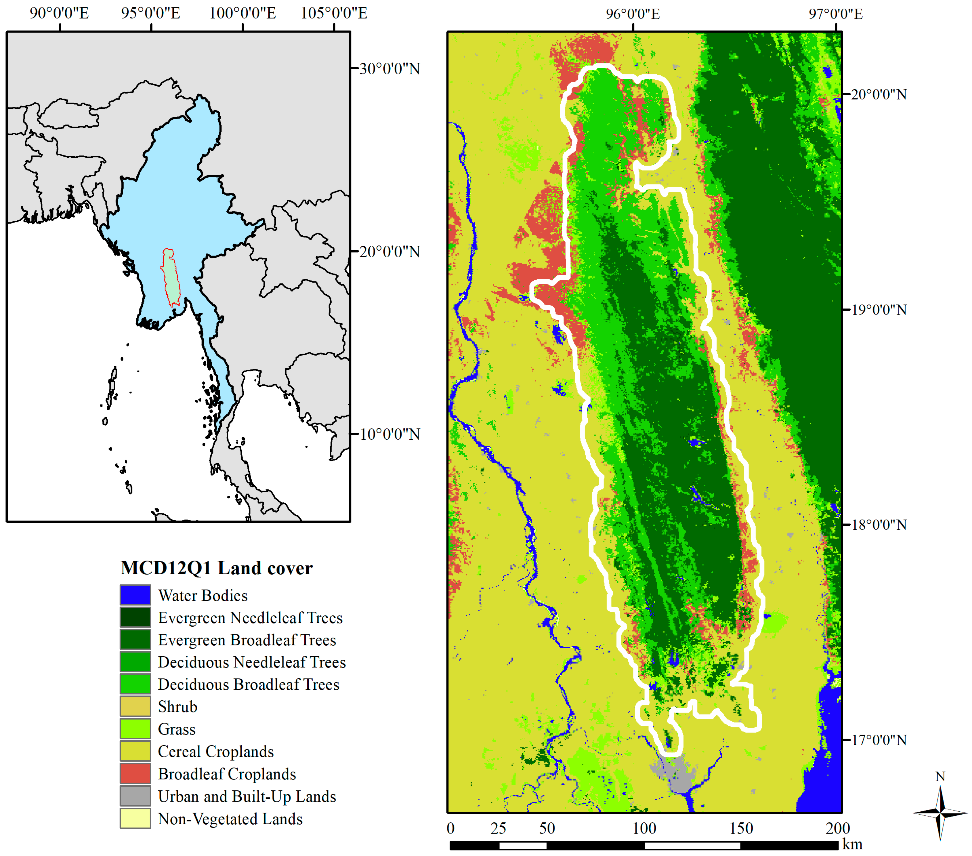
2. Study Area
3. Data and Methods
3.1. Preprocessing of Landsat 8, Sentinel-1 and Topographic Data
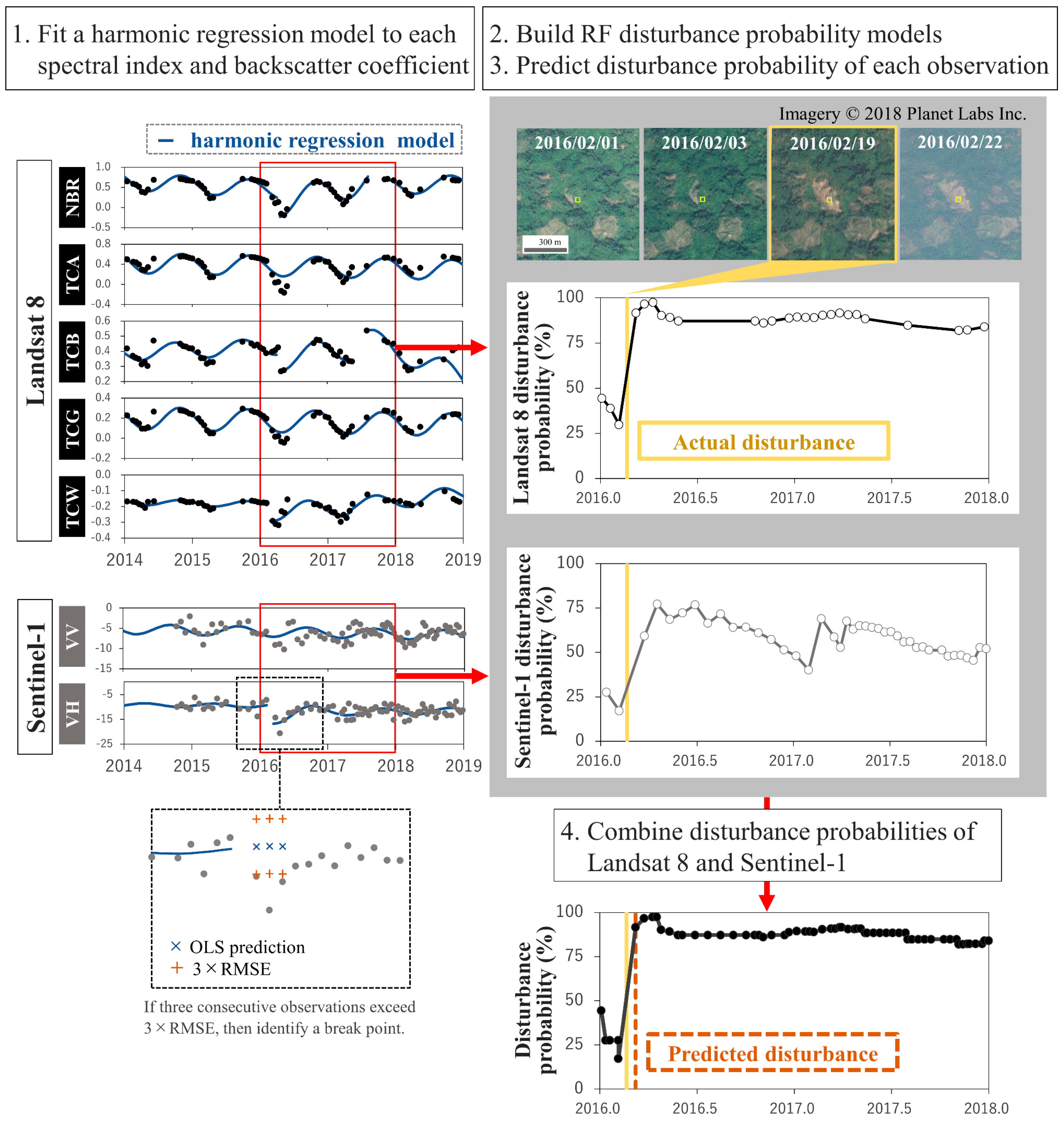
3.2. RF Disturbance Probability Models for Landsat 8 and Sentinel-1
3.3. Detection of Forest Disturbance Using Time Series Disturbance Probabilities
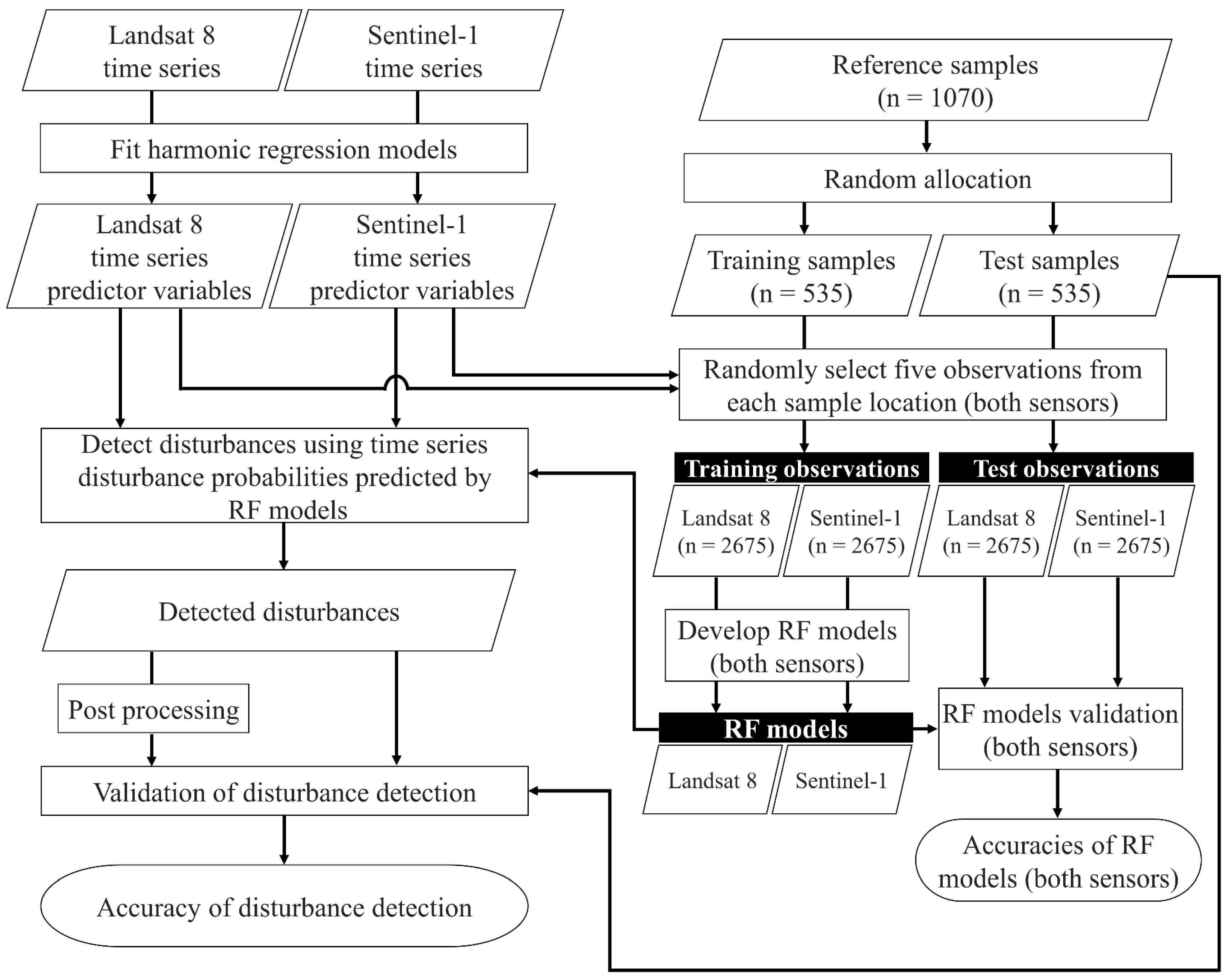
3.4. Collection of Reference Samples
3.5. Validation
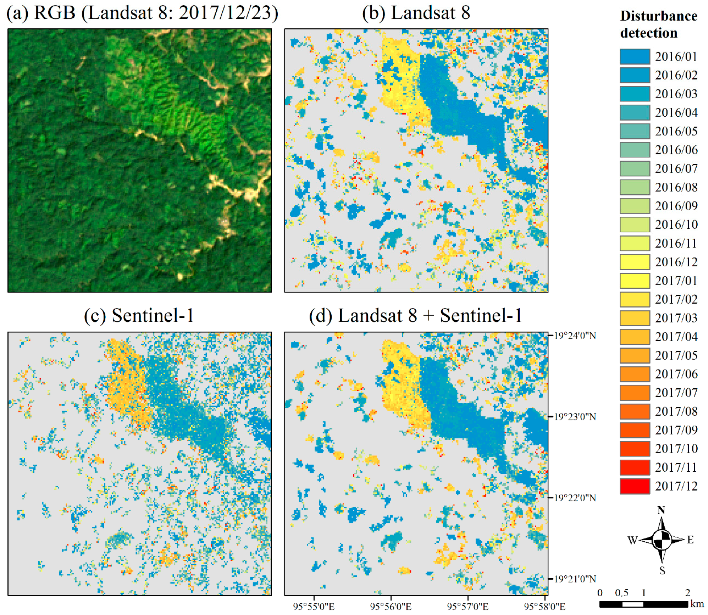
4. Results
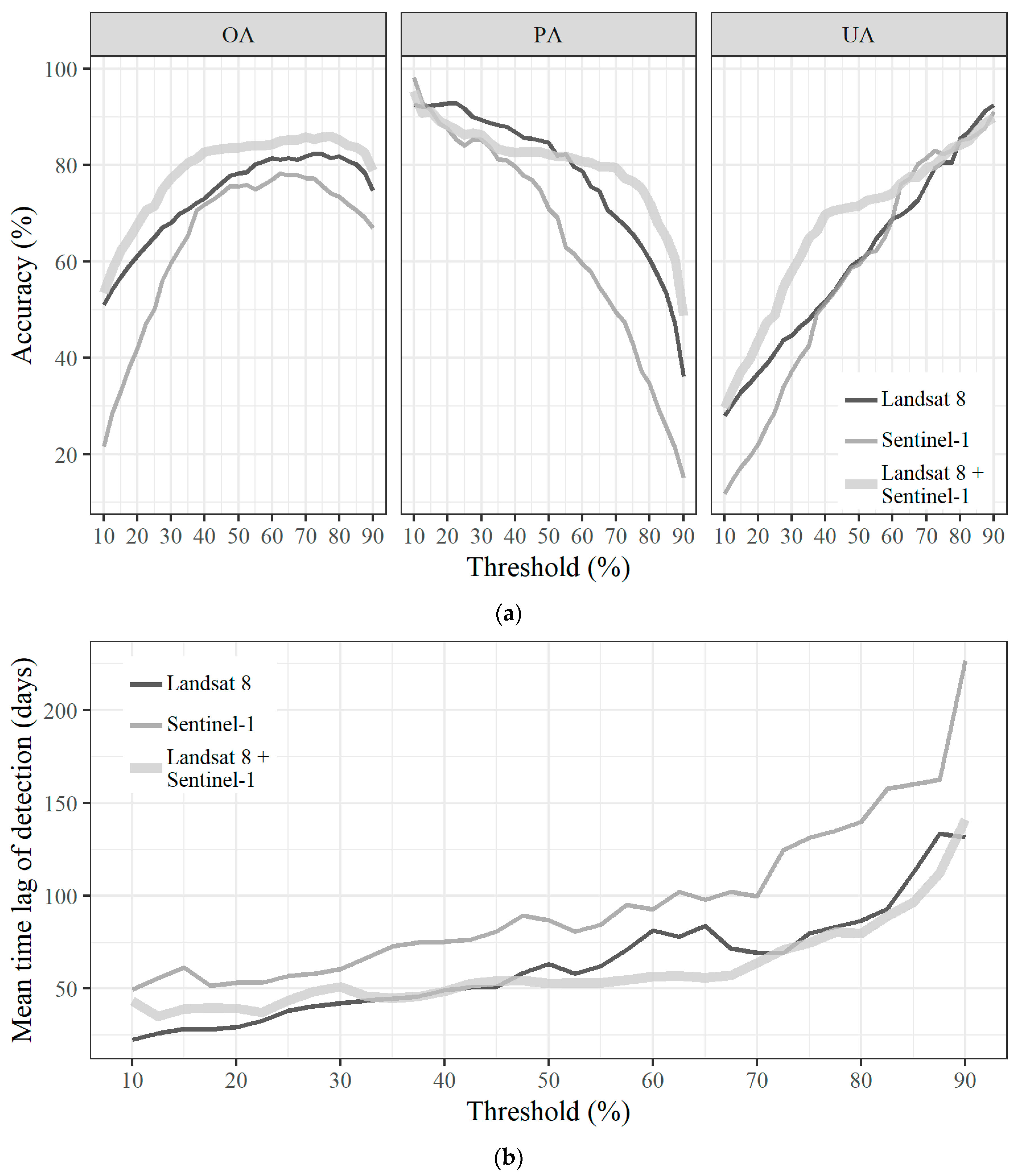
4.1. Accuracy of RF Disturbance Probability Models
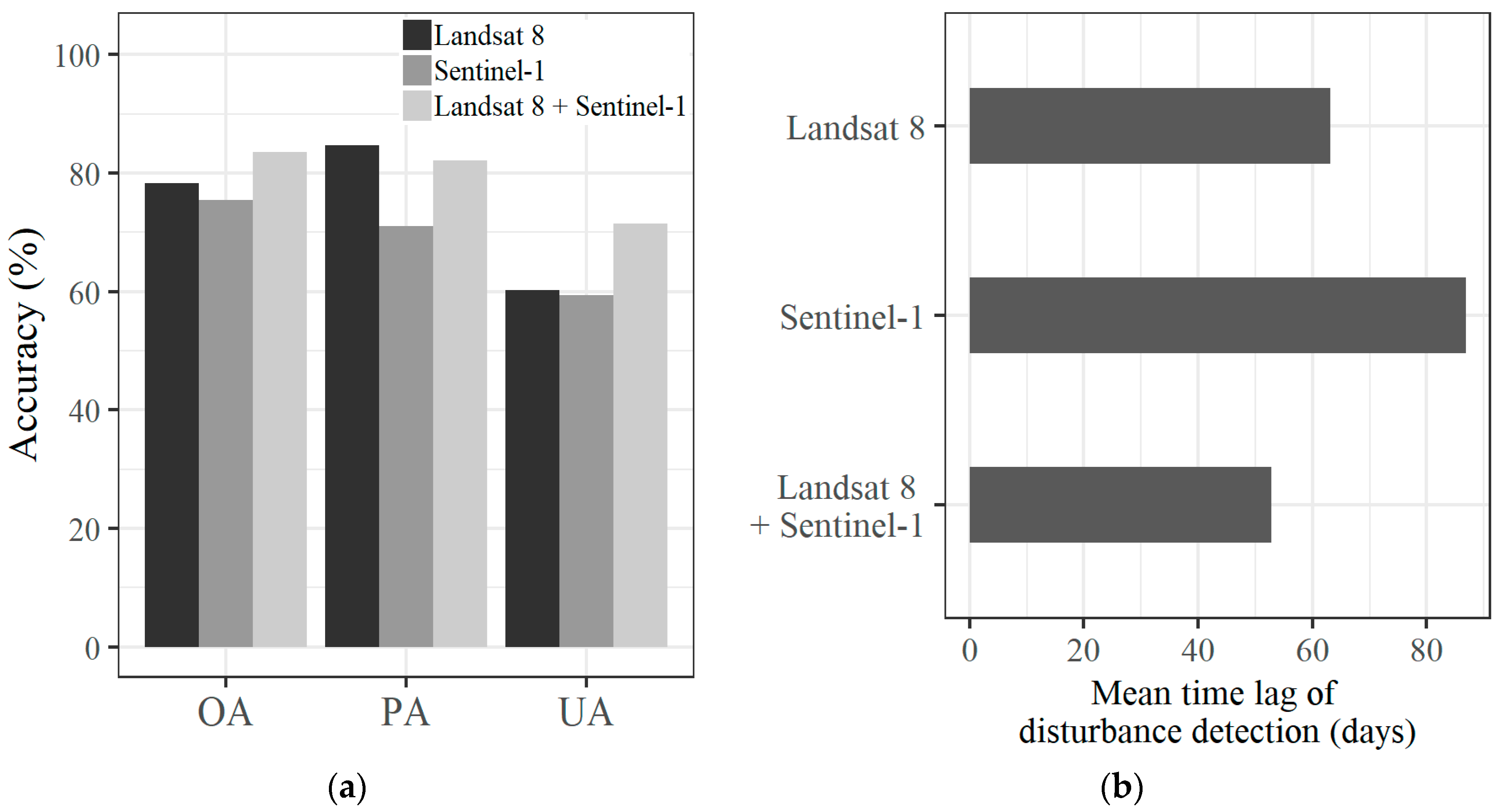
4.2. Accuracy of Disturbance Detection Using Time Series Disturbance Probabilities
5. Discussion
6. Conclusions
Author Contributions
Funding
Acknowledgments
Conflicts of Interest
References
- Kennedy, R.E.; Andréfouët, S.; Cohen, W.B.; Gómez, C.; Griffiths, P.; Hais, M.; Healey, S.P.; Helmer, E.H.; Hostert, P.; Lyons, M.B.; et al. Bringing an ecological view of change to landsat-based remote sensing. Front. Ecol. Environ. 2014, 12, 339–346. [Google Scholar] [CrossRef]
- Brosofske, K.D.; Froese, R.E.; Falkowski, M.J.; Banskota, A. A Review of Methods for Mapping and Prediction of Inventory Attributes for Operational Forest Management. For. Sci. 2014, 60, 733–756. [Google Scholar] [CrossRef]
- Roy, D.P.; Wulder, M.A.; Loveland, T.R.; Carabajal, C.C.; Allen, R.G.; Anderson, M.C.; Helder, D.; Irons, J.R.; Johnson, D.M.; Kennedy, R.; et al. Landsat-8: Science and product vision for terrestrial global change research. Remote Sens. Environ. 2014, 145, 154–172. [Google Scholar] [CrossRef]
- Wulder, M.A.; White, J.C.; Loveland, T.R.; Woodcock, C.E.; Belward, A.S.; Cohen, W.B.; Fosnight, E.A.; Shaw, J.; Masek, J.G.; Roy, D.P. The global Landsat archive: Status, consolidation, and direction. Remote Sens. Environ. 2016, 185, 271–283. [Google Scholar] [CrossRef]
- Wulder, M.A.; Loveland, T.R.; Roy, D.P.; Crawford, C.J.; Masek, J.G.; Woodcock, C.E.; Allen, R.G.; Anderson, M.C.; Belward, A.S.; Cohen, W.B.; et al. Current status of Landsat program, science, and applications. Remote Sens. Environ. 2019, 225, 127–147. [Google Scholar] [CrossRef]
- Wulder, M.A.; Coops, N.C.; Roy, D.P.; White, J.C.; Hermosilla, T. Land cover 2.0. Int. J. Remote Sens. 2018, 39, 4254–4284. [Google Scholar] [CrossRef]
- ESA Sentinel Online. Available online: https://sentinel.esa.int/web/sentinel/sentinel-data-access (accessed on 26 July 2019).
- USGS Landsat Missions. Available online: https://www.usgs.gov/land-resources/nli/landsat/landsat-data-access (accessed on 26 July 2019).
- Gómez, C.; White, J.C.; Wulder, M.A. Optical remotely sensed time series data for land cover classification: A review. ISPRS J. Photogramm. Remote Sens. 2016, 116, 55–72. [Google Scholar] [CrossRef]
- Wulder, M.A.; Masek, J.G.; Cohen, W.B.; Loveland, T.R.; Woodcock, C.E. Opening the archive: How free data has enabled the science and monitoring promise of Landsat. Remote Sens. Environ. 2012, 122, 2–10. [Google Scholar] [CrossRef]
- Zhu, Z. Change detection using landsat time series: A review of frequencies, preprocessing, algorithms, and applications. ISPRS J. Photogramm. Remote Sens. 2017, 130, 370–384. [Google Scholar] [CrossRef]
- Kennedy, R.E.; Yang, Z.; Cohen, W.B. Detecting trends in forest disturbance and recovery using yearly Landsat time series: 1. LandTrendr—Temporal segmentation algorithms. Remote Sens. Environ. 2010, 114, 2897–2910. [Google Scholar] [CrossRef]
- Huang, C.; Goward, S.N.; Masek, J.G.; Thomas, N.; Zhu, Z.; Vogelmann, J.E. An automated approach for reconstructing recent forest disturbance history using dense Landsat time series stacks. Remote Sens. Environ. 2010, 114, 183–198. [Google Scholar] [CrossRef]
- Hermosilla, T.; Wulder, M.A.; White, J.C.; Coops, N.C.; Hobart, G.W. Regional detection, characterization, and attribution of annual forest change from 1984 to 2012 using Landsat-derived time-series metrics. Remote Sens. Environ. 2015, 170, 121–132. [Google Scholar] [CrossRef]
- Hermosilla, T.; Wulder, M.A.; White, J.C.; Coops, N.C.; Hobart, G.W. An integrated Landsat time series protocol for change detection and generation of annual gap-free surface reflectance composites. Remote Sens. Environ. 2015, 158, 220–234. [Google Scholar] [CrossRef]
- Verbesselt, J.; Hyndman, R.; Zeileis, A.; Culvenor, D. Phenological change detection while accounting for abrupt and gradual trends in satellite image time series. Remote Sens. Environ. 2010, 114, 2970–2980. [Google Scholar] [CrossRef]
- Verbesselt, J.; Zeileis, A.; Herold, M. Near real-time disturbance detection using satellite image time series. Remote Sens. Environ. 2012, 123, 98–108. [Google Scholar] [CrossRef]
- Zhu, Z.; Woodcock, C.E. Continuous change detection and classification of land cover using all available Landsat data. Remote Sens. Environ. 2014, 144, 152–171. [Google Scholar] [CrossRef]
- Dutrieux, L.P.; Verbesselt, J.; Kooistra, L.; Herold, M. Monitoring forest cover loss using multiple data streams, a case study of a tropical dry forest in Bolivia. ISPRS J. Photogramm. Remote Sens. 2015, 107, 112–125. [Google Scholar] [CrossRef]
- Hamunyela, E.; Verbesselt, J.; Herold, M. Using spatial context to improve early detection of deforestation from Landsat time series. Remote Sens. Environ. 2016, 172, 126–138. [Google Scholar] [CrossRef]
- Hadi; Krasovskii, A.; Maus, V.; Yowargana, P.; Pietsch, S.; Rautiainen, M. Monitoring Deforestation in Rainforests Using Satellite Data: A Pilot Study from Kalimantan, Indonesia. Forests 2018, 9, 389. [Google Scholar] [CrossRef]
- Reiche, J.; de Bruin, S.; Hoekman, D.; Verbesselt, J.; Herold, M. A Bayesian Approach to Combine Landsat and ALOS PALSAR Time Series for Near Real-Time Deforestation Detection. Remote Sens. 2015, 7, 4973–4996. [Google Scholar] [CrossRef]
- Broich, M.; Hansen, M.C.; Potapov, P.; Adusei, B.; Lindquist, E.; Stehman, S.V. Time-series analysis of multi-resolution optical imagery for quantifying forest cover loss in Sumatra and Kalimantan, Indonesia. Int. J. Appl. Earth Obs. Geoinf. 2011, 13, 277–291. [Google Scholar] [CrossRef]
- McDowell, N.G.; Coops, N.C.; Beck, P.S.A.; Chambers, J.Q.; Gangodagamage, C.; Hicke, J.A.; Huang, C.; Kennedy, R.; Krofcheck, D.J.; Litvak, M.; et al. Global satellite monitoring of climate-induced vegetation disturbances. Trends Plant Sci. 2015, 20, 114–123. [Google Scholar] [CrossRef]
- Finer, M.; Novoa, S.; Weisse, J.; Petersen, R.; Souto, T.; Stearns, F.; Martinez, R.G. Combating deforestation: From satellite to intervention. Science 2018, 360, 1303–1305. [Google Scholar] [CrossRef]
- Hansen, M.C.; Krylov, A.; Tyukavina, A.; Potapov, P.V.; Turubanova, S.; Zutta, B.; Ifo, S.; Margono, B.; Stolle, F.; Moore, R. Humid tropical forest disturbance alerts using Landsat data. Environ. Res. Lett. 2016, 11, 034008. [Google Scholar] [CrossRef]
- Hansen, M.C.; Loveland, T.R. A review of large area monitoring of land cover change using Landsat data. Remote Sens. Environ. 2012, 122, 66–74. [Google Scholar] [CrossRef]
- Tang, X.; Bullock, E.L.; Olofsson, P.; Estel, S.; Woodcock, C.E. Near real-time monitoring of tropical forest disturbance: New algorithms and assessment framework. Remote Sens. Environ. 2019, 224, 202–218. [Google Scholar] [CrossRef]
- Joshi, N.; Mitchard, E.T.; Woo, N.; Torres, J.; Moll-Rocek, J.; Ehammer, A.; Collins, M.; Jepsen, M.R.; Fensholt, R. Mapping dynamics of deforestation and forest degradation in tropical forests using radar satellite data. Environ. Res. Lett. 2015, 10, 034014. [Google Scholar] [CrossRef]
- Watanabe, M.; Koyama, C.N.; Hayashi, M.; Nagatani, I.; Shimada, M. Early-Stage Deforestation Detection in the Tropics with L-band SAR. IEEE J. Sel. Top. Appl. Earth Obs. Remote Sens. 2018, 11, 2127–2133. [Google Scholar] [CrossRef]
- Mermoz, S.; Le Toan, T. Forest Disturbances and Regrowth Assessment Using ALOS PALSAR Data from 2007 to 2010 in Vietnam, Cambodia and Lao PDR. Remote Sens. 2016, 8, 217. [Google Scholar] [CrossRef]
- Tanase, M.A.; Aponte, C.; Mermoz, S.; Bouvet, A.; Le Toan, T.; Heurich, M. Detection of windthrows and insect outbreaks by L-band SAR: A case study in the Bavarian Forest National Park. Remote Sens. Environ. 2018, 209, 700–711. [Google Scholar] [CrossRef]
- Santoro, M.; Cartus, O. Research Pathways of Forest Above-Ground Biomass Estimation Based on SAR Backscatter and Interferometric SAR Observations. Remote Sens. 2018, 10, 608. [Google Scholar] [CrossRef]
- Bouvet, A.; Mermoz, S.; Ballère, M.; Koleck, T.; Le Toan, T. Use of the SAR Shadowing Effect for Deforestation Detection with Sentinel-1 Time Series. Remote Sens. 2018, 10, 1250. [Google Scholar] [CrossRef]
- Reiche, J.; Hamunyela, E.; Verbesselt, J.; Hoekman, D.; Herold, M. Improving near-real time deforestation monitoring in tropical dry forests by combining dense Sentinel-1 time series with Landsat and ALOS-2 PALSAR-2. Remote Sens. Environ. 2018, 204, 147–161. [Google Scholar] [CrossRef]
- Van Tricht, K.; Gobin, A.; Gilliams, S.; Piccard, I. Synergistic Use of Radar Sentinel-1 and Optical Sentinel-2 Imagery for Crop Mapping: A Case Study for Belgium. Remote Sens. 2018, 10, 1642. [Google Scholar] [CrossRef]
- Torbick, N.; Chowdhury, D.; Salas, W.; Qi, J. Monitoring Rice Agriculture across Myanmar Using Time Series Sentinel-1 Assisted by Landsat-8 and PALSAR-2. Remote Sens. 2017, 9, 119. [Google Scholar] [CrossRef]
- Erinjery, J.J.; Singh, M.; Kent, R. Mapping and assessment of vegetation types in the tropical rainforests of the Western Ghats using multispectral Sentinel-2 and SAR Sentinel-1 satellite imagery. Remote Sens. Environ. 2018, 216, 345–354. [Google Scholar] [CrossRef]
- Mercier, A.; Betbeder, J.; Rumiano, F.; Baudry, J.; Gond, V.; Blanc, L.; Bourgoin, C.; Cornu, G.; Ciudad, C.; Marchamalo, M.; et al. Evaluation of Sentinel-1 and 2 Time Series for Land Cover Classification of Forest–Agriculture Mosaics in Temperate and Tropical Landscapes. Remote Sens. 2019, 11, 979. [Google Scholar] [CrossRef]
- Carrasco, L.; O’Neil, A.; Morton, R.; Rowland, C. Evaluating Combinations of Temporally Aggregated Sentinel-1, Sentinel-2 and Landsat 8 for Land Cover Mapping with Google Earth Engine. Remote Sens. 2019, 11, 288. [Google Scholar] [CrossRef]
- Colson, D.; Petropoulos, G.P.; Ferentinos, K.P. Exploring the Potential of Sentinels-1 & 2 of the Copernicus Mission in Support of Rapid and Cost-effective Wildfire Assessment. Int. J. Appl. Earth Obs. Geoinf. 2018, 73, 262–276. [Google Scholar] [CrossRef]
- Sirro, L.; Häme, T.; Rauste, Y.; Kilpi, J.; Hämäläinen, J.; Gunia, K.; de Jong, B.; Paz Pellat, F. Potential of Different Optical and SAR Data in Forest and Land Cover Classification to Support REDD+ MRV. Remote Sens. 2018, 10, 942. [Google Scholar] [CrossRef]
- Sinha, S.; Jeganathan, C.; Sharma, L.K.; Nathawat, M.S. A review of radar remote sensing for biomass estimation. Int. J. Environ. Sci. Technol. 2015, 12, 1779–1792. [Google Scholar] [CrossRef]
- Reiche, J.; Verhoeven, R.; Verbesselt, J.; Hamunyela, E.; Wielaard, N.; Herold, M. Characterizing Tropical Forest Cover Loss Using Dense Sentinel-1 Data and Active Fire Alerts. Remote Sens. 2018, 10, 777. [Google Scholar] [CrossRef]
- Mitchell, A.L.; Rosenqvist, A.; Mora, B. Current remote sensing approaches to monitoring forest degradation in support of countries measurement, reporting and verification (MRV) systems for REDD+. Carbon Balance Manag. 2017, 12, 9. [Google Scholar] [CrossRef]
- Reiche, J.; Lucas, R.; Mitchell, A.L.; Verbesselt, J.; Hoekman, D.H.; Haarpaintner, J.; Kellndorfer, J.M.; Rosenqvist, A.; Lehmann, E.A.; Woodcock, C.E.; et al. Combining satellite data for better tropical forest monitoring. Nat. Clim. Chang. 2016, 6, 120–122. [Google Scholar] [CrossRef]
- Joshi, N.; Baumann, M.; Ehammer, A.; Fensholt, R.; Grogan, K.; Hostert, P.; Jepsen, M.R.; Kuemmerle, T.; Meyfroidt, P.; Mitchard, E.T.A.; et al. A Review of the Application of Optical and Radar Remote Sensing Data Fusion to Land Use Mapping and Monitoring. Remote Sens. 2016, 8, 70. [Google Scholar] [CrossRef]
- Verhegghen, A.; Eva, H.; Ceccherini, G.; Achard, F.; Gond, V.; Gourlet-Fleury, S.; Cerutti, P. The Potential of Sentinel Satellites for Burnt Area Mapping and Monitoring in the Congo Basin Forests. Remote Sens. 2016, 8, 986. [Google Scholar] [CrossRef]
- Lehmann, E.A.; Caccetta, P.A.; Zhou, Z.-S.; McNeill, S.J.; Wu, X.; Mitchell, A.L. Joint Processing of Landsat and ALOS-PALSAR Data for Forest Mapping and Monitoring. IEEE Trans. Geosci. Remote Sens. 2012, 50, 55–67. [Google Scholar] [CrossRef]
- Hirschmugl, M.; Sobe, C.; Deutscher, J.; Schardt, M. Combined Use of Optical and Synthetic Aperture Radar Data for REDD+ Applications in Malawi. Land 2018, 7, 116. [Google Scholar] [CrossRef]
- Reiche, J.; Verbesselt, J.; Hoekman, D.; Herold, M. Fusing Landsat and SAR time series to detect deforestation in the tropics. Remote Sens. Environ. 2015, 156, 276–293. [Google Scholar] [CrossRef]
- Belgiu, M.; Drăguţ, L. Random forest in remote sensing: A review of applications and future directions. ISPRS J. Photogramm. Remote Sens. 2016, 114, 24–31. [Google Scholar] [CrossRef]
- Mountrakis, G.; Im, J.; Ogole, C. Support vector machines in remote sensing: A review. ISPRS J. Photogramm. Remote Sens. 2011, 66, 247–259. [Google Scholar] [CrossRef]
- Friedl, M.A.; Sulla-Menashe, D.; Tan, B.; Schneider, A.; Ramankutty, N.; Sibley, A.; Huang, X. MODIS Collection 5 global land cover: Algorithm refinements and characterization of new datasets. Remote Sens. Environ. 2010, 114, 168–182. [Google Scholar] [CrossRef]
- Mon, M.S.; Mizoue, N.; Htun, N.Z.; Kajisa, T.; Yoshida, S. Factors affecting deforestation and forest degradation in selectively logged production forest: A case study in Myanmar. For. Ecol. Manag. 2012, 267, 190–198. [Google Scholar] [CrossRef]
- Win, Z.C.; Mizoue, N.; Ota, T.; Wang, G.; Innes, J.L.; Kajisa, T.; Yoshida, S. Spatial and temporal patterns of illegal logging in selectively logged production forest: A case study in Yedashe, Myanmar. J. For. Plan. 2018, 23, 15–25. [Google Scholar] [CrossRef]
- Planet Team. Planet Application Program Interface: In Space for Life on Earth; Planet: San Francisco, CA, USA, 2018. [Google Scholar]
- Gorelick, N.; Hancher, M.; Dixon, M.; Ilyushchenko, S.; Thau, D.; Moore, R. Google Earth Engine: Planetary-scale geospatial analysis for everyone. Remote Sens. Environ. 2017, 202, 18–27. [Google Scholar] [CrossRef]
- Vermote, E.; Justice, C.; Claverie, M.; Franch, B. Preliminary analysis of the performance of the Landsat 8/OLI land surface reflectance product. Remote Sens. Environ. 2016, 185, 46–56. [Google Scholar] [CrossRef]
- Zhu, Z.; Woodcock, C.E. Object-based cloud and cloud shadow detection in Landsat imagery. Remote Sens. Environ. 2012, 118, 83–94. [Google Scholar] [CrossRef]
- Crist, E.P. A TM Tasseled Cap equivalent transformation for reflectance factor data. Remote Sens. Environ. 1985, 17, 301–306. [Google Scholar] [CrossRef]
- Key, C.H.; Benson, N.C. Landscape assessment (LA): Sampling and analysis methods. In FIREMON: Fire Effects Monitoring and Inventory System; USDA Forest Service, Rocky Mountain Research Station: Fort Collins, CO, USA, 2006. [Google Scholar]
- Sentinel-1 Algorithms. Google Earth Engine API. Available online: https://developers.google.com/earth-engine/sentinel1 (accessed on 13 June 2019).
- Lee, J.-S. Refined filtering of image noise using local statistics. Comput. Graph. Image Process. 1981, 15, 380–389. [Google Scholar] [CrossRef]
- El Hajj, M.; Baghdadi, N.; Zribi, M.; Angelliaume, S. Analysis of Sentinel-1 Radiometric Stability and Quality for Land Surface Applications. Remote Sens. 2016, 8, 406. [Google Scholar] [CrossRef]
- Farr, T.G.; Rosen, P.A.; Caro, E.; Crippen, R.; Duren, R.; Hensley, S.; Kobrick, M.; Paller, M.; Rodriguez, E.; Roth, L.; et al. The Shuttle Radar Topography Mission. Rev. Geophys. 2007, 45, RG2004. [Google Scholar] [CrossRef]
- Poortinga, A.; Tenneson, K.; Shapiro, A.; Nquyen, Q.; Aung, K.S.; Chishtie, F.; Saah, D. Mapping Plantations in Myanmar by Fusing Landsat-8, Sentinel-2 and Sentinel-1 Data along with Systematic Error Quantification. Remote Sens. 2019, 11, 831. [Google Scholar] [CrossRef]
- Bullock, E.L.; Woodcock, C.E.; Olofsson, P. Monitoring tropical forest degradation using spectral unmixing and Landsat time series analysis. Remote Sens. Environ. 2018. [Google Scholar] [CrossRef]
- Pasquarella, V.; Bradley, B.; Woodcock, C. Near-Real-Time Monitoring of Insect Defoliation Using Landsat Time Series. Forests 2017, 8, 275. [Google Scholar] [CrossRef]
- Malley, J.D.; Kruppa, J.; Dasgupta, A.; Malley, K.G.; Ziegler, A. Probability Machines: Consistent Probability Estimation Using Nonparametric Learning Machines. Methods Inf. Med. 2012, 51, 74–81. [Google Scholar] [CrossRef]
- Maxwell, A.E.; Warner, T.A.; Strager, M.P. Predicting Palustrine Wetland Probability Using Random Forest Machine Learning and Digital Elevation Data-Derived Terrain Variables. Photogramm. Eng. Remote Sens. 2016, 82, 437–447. [Google Scholar] [CrossRef]
- Liaw, A.; Wiener, M. Classification and regression by randomForest. R News 2002, 2, 18–22. [Google Scholar]
- Kuhn, M. Building predictive models in R using the caret package. J. Stat. Softw. 2008, 28, 1–26. [Google Scholar] [CrossRef]
- R Core Team. R: A language and Environment for Statistical Computing; R Foundation for Statistical Computing: Vienna, Austria, 2016. [Google Scholar]
- Shimizu, K.; Ahmed, O.S.; Ponce-Hernandez, R.; Ota, T.; Win, Z.C.; Mizoue, N.; Yoshida, S. Attribution of Disturbance Agents to Forest Change Using a Landsat Time Series in Tropical Seasonal Forests in the Bago Mountains, Myanmar. Forests 2017, 8, 218. [Google Scholar] [CrossRef]
- Read, J.M.; Clark, D.B.; Venticinque, E.M.; Moreira, M.P. Application of merged 1-m and 4-m resolution satellite data to research and management in tropical forests. J. Appl. Ecol. 2003, 40, 592–600. [Google Scholar] [CrossRef]
- Brier, G.W. Verification of forecasts expressed in terms of probability. Mon. Weather Rev. 1950, 78, 1–3. [Google Scholar] [CrossRef]
- Small, D. Flattening Gamma: Radiometric Terrain Correction for SAR Imagery. IEEE Trans. Geosci. Remote Sens. 2011, 49, 3081–3093. [Google Scholar] [CrossRef]
- Zhu, Z.; Woodcock, C.E.; Olofsson, P. Continuous monitoring of forest disturbance using all available Landsat imagery. Remote Sens. Environ. 2012, 122, 75–91. [Google Scholar] [CrossRef]
- Khai, T.C.; Mizoue, N.; Kajisa, T.; Ota, T.; Yoshida, S. Stand structure, composition and illegal logging in selectively logged production forests of Myanmar: Comparison of two compartments subject to different cutting frequency. Glob. Ecol. Conserv. 2016, 7, 132–140. [Google Scholar] [CrossRef]
- Asner, G.P.; Keller, M.; Pereira, R., Jr.; Zweede, J.C. Remote sensing of selective logging in Amazonia: Assessing limitations based on detailed field observations, Landsat ETM+, and textural analysis. Remote Sens. Environ. 2002, 80, 483–496. [Google Scholar] [CrossRef]


| Reference | |||||
|---|---|---|---|---|---|
| No-Disturbance | Disturbance | Sum | UA (%) | ||
| Predicted | No-disturbance | 1738 | 175 | 1913 | 90.9 |
| Disturbance | 121 | 641 | 762 | 84.1 | |
| Sum | 1859 | 816 | 2675 | ||
| PA (%) | 93.5 | 78.6 | |||
| Reference | |||||
|---|---|---|---|---|---|
| No-Disturbance | Disturbance | Sum | UA (%) | ||
| Predicted | No-disturbance | 1740 | 345 | 2085 | 83.5 |
| Disturbance | 102 | 488 | 590 | 82.7 | |
| Sum | 1842 | 833 | 2675 | ||
| PA (%) | 94.5 | 58.6 | |||
© 2019 by the authors. Licensee MDPI, Basel, Switzerland. This article is an open access article distributed under the terms and conditions of the Creative Commons Attribution (CC BY) license (http://creativecommons.org/licenses/by/4.0/).
Share and Cite
Shimizu, K.; Ota, T.; Mizoue, N. Detecting Forest Changes Using Dense Landsat 8 and Sentinel-1 Time Series Data in Tropical Seasonal Forests. Remote Sens. 2019, 11, 1899. https://doi.org/10.3390/rs11161899
Shimizu K, Ota T, Mizoue N. Detecting Forest Changes Using Dense Landsat 8 and Sentinel-1 Time Series Data in Tropical Seasonal Forests. Remote Sensing. 2019; 11(16):1899. https://doi.org/10.3390/rs11161899
Chicago/Turabian StyleShimizu, Katsuto, Tetsuji Ota, and Nobuya Mizoue. 2019. "Detecting Forest Changes Using Dense Landsat 8 and Sentinel-1 Time Series Data in Tropical Seasonal Forests" Remote Sensing 11, no. 16: 1899. https://doi.org/10.3390/rs11161899
APA StyleShimizu, K., Ota, T., & Mizoue, N. (2019). Detecting Forest Changes Using Dense Landsat 8 and Sentinel-1 Time Series Data in Tropical Seasonal Forests. Remote Sensing, 11(16), 1899. https://doi.org/10.3390/rs11161899