Abstract
The dynamics of surface water play a crucial role in the hydrological cycle and are sensitive to climate change and anthropogenic activities, especially for the agricultural zone. As one of the most populous areas in China’s river basins, the surface water in the Huai River Basin has significant impacts on agricultural plants, ecological balance, and socioeconomic development. However, it is unclear how water areas responded to climate change and anthropogenic water exploitation in the past decades. To understand the changes in water surface areas in the Huai River Basin, this study used the available 16,760 scenes Landsat TM, ETM+, and OLI images in this region from 1989 to 2017 and processed the data on the Google Earth Engine (GEE) platform. The vegetation index and water index were used to quantify the spatiotemporal variability of the surface water area changes over the years. The major results include: (1) The maximum area, the average area, and the seasonal variation of surface water in the Huai River Basin showed a downward trend in the past 29 years, and the year-long surface water areas showed a slight upward trend; (2) the surface water area was positively correlated with precipitation (p < 0.05), but was negatively correlated with the temperature and evapotranspiration; (3) the changes of the total area of water bodies were mainly determined by the 216 larger water bodies (>10 km2). Understanding the variations in water body areas and the controlling factors could support the designation and implementation of sustainable water management practices in agricultural, industrial, and domestic usages.
1. Introduction
The water resources are vital to human economic prosperity, production development, the maintenance of ecosystem functions, and the promotion of sustainable development [1]. Climate change can have a dramatic impact on interannual and intra-annual variations of surface waters, which can have a profound influence on human society and ecosystems [2,3]. Currently, China and the rest of the world have to cope with the impacts of climate change on water resources and agricultural production [4]. The Huai River Basin is an important crop planting area whose population density ranks the first among the major river basins in China, and it plays an important role in China’s economic and social development. According to the 2016 Huai River Water Resources Bulletin, the surface water resource supply in the Huai River Basin accounts for 74.6% of the total water supply of various water supply projects. Therefore, the temporal and spatial variation characteristics of surface waters need to be accurately mapped to ensure the sustainable economic and social development of the river basin and the stability of the ecosystem.
Previous studies mapped the surface water using different data, algorithms and produced different spatial scale production. Satellite-based methods have advantages compared to the traditional methods in surface water mapping due to the low cost, high frequency, and repeatable observations. In recent decades, regional, continental, and global-scales surface water areas have been investigated using the advanced very high resolution radiometer (AVHRR) [5,6], the moderate-resolution imaging spectro-radiometer (MODIS) [7], Landsat [8,9,10,11,12,13,14,15,16,17,18], Sentinel satellite images and so on. Meanwhile, many satellite-based approaches have been developed to detect surface water. The surface water detection algorithms can be roughly divided into general feature classification methods and thematic water surface extraction algorithms [17,19]. General feature classification methods include spectral mixture models [20,21], maximum likelihood classification [22], artificial intelligence methods [15,23,24], etc. However, these methods are difficult to quickly map water body using multi-temporal images over a large basin, a big country, and at a global scale [19], because it needs human expertise and knowledge to select samples and training algorithms. Thematic water surface extraction algorithms can primarily be categorized into satellite spectral bands [25] and different kinds of water indices [26,27,28]. The multi-band water indices are superior to the single-band because it takes advantage of different reflectivity differences of spectrum information between water and other land covers. Meanwhile, the water indices also have the advantages in accurate, easy, rapid and reproducible extraction of the surface water information to capture the dramatic intra-annual and inter-annual water variability, and were successfully used to extract surface water using remotely sensed data [17,18,19,29,30,31].
The surface areas of water bodies have significant inter-annual and intra-annual variations. Therefore, there are a lot of uncertainties using a single image to map water surface areas [32,33,34]. Firstly, because of the intra-annual variability of surface water areas, when using the selected image at a single time of year to map the surface water, the results always have differences. It is difficult to select a suitable time to capture images for different purposes. In wet seasons, the maximum water areas could be mapped, while in a dry season, the permanent water area could be observed. In order to avoid these mapping differences, using all images within a year can reduce such uncertainties. Secondly, because the surface water has interannual water variability, using multiple years’ images captured at the same time to describe the long trends of surface water variability may result in inconsistent surface water areas and water body numbers [2,3]. It is difficult to define the proper time in a year for a single image and the same date’s image across different years to reduce the uncertainties in the mapping results. Therefore, it is necessary to implement a comprehensive analysis to investigate the continuous change of surface water areas using enough available images captured in different seasons and years.
The Landsat data have the consistency spectrum and represent the longest-running terrestrial satellite records. Therefore, it has been successfully used to investigate the impacts of anthropogenic activities and climate change. Since January 2008, petabyte-scale archives of the Landsat images could be downloaded for free to comprehensively analyze the change of the land use or land cover [35,36]. At the same time, a wide variety of cloud computing platforms have been developed to process large-scale geospatial data, without requiring considerable technical expertise and effort. Google Earth Engine (GEE) is a representative cloud-based platform that can process the data in an intrinsically-parallel way with high-performance and consists of a multi-petabyte remote sensed data, which is preprocessed to ready-to-use and to efficiently access [37]. GEE has been successfully used to map regional, national and global land cover in urban land [38,39], coastal tidal flats [31], mangrove forests [40], crop planting areas [30,41], forests [40] and open surface waters bodies [13,17,18,42].
This study aims to examine the spatiotemporal dynamics of surface water areas, which include the maximum water areas in a specified year, the continual year-long water areas, seasonally changing in water bodies area, which is equal to the maximum minus year-long water body area and the average water areas in Huai River Basin from 1989 to 2017 using the time series of Landsat TM/ETM+/OLI images on GEE cloud computing platform. The specific purpose of this study is to: (1) Analyze spatiotemporal changes of surface water body areas and numbers in the Huai River Basin during 1989–2017; (2) identify the major driven factors that impact the observed dynamics of surface water bodies. Our study would provide important references for policymakers to design sustainable agriculture and industrial water usage policies to conserve water resources and cope with future climate changes.
2. Materials and Methods
2.1. Study Area
The Huai River is an important river located in eastern China (111°55′~121°25′E, 30°55′~36°36′N), bordering the Yellow River in the north and Yangtze River in the south (Figure 1a). It originates in the Tongbai Mountains in Henan province and flows from the west to the east across the Anhui province, Shandong province, and Jiangsu province to the Yellow Sea (Figure 1a,b). It is also an important climate transition between the north and south of China. The annual average temperature is 11 °C~16 °C (Figure 1d). The average annual precipitation is 920 mm with a decreasing pattern from south to north (Figure 1c), 50–70% of which falls during the warm season. The total catchment area is 270,000 km2 with a total population of 165 million. Therefore, the population density is the highest in China’s major river basins. It is an important agricultural region in China and mainly planted with wheat, rice, potato and rapeseed [43,44].
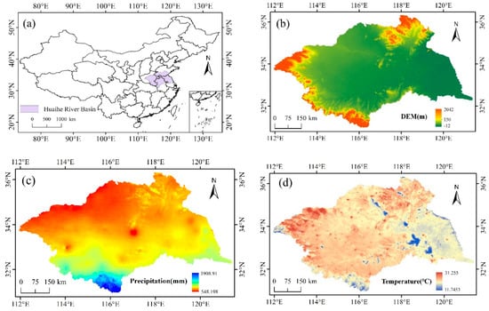
Figure 1.
(a) Geographical location of the Huai River Basin; (b) Digital elevation model (DEM); (c) Average precipitation from 1989 to 2017; (d) Average temperature from 1989 to 2017.
2.2. Data Source
2.2.1. Landsat5 TM, 7 ETM+, 8 OLI Data
The Huai River Basin covers 27 path/row of the Landsat Worldwide Reference System (WRS-2) (Figure 2c). The Landsat standard Level 1T (L1T) terrain-corrected orthorectified images, which are processed by the Landsat Ecosystem Interference Adaptive Processing System Algorithm (LEDAPS), are used in our study. Based on the GEE platform (https://earthengine.google.com/), all the Landsat (TM, ETM+, and OLI) surface seflectance images (16,760 scenes) were obtained from 1 January, 1989 to 31 December, 2017 (Figure 2). The distribution of Landsat images was shown in Figure 2, including the total observation numbers of per pixel (Figure 2a), good-quality observation numbers of per pixel (Figure 2b), the numbers of Landsat images in each path/row (Figure 2c), the total numbers of images from different sensors (Landsat 5/7/8) (Figure 2d), and the cumulative percentage of pixels with good observations of 0, 1, 2, 3, 4, [5,10), [10,20), [20,40), [40,80), [80,160), respectively during 1989–2017 (Figure 2e). The acquisition of high-quality satellite imagery is critical to generating an annual water map, so bad-quality satellite images caused by ineffective pixels, clouds, cloud shadows, and snow are masked using the Fmask. The spatial distribution of the number of annual good observations and total observations across the study area from 1984 to 2015 can be found in Supplementary Figures S1 and S2.
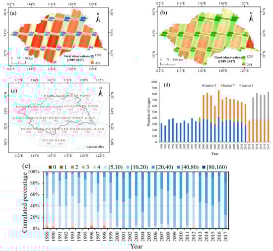
Figure 2.
The numbers distribution of Landsat 5, 7, 8 images in Huai River Basin from 1989 to 2017: (a) The total numbers of Landsat observation; (b) the total number of high-quality Landsat images; (c) the total number of Landsat images in each path/row (tiles); (d) the total number images of different Landsat sensors; (e) Cumulative percentage of pixels with good observations of 0, 1, 2, 3, 4, [5,10), [10,20), [20,40), [40,80), [80,160), respectively during 1989–2017.
2.2.2. Sentinel-2 Multispectral Instruments (MSI) Images, Globeland30, and Climate Data
Sentinel-2 is a European wide-scan, high-resolution, multi-spectral imaging sensor, which was successfully used to monitor vegetation, soil and water cover [45,46]. The Sentinel-2 MSI images were collected from 1 July, 2017 to 30 August, 2017 to closely match the period of the max surface water area to minimize bias that could arise because of large differences in time, and got the total number of 790 images in UTM/WGS84 projection to cover the study area. Sentinel-2 MSI data with the singular of 10 m was used to validate the accuracy of the Landsat extracted water map by visual interpretation. The Joint Research Centre Yearly Water Classification History (v1.0) dataset (JRC-data) [13] was also downloaded to compare with our results.
To validate our algorithm, this study firstly generated validation points from Globeland30, which can be downloaded from http://www.globallandcover.com/GLC30Download [11,47]. A systematic and random sampling method was adopted to select 1000 water surface points and 1000 non-water surface points from the water and non-water types of Globeland30, which are the water and non-water verification points evenly distribution across the Huai River Basin.
The annual average temperature, annual cumulative precipitation, and annual cumulative evapotranspiration is calculated from 3 h Global Land Data Assimilation System (GLDAS) product [48], which ingests satellite and ground-based observational data, and can be obtained based on the GEE platform.
2.3. Data Processing
2.3.1. Waterbody Area Extraction Algorithm
The modified normalized difference water index (mNDWI) is one of the most widely and efficiently used to delineate open water features using the green (band 2) and short-wave infrared (band 5) of Landsat TM, which can easily suppress the signal from built-up land noise [28]. However, mNDWI still has errors in distinguishing water bodies from vegetation [49,50]. Due to the mixed distributions of water and grasses in the wetlands, the wetland vegetation is the main factor leading to the classification errors of surface water bodies [51]. It has been suggested that combining mNDWI, the normalized water body index (NDVI) and enhanced vegetation index (EVI) can perform better and more stable than the individual index in delineating water [17,18,29,30,31]. Accordingly, this study used the combination of three indexes to extract surface water areas, which are EVI, NDVI, and mNDWI (Equations (1)–(3)). The criteria of mNDWI > NDVI and mNDWI > EVI were proved successfully to map surface water based on that water signal being stronger than the vegetation signal [17,18]. To reduce the interferences of wetland vegetation on the extraction of wetland water, the criteria of EVI < 0.1 can eliminate the interference of wetland vegetation. Therefore, the two criteria of (mNDWI > NDVI and EVI < 0.1) and (mNDWI > EVI and EVI < 0.1) were combined to identify the surface water bodies.
where ρred, ρgreen, ρblue, ρnir, and ρswir1 are the reflectance of the red band, green band, blue band, near-infrared band 1 and shortwave infrared band 1, respectively.
The detailed process consists of four major steps (Figure 3): Firstly, this study chose Landsat 5/7/8 surface reflectance Tier1 on the GEE platform across the Huai River Basin during 1989–2017, and performed masking on the collected images to remove the low-quality pixels caused by clouds, snow, and shadows using the function of Fmask. Secondly, EVI, NDVI, and mNDWI were calculated on a pixel-by-pixel basis, and extracted the surface water using the criteria of (mNDWI > NDVI and EVI < 0.1) or (mNDWI > EVI and EVI < 0.1). When the criteria were met, a pixel was classified as surface water which was then assigned to 1. On the contrary, the pixel was classified as non-water which was assigned to 0. Thirdly, the water body frequency was calculated, which is a ratio of the total number of water observations to the total number of good observations using all Landsat images within one year and multi-year. According to previous literature [17,18], when the annual water frequency was ≥0.25, the pixels were classified as an effective surface water, forming annual maximum water extent. When the annual water body frequency was ≥0.75, the pixels were classified as annual year-long water extents. When the annual water body frequency spanned from 0.25 to 0.75, the pixels were classified seasonal surface water areas. The annual average surface water area is the sum of all the effective water pixel’ s area (900 m2) multiplied by the water body frequency. Finally, this study calculated the annual area of the maximum, year-long, seasonal, and average surface water area from 1989 to 2017. The inter-annual variations and changing trends of surface water areas in the past 29 years were analyzed using a linear regression analysis.
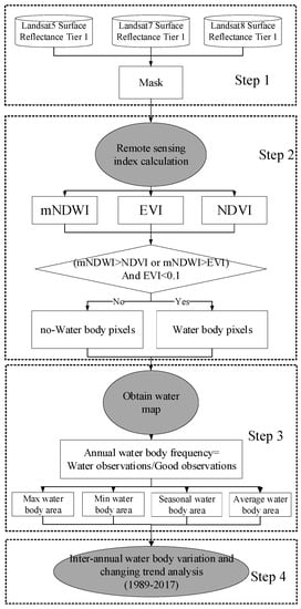
Figure 3.
A flowchart of the overall route of open surface water mapping using Landsat 5, 7, and 8 images and Google Earth Engine (GEE).
2.3.2. Variation Analysis
The precipitation, evapotranspiration, and temperature are used as the measures of regional climate and have direct relations with water body changes [52]. The trend of precipitation, evapotranspiration, temperature and four types of annual surface water area were analyzed using the Kendall-Theil regression, which is considered to be a robust linear trend regression method in previous studies [53,54]. To explore the relationship between the Huai River Basin water area and climatic factors, a linear correlation analysis was performed and tested for the four types of annual water area with the annual total precipitation, total evapotranspiration, and average temperature. c
2.4. Accuracy Assessment
Sentinel-2 MSI images with 10 m resolutions taken from 1 July, 2017 to 30 August, 2017 were used as the reference data. To maintain balanced sampling for the water and non-water zone, the 1000 points were stratified randomly selected in the water and non-water areas from the 30 m resolutions of the Globeland30 across the Huai River Basin, respectively. Then, 2000 points were added to the 10 m resolution Sentinel-2 MSI images and visually interpreted the water or non-water surfaces (Figure 4). The visually interpreted 2000 points served as reference data. Meanwhile, 2000 points were added to a single temporal surface water map, which was produced from 27 Landsat images from 1 July, 2017 to 30 August, 2017 in the Huai River Basin, to generate the confusion matrix with the producer’s (PA), the user’s (UA), the overall accuracies (OA) and the Kappa coefficient (Kc). The OA evaluated the overall performance of the model and is the proportion of correctly classified pixels and the sum of classified pixels. PA represents the agreement between the reference data and the classification, while UA evaluates how well the classified pixels agree with the known reference data. The UA and PA are related to commission and omission errors. The Kappa coefficient is the measure of the actual agreement between the reference data and the classifier used for the classification versus the chance of the agreement between the reference data and the random classifier. The Equation of PA, UA, OA, and Kc is as following:
where Stotal is the sum of correctly classified pixels, n is the sum of validation pixels, r is the number of rows, Sij is observation in a row i column j; Si is a marginal total of row i; Sj is a marginal total of column j.
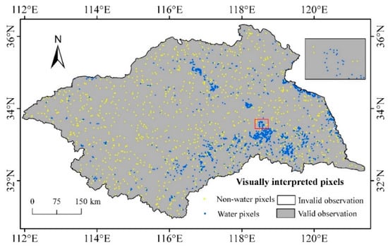
Figure 4.
Visually interpreted water and non-water pixels.
3. Results and Analysis
3.1. Accuracy Assessment of Single-Temporal Surface Water Map
As the maximum water areas, year-long water areas, and seasonally changing water areas were obtained from the same method and images, the classification accuracies of these maps are comparable. Therefore, this study just selected the maximum water areas as an example to validate the accuracies of our results. As shown in Table 1, each sampling point was visually interpreted as water or non-water pixels according to Sentinel-2 MSI images and a confusion matrix was generated. According to the confusion matrix, the overall accuracy of the water identification algorithm was 93.6%, the Kappa coefficient was 0.87, the producer’s accuracy was 89.64% and the user accuracy was 95.99%.

Table 1.
The confusion matrix and accuracy evaluation for the maximum surface water map of the Huai River Basin based on a visual inspection of Sentinel-2 MSI images.
3.2. Spatial Distribution of Surface Water in the Huai River Basin
There are approximately 11 million water pixels, in which the annual water frequency is larger than or equal to 0.25, in both the annual water frequency map of 2017 and the accumulated water frequency map of 1989–2017 across the Huai River Basin, accounting for 3.6% of the total area of the Huai River Basin (Figure 5a,b). The spatial distribution of water pixels at different frequencies in 2017 and 1989–2017 indicates that 52% and 47% of the water have a pixel frequency greater than 0.75 (Figure 5c,d). These water pixels consist of the interior of a large lake, a reservoir, and a river with water all year round. Due to the fluctuations of the water levels, the edge of a large water body may expose fully during the dry season water. For example, the water frequency map of the central area of Hongze Lake is close to 1, indicating that water is present all year round in the depth of the lake. The frequency level of the edge of the Hongze Lake is 0.63, indicating that the water is shallow and water disappears in some season. The pixel frequency value of the junction of the river and the lake (e.g., intersection of the Xuhong River and Hongze Lake) is less than 0.55, indicating that the water extent of the lake expands in a rainy season although the water is shallow. Small water bodies have lower pixel frequencies, indicating that they may only exist for a few months in a rainy season or become too small to be detected. The number of water pixels observed with 8 water frequency levels from 1989 to 2017 is shown in Figure 5e. The highest water frequency span 0.95 to 1, and the other water frequency levels are more or less.
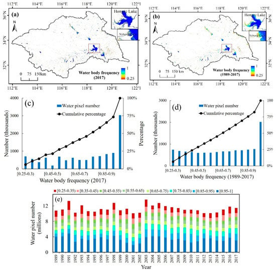
Figure 5.
The water frequency distribution in Huai River Basin: Water frequency distribution map of 2017 (a) and 1989–2017 (b); The number of pixel distributions of water at different frequency levels with a bin of 0.05 in 2017 (c) and 1984–2015 (d); The number of pixel distributions of water at different frequency levels with a bin of 0.1 during 1989–2017 (e).
Among the 11 million water pixels in 2017, there are 5.72 million water pixels of the year-long surface water body, which located in the central area of the lake, the reservoir, and the main river. The remaining 5.38 million water bodies are seasonal variations of water bodies, which are located in small ponds, tributaries, and lake edges. The maximum water area was 52% and the seasonal water area was 48%. According to the water frequency map of 1989–2017 (Figure 5b), large water bodies have higher water frequency, indicating that they have a higher probability of a continuous water surface throughout the year. In contrast, small bodies of water have lower water frequency, suggesting that they may be changed considerably by evaporation, recharge groundwater, less inflow caused by intensified irrigation, and less precipitation in some years, especially in related sectors such as public water, hydropower and animal husbandry.
3.3. Trends of Surface Water Area Variations in Huai River Basin from 1989 to 2017
The maximum, seasonal and average water body areas all showed a typical decreasing trend from 1989 to 2017, but the year-long water area showed a slight upward trend (Figure 6). The maximum water area varied from 9062 km2 to 12260 km2, which was 21% higher and 10.5% lower than the average area of 10130 km2, respectively. The year-long water area varied from 3465 km2 to 6650 km2, which was 35% below and 24% above the average value (5362 km2), respectively. The seasonal water area varied from 3698 km2 to 5742 km2 over seasons in one year, which was 22.3% below and 20.6% above the average value (4762 km2), respectively. Since the average water area is based on the pixel level of the water bodies, it can best reflect the changes in water bodies in one year. The average water area varied from 5878 km2 to 8794 km2, which was 19.4% below and 20.5% above the average value (7296 km2), respectively. As shown in Figure 6, the statistics of water bodies show a downward trend from 1989 to 2017, including the maximum water body area (p < 0.01), the seasonal water body area (p < 0.01), and the average water body area (p < 0.01). The water body with an upward trend found for the year-long water area (p < 0.01). In the past 29 years, the total surface water area of the Huai River Basin has generally shown a downward trend. According to the linear regression model, the average water area in the Huai River Basin decreased by 2.2 km2 per year in the past 29 years (Figure 6b).
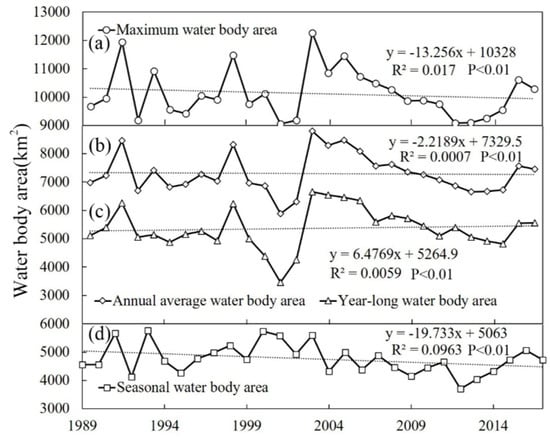
Figure 6.
The water area distribution in the Huai River Basin from 1989 to 2017: (a) The maximum water body; (b) the average water body; (c) the year-long water body; (d) seasonally changing water body.
The number of maximum and year-long water bodies showed similar patterns of decreasing tendency during 1989–2017 (Figure 7). The maximum number of water bodies varied from 200,000 to 320,000, which was 19% below and 29.5% above the average value (247,000), respectively. The year-long number of water bodies varied from 96,000 to 170,000, which was 26.1% below and 30.7% above the average value (130,000), respectively. The downward trend was found in the maximum number of water bodies (p < 0.01) and the year-long number of water bodies (p < 0.01). The downward trend in the number of water bodies indicates that some water bodies disappear year after year.
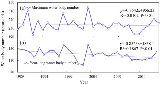
Figure 7.
The inter-annual variations of water body numbers across the Huai River Basin from 1989 to 2017: The numbers of maximum water body (a) and year-long water body (b).
The number and area distributions of maximum surface water bodies at different size levels are shown in Figure 8. In the maximum water body map, the water bodies are divided into 10 categories based on the size. From 1989 to 2017, water bodies which have area larger than 100 ha accounted for 0.23% of the total maximum water body numbers, and accounted for 75.9% of the total maximum water body area, 0.18% of the maximum water body number changes, and 74.5% of the total maximum water body area changes. However, the maximum water bodies which have area less than 0.5ha accounted for 80.6% of the maximum water body numbers, and accounted for 3% of the total maximum water body area, 84.6% of the maximum water body number changes, and 5.9% of the total maximum water body changes. Therefore, the number change of maximum water body in the Huai River Basin is mainly contributed by small water bodies, but the area change of the maximum water body is mainly contributed by large water bodies.
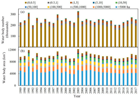
Figure 8.
The numbers and area distribution of the maximum surface water body at different size levels during 1989-2017; (a) the number distribution of maximum surface water, (b) the area distribution of maximum surface water.
3.4. Relationship Between the Climatic Factors and Huai River Basin’s Water
Figure 9 shows a consistent increase in evapotranspiration and temperature for the Huai River Basin. Meanwhile, an increasing trend in precipitation also has been observed. The evapotranspiration increases faster than precipitation, which aggravates aridification of the Huai River Basin.
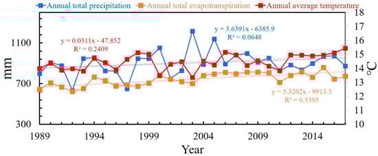
Figure 9.
Changes in annual total precipitation, total evapotranspiration, and the average temperature in the Huai River Basin during 1987–2017.
On the inter-annual scale, the precipitation in the Huai River Basin had a significant correlation with the Huai River maximum water body area (r = 0.6, p = 0.02) and average water body area (r = 0.56, p = 0.03) (Table 2). There is no significant correlation with the minimum water body area (p = 0.2) and the seasonal water body area (p > 0.05). The evapotranspiration and temperature also are not significantly (p > 0.05) correlated with the maximum, minimum, seasonal, and average water body area (Table 2). Therefore, precipitation in the Huai River Basin is the main climate factor which influences on the water body area.
Table 2.
Statistical summary of the linear correlation between the precipitation, evapotranspiration, temperature and the Huai River Basin’s water body area from 1989 to 2017.
3.5. Changes of Surface Water in Wet and Dry Years
Precipitation is one of the most important climate drivers for surface water changes [55], which has a strong impact on the total surface water area. The total annual rainfall of the Huai River Basin in 2001 and 2003 was 730 mm and 1203 mm, respectively (Figure 9). Compared with the average rainfall (914.5 mm) in the past 29 years, 2001 was a dry year while 2003 was a wet year. The maximum surface water map has more area and number of water bodies in the wet year of 2003 than in the dry year of 2001 (Figure 10a,b). In 2003, the number of water bodies was 320,000, which was 80,000 more than in 2001 (240,000). Among the two years difference of 80,000, the number of water bodies with an area less than 0.5 ha accounts for 80.9%, and the number of water bodies with an area spanning 0.5 ha to 5 ha accounts for 16.5%. Therefore, the changes in the total number of water bodies were mainly controlled by small water bodies, while small water bodies were more affected by precipitation. The water area increased by 3197.3 km2 from 2001 to 2003, water bodies with an area100 ha and above accounted for 71% of the additional water area in 2003, indicating that the change of surface water area was mainly affected by large surface water bodies.
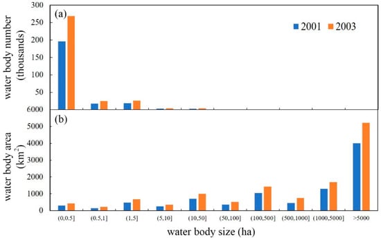
Figure 10.
The distribution and area distribution based on the water body range in 2001 and 2003: (a) The water body number distribution; (b) the water body size distribution.
4. Discussion
4.1. Comparison with JRC-Data
This study compared our identified surface waters with the JRC-data across the Huai River Basin (Figure 11). The JRC-data contains the global spatial and temporal distribution of surface water bodies from 1984 to 2015. The dataset was generated from Landsat 5, 7, and 8 images from March 16, 1984 to 10 October, 2015 with 3,066,102 scenes [13]. Each pixel was classified using an expert system to determine whether it was a water body. As the global scale is involved, surface water is only divided into seasonal surface water and permanent surface water by seasonal classification of water throughout the year. In order to comprehensively monitor the water variation, this study not only generated annual seasonal and permanent surface water, but also produced the annual maximum, and the average water body maps. At the same time, the details about the water body areas and numbers at different levels have been discussed. Finally, the maximum surface water (the sum of seasonal and permanent surface water) and seasonal surface water were produced by JRC-data. This study selected five different water types (lakes (a), rivers (b), ponds (c), mountain waters (d) and urban water bodies (e)) to quantify the similarity and difference between the annual surface water map in this study and the JRC-data. Figure 11 shows that the surface water profiles identified and drawn in two ways are comparable. The JRC-data defines seasonal surface water and permanent surface water by the appearance of monthly surface water obtained by image-wise processing with digital elevation models, glacier data, urban areas data, and lava mask, resulting in a comprehensive result. However, our study using the algorithm of remote sensing vegetation index combined with a water body index to identify and map surface water bodies is much simpler.
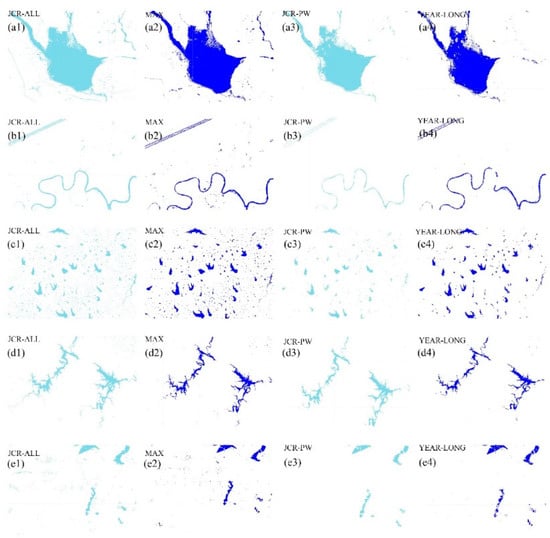
Figure 11.
A comparison between the water map generated in this study (MAX (a2–e2) denotes the maximum water body, and YEAR-LONG (a4–e4) denotes the year-long water body) and JRC-data (JRC-All represents the sum of the annual seasonal surface water and permanent surface water (a1–e1), and JRC-PW represents permanent surface water of the JRC-data (a3–e3). Lakes (a), rivers (b), ponds (c), mountain waters (d) and urban water bodies (e).
4.2. Impacts of Climate Change and Human Activities on the Temporal and Spatial Patterns of Surface Water Bodies
Precipitation is the main source of water in the Huai River Basin, and an increase in rainfall usually leads to an increase in the water area. The temperature and evapotranspiration had no significant negative effect on the annual average water area and the annual continuous water area, even though the high temperature increases evaporation through enhancing vapor pressure deficit. The high temperature also increases the demand for agricultural irrigation, which leads to water withdrawal and then decreasing the surface water area [31].
According to the 2016 Huai River Water Resources Bulletin, the surface water in the Huai River Basin is mainly used for farmland irrigation, industrial, domestic water and forestry, animal husbandry and fishery, which accounts for 63.4%, 14.1%, 10.4% and 7.2% of the total water consumption, respectively. In terms of human activities, the population and GDP of the Huai River Basin have grown rapidly in recent decades, particularly in the 2000s [56]. With industrialization and urbanization, some surface water bodies have become construction areas. By analyzing the trend of the maximum, seasonal and average surface water distribution in the Huai River Basin from 1989 to 2017, this study found that they all show a weak downward trend. As shown in Figure 5, since 2003, the change of surface water areas in the Huai River Basin has tended to be moderate. This is mainly due to the increasing emphasis on environmental protection and water resources protection by the central and local governments, especially for the protection of lakes and reservoirs. Furthermore, 216 large and medium-sized reservoirs in the Huai River Basin, such as lakes and Linhuaigang, have played an important role in maintaining the relative stability of surface water.
Due to the changes in precipitation intensity and frequency, the Huai River Basin would have a higher frequency and more severe drought [57]. Therefore, the surface water area is more likely to decrease, and it is likely to refresh its minimum record in the future. The problems bring challenges to the sustainable economic and social development of the Huai River Basin and the stability of the ecosystem. In addition to climate drivers, agricultural irrigation, water wastage, mining and water conservancy projects can lead to changes in water bodies.
4.3. Uncertainties of this Study
The Huai River Basin has a large number of small ponds and lakes, and these small water bodies tend to have larger areas during the wet seasons. In order to represent the intra- and inter-annual changes in water bodies, this study adopted four water-related indices (the maximum water area, the year-long water area, the average water area, and the seasonal water area), using the algorithms based on the combination of NDVI, EVI, and mNDWI, rather than single index and specific thresholds. Selecting a specific threshold may have subjective factors and be time-consuming [50], and the selected threshold applied to different images and times in different regions can introduce unpredictable uncertainties [49]. In addition, the method used in this study cannot detect water beneath a closed canopy.
The errors in the classification in this study are mainly caused by omission errors, and the missing errors are superior to commission errors in most water indices [58,59,60]. The mixed pixels at the edge of the water bodies are the main cause of missing water pixels [58], including narrow rivers often without any or only partial observations due to their weak water signals in mixed pixels [9]. The main water bodies in the Huai River Basin are usually wide, and water and sedimentary rivers occupy part of the riverbed, so many of the rivers in this study appear in seasonal water maps rather than annual persistent water maps. Asphalt roads, mountain shadows, and buildings all have low surface reflectance, which is the main cause of redundancy classification in water classification [50,61,62]. Although pixels contaminated by cloud have been excluded in the data preprocessing, residual clouds and shadows still affect the classification accuracies.
5. Conclusions
This study adopted an integrated approach by combining the vegetation index and the water index to quantify the spatiotemporal variability of surface water bodies in the Huai River Basin during 1989–2017 from muti-temporal Landsat TM, ETM+ and OLI imagery based on GEE. The results demonstrate that our adopted method is effective to monitor the temporal and spatial variations of surface water bodies at a spatial resolution of 30 m. The maximum, average and seasonal variations of surface water areas in the Huai River Basin showed a downward trend in the past 29 years, while the year-long surface water area showed a slight upward trend. The surface water area was positively correlated with precipitation (p < 0.05) and negatively correlated with temperature and evapotranspiration (p > 0.05), and the small water bodies had the highest probability to disappear under drought conditions. The area and number of the surface water bodies in the Huai River Basin showed a downward trend in the past 29 years, and the changes of numbers of water bodies mainly depended on the number of small surface water bodies, and the changes of total surface water area were mainly controlled by larger surface water bodies. Our results provide important references for water-management policies and shifts in agricultural production in the context of continuous climate warming.
Supplementary Materials
The following are available online at https://www.mdpi.com/2072-4292/11/15/1824/s1. Figure S1: Total numbers of Landsat total observation for pixel-by-pixel from 1989 to 2017. Figure S2: Total numbers of Landsat good observation for pixel-by-pixel from 1989 to 2017. Figure S3: Water body frequency threshold selection, The first line is maximum water body area using 14 different water body frequency thresholds, The second line is noise conditions of insets in the 2017 maximum water body maps using threshold:0.1,0.15,0.2,0.25. Figure S4: Water detection in built-up and vegetation land. (a) Landsat 8 OLI surface reflectance image (list bands in the false-color composite (bands 5,4,3)), (b) Final water detection in blue color ((mNDWI>NDVI or mNDWI>EVI) and (EVI<0.1)), (c) EVI, (d) Scatter plot ((mNDWI-NDVI) vs EVI), (e) Scatter plot ((mNDWI-NDVI) vs EVI) with water detection marked red, (f) Surface water in red corresponding to water detection in scatter plot e, (g) Scatter plot ((mNDWI-EVI) vs EVI), (h) Scatter plot ((mNDWI-EVI) vs EVI) with water detection marked red, (i) Surface water in red corresponding to water detection in scatter plot h.
Author Contributions
H.X. and Y.Q. conceived and designed the experiments. H.X. and J.Z. performed the programming work, analysis, discussions, and wrote most sections of the manuscript. H.X., Y.Q., J.Y., Y.C., H.S., L.M., N.J. and Q.M. supplied suggestions and comments and revised the manuscript. All authors reviewed and adjusted the manuscript.
Funding
This research was funded jointly by the National Natural Science Foundation Project of China (41601091, 41701186, 41701503, and 41701433), the Program for Key Scientific Research in the University of Henan Province (18A170002), the Open Fund of CMA·Henan Key Laboratory of Agrometeorological Support and Applied Technique(AMF201809), and the National Key Research and Development Program of China (2016YFA0600103, 2016YFC0500201-06). We are grateful to all contractors, image providers, and the anonymous reviewers for their valuable comments and suggestions.
Acknowledgments
All authors thank the anonymous reviewers and the editor for the constructive comments on the earlier version of the manuscript.
Conflicts of Interest
The authors declare no conflicts of interest.
References
- Amprako, J.L. The United Nations World Water Development Report 2015: Water for a Sustainable World. Future Food J. Food Agric. Soc. 2016, 4, 64–65. [Google Scholar]
- Hall, J.W.; Grey, D.; Garrick, D.; Fung, F.; Brown, C.; Dadson, S.J.; Sadoff, C.W. Coping with the curse of freshwater variability. Science 2014, 346, 429–430. [Google Scholar] [CrossRef] [PubMed]
- Tulbure, M.G.; Broich, M.; Stehman, S.V.; Kommareddy, A. Surface water extent dynamics from three decades of seasonally continuous Landsat time series at subcontinental scale in a semi-arid region. Remote Sens. Environ. 2016, 178, 142–157. [Google Scholar] [CrossRef]
- Shilong, P.; Philippe, C.; Yao, H.; Zehao, S.; Shushi, P.; Junsheng, L.; Liping, Z.; Hongyan, L.; Yuecun, M.; Yihui, D.; et al. The impacts of climate change on water resources and agriculture in China. Nature 2010, 467, 43–51. [Google Scholar]
- Qi, H.; Altinakar, M.S. Simulation-based decision support system for flood damage assessment under uncertainty using remote sensing and census block information. Nat. Hazards 2011, 59, 1125–1143. [Google Scholar] [CrossRef]
- Zhang, J.; Zhou, C.; Xu, K.; Watanabe, M. Flood disaster monitoring and evaluation in China. Glob. Environ. Chang. Part B Environ. Hazards 2002, 4, 33–43. [Google Scholar] [CrossRef]
- Barton, I.J.; Bathols, J.M. Monitoring floods with AVHRR. Remote Sens. Environ. 1989, 30, 89–94. [Google Scholar] [CrossRef]
- Carroll, M.; Wooten, M.; DiMiceli, C.; Sohlberg, R.; Kelly, M. Quantifying Surface Water Dynamics at 30 Meter Spatial Resolution in the North American High Northern Latitudes 1991–2011. Remote Sens. 2016, 8. [Google Scholar] [CrossRef]
- Feng, M.; Sexton, J.O.; Channan, S.; Townshend, J.R. A global, high-resolution (30-m) inland water body dataset for 2000: First results of a topographic-spectral classification algorithm. Int. J. Digit. Earth 2016, 9, 113–133. [Google Scholar] [CrossRef]
- Li, S.; Sun, D.; Goldberg, M.; Stefanidis, A. Derivation of 30-m-resolution water maps from TERRA/MODIS and SRTM. Remote Sens. Environ. 2013, 134, 417–430. [Google Scholar] [CrossRef]
- Liao, A.; Chen, L.; Chen, J.; He, C.; Cao, X.; Chen, J.; Peng, S.; Sun, F.; Gong, P. High-resolution remote sensing mapping of global land water. Sci. China Earth Sci. 2014, 57, 2305–2316. [Google Scholar] [CrossRef]
- Mueller, N.; Lewis, A.; Roberts, D.; Ring, S.; Melrose, R.; Sixsmith, J.; Lymburner, L.; Mcintyre, A.; Tan, P.; Curnow, S.; et al. Water observations from space: Mapping surface water from 25 years of Landsat imagery across Australia. Remote Sens. Environ. 2016, 174, 341–352. [Google Scholar] [CrossRef]
- Pekel, J.F.; Cottam, A.; Gorelick, N.; Belward, A.S. High-resolution mapping of global surface water and its long-term changes. Nature 2016, 540, 418–422. [Google Scholar] [CrossRef] [PubMed]
- Sheng, Y.; Song, C.; Wang, J.; Lyons, E.A.; Knox, B.R.; Cox, J.S.; Feng, G. Representative lake water extent mapping at continental scales using multi-temporal Landsat-8 imagery. Remote Sens. Environ. 2016, 185, 129–141. [Google Scholar] [CrossRef]
- Xia, H.; Zhao, W.; Li, A.; Bian, J.; Zhang, Z. Subpixel Inundation Mapping Using Landsat-8 OLI and UAV Data for a Wetland Region on the Zoige Plateau, China. Remote Sens. 2017, 9. [Google Scholar] [CrossRef]
- Dai, Y.; Trigg, M.A.; Ikeshima, D. Development of a global—90 m water body map using multi-temporal Landsat images. Remote Sens. Environ. 2015, 171, 337–351. [Google Scholar]
- Zou, Z.; Dong, J.; Menarguez, M.A.; Xiao, X.; Hambright, K.D. Continued decrease of open surface water body area in Oklahoma during 1984–2015. Sci. Total Environ. 2017, 595, 451–460. [Google Scholar] [CrossRef]
- Zou, Z.; Xiao, X.; Dong, J.; Qin, Y.; Doughty, R.B.; Menarguez, M.A.; Zhang, G.; Wang, J. Divergent trends of open-surface water body area in the contiguous United States from 1984 to 2016. Proc. Natl. Acad. Sci. USA 2018, 115, 3810–3815. [Google Scholar] [CrossRef]
- Li, W.; Du, Z.; Ling, F.; Zhou, D.; Wang, H.; Gui, Y.; Sun, B.; Zhang, X. A Comparison of Land Surface Water Mapping Using the Normalized Difference Water Index from TM, ETM plus and ALI. Remote Sens. 2013, 5, 5530–5549. [Google Scholar] [CrossRef]
- Roberts, D.A.; Gardner, M.; Church, R.; Ustin, S.; Scheer, G.; Green, R.O. Mapping Chaparral in the Santa Monica Mountains Using Multiple Endmember Spectral Mixture Models. Remote Sens. Environ. 1998, 65, 267–279. [Google Scholar] [CrossRef]
- Smith, M.; Adams, J.; Gillespie, A. Reference endmembers for spectral mixture analysis. In Proceedings of the 5th Australasian Remote Sensing Conference, Perth, Australia, 8–12 October 1990; pp. 331–340. [Google Scholar]
- Henits, L.; Jürgens, C.; Mucsi, L. Seasonal multitemporal land-cover classification and change detection analysis of Bochum, Germany, using multitemporal Landsat TM data. Int. J. Remote Sens. 2016, 37, 16. [Google Scholar] [CrossRef]
- Evora, N.D.; Tapsoba, D.; De Seve, D. Combining artificial neural network models, geostatistics, and passive microwave data for snow water equivalent retrieval and mapping. IEEE Trans. Geosci. Remote Sens. 2008, 46, 1925–1939. [Google Scholar] [CrossRef]
- Li, E.; Du, P.; Samat, A.; Xia, J.; Che, M. An automatic approach for urban land-cover classification from Landsat-8 OLI data. Int. J. Remote Sens. 2015, 36, 5983–6007. [Google Scholar] [CrossRef]
- Rundquist, D.C.; Lawson, M.P.; Queen, L.P.; Cerveny, R.S. The Relationship between Summer-Season Rainfall Events and Lake-Surface Area1. JAWRA J. Am. Water Resour. Assoc. 1987, 23, 493–508. [Google Scholar] [CrossRef]
- Gao, B.C. NDWI—A normalized difference water index for remote sensing of vegetation liquid water from space. Remote Sens. Environ. 1996, 58, 257–266. [Google Scholar] [CrossRef]
- Mcfeeters, S.K. The use of the Normalized Difference Water Index (NDWI) in the delineation of open water features. Int. J. Remote Sens. 1996, 17, 1425–1432. [Google Scholar] [CrossRef]
- Xu, H. Modification of normalised difference water index (NDWI) to enhance open water features in remotely sensed imagery. Int. J. Remote Sens. 2006, 27, 3025–3033. [Google Scholar] [CrossRef]
- Chen, B.; Xiao, X.; Li, X.; Pan, L.; Doughty, R.; Ma, J.; Dong, J.; Qin, Y.; Zhao, B.; Wu, Z.; et al. A mangrove forest map of China in 2015: Analysis of time series Landsat 7/8 and Sentinel-1A imagery in Google Earth Engine cloud computing platform. ISPRS J. Photogramm. Remote Sens. 2017, 131, 104–120. [Google Scholar] [CrossRef]
- Dong, J.; Xiao, X.; Menarguez, M.A.; Zhang, G.; Qin, Y.; Thau, D.; Biradar, C.; Moore, B., III. Mapping paddy rice planting area in northeastern Asia with Landsat 8 images, phenology-based algorithm and Google Earth Engine. Remote Sens. Environ. 2016, 185, 142–154. [Google Scholar] [CrossRef]
- Wang, X.; Xiao, X.; Zou, Z.; Chen, B.; Ma, J.; Dong, J.; Doughty, R.B.; Zhong, Q.; Qin, Y.; Dai, S.; et al. Tracking annual changes of coastal tidal flats in China during 1986–2016 through analyses of Landsat images with Google Earth Engine. Remote Sens. Environ. 2018, 110987. [Google Scholar] [CrossRef]
- Feng, L.; Hu, C.; Chen, X.; Li, R. Satellite observations make it possible to estimate Poyang Lake's water budget. Environ. Res. Lett. 2011, 6. [Google Scholar] [CrossRef]
- Homer, C.; Dewitz, J.; Yang, L.; Jin, S.; Danielson, P.; Xian, G.; Coulston, J.; Herold, N.; Wickham, J.; Megown, K. Completion of the 2011 National Land Cover Database for the Conterminous United States—Representing a Decade of Land Cover Change Information. Photogramm. Eng. Remote Sens. 2015, 81, 345–354. [Google Scholar] [CrossRef]
- Liu, H.; Yin, Y.; Piao, S.; Zhao, F.; Engels, M.; Ciais, P. Disappearing Lakes in Semiarid Northern China: Drivers and Environmental Impact. Environ. Sci. Technol. 2013, 47, 12107–12114. [Google Scholar] [CrossRef]
- Wulder, M.A.; Loveland, T.R.; Roy, D.P.; Crawford, C.J.; Masek, J.G.; Woodcock, C.E.; Allen, R.G.; Anderson, M.C.; Belward, A.S.; Cohen, W.B.; et al. Current status of Landsat program, science, and applications. Remote Sens. Environ. 2019, 225, 127–147. [Google Scholar] [CrossRef]
- Zhu, Z.; Wulder, M.A.; Roy, D.P.; Woodcock, C.E.; Hansen, M.C.; Radeloff, V.C.; Healey, S.P.; Schaaf, C.; Hostert, P.; Strobl, P.; et al. Benefits of the free and open Landsat data policy. Remote Sens. Environ. 2019, 224, 382–385. [Google Scholar] [CrossRef]
- Gorelick, N.; Hancher, M.; Dixon, M.; Ilyushchenko, S.; Thau, D.; Moore, R. Google Earth Engine: Planetary-scale geospatial analysis for everyone. Remote Sens. Environ. 2017, 202, 18–27. [Google Scholar] [CrossRef]
- Huang, H.; Chen, Y.; Clinton, N.; Jie, W.; Wang, X.; Liu, C.; Peng, G.; Yang, J.; Bai, Y.; Zheng, Y.; et al. Mapping major land cover dynamics in Beijing using all Landsat images in Google Earth Engine. Remote Sens. Environ. 2017, 202, 166–176. [Google Scholar] [CrossRef]
- Liu, X.; Hu, G.; Chen, Y.; Li, X.; Xu, X.; Li, S.; Pei, F.; Wang, S. High-resolution multi-temporal mapping of global urban land using Landsat images based on the Google Earth Engine Platform. Remote Sens. Environ. 2018, 209, 227–239. [Google Scholar] [CrossRef]
- Chen, B.; Xiao, X.; Ye, H.; Ma, J.; Doughty, R.; Li, X.; Zhao, B.; Wu, Z.; Sun, R.; Dong, J.; et al. Mapping Forest and Their Spatial-Temporal Changes From 2007 to 2015 in Tropical Hainan Island by Integrating ALOS/ALOS-2 L-Band SAR and Landsat Optical Images. IEEE J. Sel. Top. Appl. Earth Obs. Remote Sens. 2018, 11, 852–867. [Google Scholar] [CrossRef]
- Xiong, J.; Thenkabail, P.S.; Tilton, J.C.; Gumma, M.K.; Teluguntla, P.; Oliphant, A.; Congalton, R.G.; Yadav, K.; Gorelick, N. Nominal 30-m Cropland Extent Map of Continental Africa by Integrating Pixel-Based and Object-Based Algorithms Using Sentinel-2 and Landsat-8 Data on Google Earth Engine. Remote Sens. 2017, 9. [Google Scholar] [CrossRef]
- Wang, C.; Jia, M.; Chen, N.; Wang, W. Long-Term Surface Water Dynamics Analysis Based on Landsat Imagery and the Google Earth Engine Platform: A Case Study in the Middle Yangtze River Basin. Remote Sens. 2018, 10, 1635. [Google Scholar] [CrossRef]
- Gao, C.; Chen, S.; Zhai, J.; Zhang, Z.; Liu, Q. On threshold of drought and flood disasters in Huaihe River basin. Adv. Water Sci. 2014, 25, 36–44. [Google Scholar]
- Gao, C.; Zhang, Z.; Zhai, J.; Qing, L.; Yao, M. Research on meteorological thresholds of drought and flood disaster: A case study in the Huai River Basin, China. Stoch. Environ. Res. Risk Assess. 2015, 29, 157–167. [Google Scholar] [CrossRef]
- Yang, X.; Zhao, S.; Qin, X.; Na, Z.; Liang, L. Mapping of Urban Surface Water Bodies from Sentinel-2 MSI Imagery at 10 m Resolution via NDWI-Based Image Sharpening. Remote Sens. 2017, 9, 596. [Google Scholar] [CrossRef]
- Gong, P.; Liu, H.; Zhang, M.; Li, C.; Wang, J.; Huang, H.; Clinton, N.; Ji, L.; Li, W.; Bai, Y.; et al. Stable classification with limited sample: Transferring a 30-m resolution sample set collected in 2015 to mapping 10-m resolution global land cover in 2017. Sci. Bull. 2019, 64, 370–373. [Google Scholar] [CrossRef]
- Chen, J.; Ban, Y.; Li, S. China: Open access to Earth land-cover map. Nature 2014, 514, 434. [Google Scholar]
- Rodell, M.; Houser, P.; Jambor, U.; Gottschalck, J.; Mitchell, K.; Meng, C.J.; Arsenault, K.; Cosgrove, B.; Radakovich, J.; Bosilovich, M.; et al. The global land data assimilation system. Bull. Am. Meteorol. Soc. 2004, 85, 381–394. [Google Scholar] [CrossRef]
- Lei, J.I.; Zhang, L.I.; Wylie, B. Analysis of Dynamic Thresholds for the Normalized Difference Water Index. Photogramm. Eng. Remote Sens. 2009, 75, 1307–1317. [Google Scholar]
- Verpoorter, C.; Kutser, T.; Tranvik, L. Automated Mapping of Water Bodies Using Landsat Multispectral Data. Limnol. Oceanogr. Methods 2015, 10, 1037–1050. [Google Scholar] [CrossRef]
- Santoro, M.; Wegmueller, U.; Lamarche, C.; Bontemps, S.; Defoumy, P.; Arino, O. Strengths and weaknesses of multi-year Envisat ASAR backscatter measurements to map permanent open water bodies at global scale. Remote Sens. Environ. 2015, 171, 185–201. [Google Scholar] [CrossRef]
- Tao, S.; Fang, J.; Zhao, X.; Zhao, S.; Shen, H.; Hu, H.; Tang, Z.; Wang, Z.; Guo, Q. Rapid loss of lakes on the Mongolian Plateau. Proc. Natl. Acad. Sci. USA 2015, 112, 2281–2286. [Google Scholar] [CrossRef]
- Wang, Y.; Ma, J.; Xiao, X.; Wang, X.; Dai, S.; Zhao, B. Long-Term Dynamic of Poyang Lake Surface Water: A Mapping Work Based on the Google Earth Engine Cloud Platform. Remote Sens. 2019, 11, 313. [Google Scholar] [CrossRef]
- Theil, H. A rank-invariant method of linear and polynomial regression analysis. In Henri Theil’s Contributions to Economics and Econometrics; Springer: Berlin/Heidelberg, Germany, 1992; pp. 345–381. [Google Scholar]
- Bates, B.; Kundzewicz, Z.W.; Wu, S.; Palutikof, J. Climate Change and Water: Technical Paper VI. Environ. Policy Collect. 2008, 128, 343–355. [Google Scholar]
- Gao, C.; Ruan, T. The influence of climate change and human activities on runoff in the middle reaches of the Huaihe River Basin, China. J. Geogr. Sci. 2018, 28, 79–92. [Google Scholar] [CrossRef]
- Mo, X.; Hu, S.; Lu, H.; Lin, Z.; Liu, S. Drought Trends over the Terrestrial China in the 21st Century in Climate Change Scenarios with Ensemble GCM Projections. J. Nat. Resour. 2018, 33, 1244–1256. [Google Scholar]
- Feyisa, G.L.; Meilby, H.; Fensholt, R.; Proud, S.R. Automated Water Extraction Index: A new technique for surface water mapping using Landsat imagery. Remote Sens. Environ. 2014, 140, 23–35. [Google Scholar] [CrossRef]
- Fisher, A.; Flood, N.; Danaher, T. Comparing Landsat water index methods for automated water classification in eastern Australia. Remote Sens. Environ. 2016, 175, 167–182. [Google Scholar] [CrossRef]
- Rokni, K.; Musa, T.A.; Hazini, S.; Ahmad, A.; Solaimani, K. Investigating the application of pixel-level and product-level image fusion approaches for monitoring surface water changes. Nat. Hazards 2015, 78, 219–230. [Google Scholar] [CrossRef]
- Jakimow, B.; Griffiths, P.; Linden, S.V.D.; Hostert, P. Mapping pasture management in the Brazilian Amazon from dense Landsat time series. Remote Sens. Environ. 2017, 205, 453–468. [Google Scholar] [CrossRef]
- Tang, Z.; Ou, W.; Yue, D.; Yu, X. Extraction of Water Body Based on LandSat TM5 Imagery—A Case Study in the Yangtze River. IFIP Adv. Inf. Commun. Technol. 2012, 393, 416–420. [Google Scholar]
© 2019 by the authors. Licensee MDPI, Basel, Switzerland. This article is an open access article distributed under the terms and conditions of the Creative Commons Attribution (CC BY) license (http://creativecommons.org/licenses/by/4.0/).