Long-Term Spatial and Temporal Monitoring of Cyanobacteria Blooms Using MODIS on Google Earth Engine: A Case Study in Taihu Lake

Abstract

As cyanobacteria blooms occur in many types of inland water, routine monitoring that is fast and accurate is important for environment and drinking water protection. Compared to field investigations, satellite remote sensing is an efficient and effective method for monitoring cyanobacteria blooms. However, conventional remote sensing monitoring methods are labor intensive and time consuming, especially when processing long-term images. In this study, we embedded related processing procedures in Google Earth Engine, developed an operational cyanobacteria bloom monitoring workflow. Using this workflow, we measured the spatiotemporal patterns of cyanobacteria blooms in China’s Taihu Lake from 2000 to 2018. The results show that cyanobacteria bloom patterns in Taihu Lake have significant spatial and temporal differentiation: the interannual coverage of cyanobacteria blooms had two peaks, and the condition was moderate before 2006, peaked in 2007, declined rapidly after 2008, remained moderate and stable until 2015, and then reached another peak around 2017; bays and northwest lake areas had heavier cyanobacteria blooms than open lake areas; most cyanobacteria blooms primarily occurred in April, worsened in July and August, then improved after October. Our analysis of the relationship between cyanobacteria bloom characteristics and environmental driving factors indicates that: from both monthly and interannual perspectives, meteorological factors are positively correlated with cyanobacteria bloom characteristics, but as for nutrient loadings, they are only positively correlated with cyanobacteria bloom characteristics from an interannual perspective. We believe reducing total phosphorous, together with restoring macrophyte ecosystem, would be the necessary long-term management strategies for Taihu Lake. Our workflow provides an automatic and rapid approach for the long-term monitoring of cyanobacteria blooms, which can improve the automation and efficiency of routine environmental management of Taihu Lake and may be applied to other similar inland waters.

1. Introduction

Under the background of accelerated industrialization and urbanization, harmful algae blooms (HABs) occur frequently in inland and coastal waters due to eutrophication, which is the combined result of natural and anthropogenic processes, although it is primarily caused by inputs of anthropogenic nutrient loadings (nitrogen and phosphorus) [1]. Some species of algae blooms, such as cyanobacteria, can release odors and toxic compounds that are harmful to aquatic creatures and water ecosystems [1,2,3]. Cyanobacteria blooms propagate as a result of many environmental factors, such as temperature, precipitation, wind speed, atmospheric pressure, solar radiation, and nutrient loadings (nitrogen and phosphorus) [1,3,4,5,6,7,8,9]. Generally, those environmental driving variables are divided into two types: meteorological variables and water quality variables. Determining the relationship between cyanobacteria blooms and environmental driving factors is important for precaution and management.

Different methods have been used to model the formation and dynamics of cyanobacteria blooms. Some cyanobacteria bloom characteristics, together with their meteorological and water quality factors, are the main predictive variables in these models [10,11,12]. Artificial salvage of floating cyanobacteria also heavily relies on its location being determined in advance. Therefore, accurate and efficient monitoring of the spatiotemporal distributions of cyanobacteria blooms is vital for prevention and management. Field investigations by ship surveys and laboratory measurements are the basis of the conventional monitoring approach [13], but these methods can destroy the vertical and horizontal distributions of floating cyanobacteria, and are only able to detect the cyanobacteria biomass concentration along routes, therefore, the representativeness of limited water samples cannot be guaranteed. Field investigations cannot explain the spatial distribution of cyanobacteria blooms, and are expensive and labor-intensive [2,14,15]. Due to the large spatial coverage and short revisit interval of some satellite sensors, optical remote sensing could be used to effectively and efficiently monitor cyanobacteria blooms.

Many studies have monitored cyanobacteria blooms over inland and coastal waters. Reflectance classification [14], single-band threshold [5], water color indices [15,16,17,18], and bio-optical models [4] have been developed in water component remote sensing inversions. Among the many water color indices, the floating algae index (FAI) is an effective spectrum index for distinguishing floating cyanobacteria [16]. It has already been used for cyanobacteria bloom extraction in China’s Taihu Lake [15]. Unlike the normalized difference vegetation index (NDVI) and the enhanced vegetation index (EVI), the baseline subtraction method used by FAI can effectively remove cloud, sunglint, and geometry contamination, and is more stable for extracting long-term series of cyanobacteria blooms [15,16,19,20]. Since its development in 2010 [16], several studies have used FAI as a detector to extract long-term spatiotemporal patterns of blooms corresponding to cyanobacteria or other phytoplankton species. Hu et al. developed a workflow for extracting cyanobacteria bloom events in Taihu Lake and reconstructed its spatiotemporal patterns between 2000 and 2008 [15]. Hu et al. retrieved Ulva prolifera bloom dynamics from the Yellow Sea and East China Sea from 2000 to 2009 [21]. Huang et al. determined variations in cyanobacteria blooms from 2000 to 2011 in Taihu Lake [22]. Zhang et al. extracted the subpixel-level floating algae spatiotemporal dynamics in China’s Chaohu Lake over a period of 2000–2013 [23]. Kabenge et al. reconstructed floating algae patterns in Uganda’s Murchison Bay between 1990 and 2014 [24]. Zhang et al. determined the spatiotemporal bloom patterns in Taihu Lake from 2001 to 2013 [6]. Wang and Hu determined the distribution and coverage area of Sargassum from over the Central West Atlantic region during 2000–2015 [25]. Shi et al. identified the monthly and interannual cyanobacteria bloom temporal variations in Taihu Lake from 2003 to 2013 [26].

All the above listed studies used moderate resolution imaging spectroradiometer (MODIS) level 0 data, and the raw data were calibrated by SeaDAS software (NASA, US), in order to obtain the Rayleigh-corrected reflectance data for extracting floating cyanobacteria. For general end users, calibrating the huge amount of MODIS level 0 data required for specific applications is difficult. Other conventional remote sensing procedures for cyanobacteria blooms, including satellite image downloading, preprocessing, and spatial analysis, are also labor intensive and time consuming. These shortcomings have hindered the further extension of automatic remote sensing monitoring of long-term cyanobacteria blooms.

In some environmental monitoring scenarios that require large-scale satellite remote sensing data processing, thematic cloud-based platforms may perform better. The Google Earth Engine (GEE) is a cloud platform for geospatial data analysis, and has changed the traditional mode of processing used remote sensing [27]. GEE is especially suitable for long-term and large-scale spatiotemporal series of remote sensing applications; its multi-petabyte geospatial data and high-performance computation capacity provide a new approach to understanding the earth. Conventional remote sensing algorithms and methods, which were initially conducted with small-scale data, have the potential to be embedded and integrated in GEE, and applied in a variety of fields and scenarios. In the Web of Science database, we analyzed nearly 200 articles that have used GEE; most of their themes were roughly related to agriculture applications or urban or forest mapping. Overall, land use and land cover classification was the most common and prevailing topic. However, optical constituent studies of inland and coastal waters are rare [28,29,30,31,32], due largely to the complexity of bio-optical properties of case II water [3,4,15]. What is more, the lack of embedded water-leaving reflectance products of GEE has hindered the further operational applications in case II water. It is necessary to find and develop available operational inland water processing algorithms and perform them on GEE’s existing embedded datasets.

Based on the urgent need for long-term assessment of cyanobacteria blooms in eutrophic inland water, and recent developments in cloud-based technology, the objectives of our study were to (1) develop an operational workflow in GEE to accomplish rapid and automatic monitoring of long-term cyanobacteria blooms, (2) analyze the spatiotemporal patterns of cyanobacteria blooms in Taihu Lake over the most recent 19 years (2000 to 2018), and (3) determine the relationship between cyanobacteria blooms and environmental driving factors using our study’s monitoring data.

2. Materials and Methods

2.1. Study Area

Taihu Lake, the third largest freshwater lake in China, is located in the prosperous Yangtze River Delta (Figure 1). Its water surface coverage is approximately 2338 km², and it has a shallow mean water depth of 1.9 m [2,5,15]. It is a typical subtropical lake and is influenced by monsoons. Taihu Lake is one of the most important sources of drinking water for adjacent cities, such as Wuxi city [2,5]. Due to eutrophication lasting for more than two decades [8], cyanobacteria blooms frequently occur in Taihu Lake [33], and they have had negative effects on aquatic life and human health [34]. The cyanobacteria blooms that occurred in the summer of 2007 heavily affected the safety of the drinking water of nearly 2 million citizens [2,15]. After that crisis, the local government began to manage and control eutrophication [5]; these measures were effective for the next decade, but recent studies reported that the water quality in Taihu Lake has deteriorated again, and severe cyanobacteria blooms frequently occurred in 2017 [35,36,37]. For convenience of analysis, we divided Taihu Lake into eight segments according to previous studies: Central Lake, West Lake, South Lake, East Lake, Zhushan Bay, Meiliang Bay, Gong Bay, and East Bay [38]. East Bay is perennially submerged and emergent dominated by aquatic vegetation [15,39,40,41,42]. The optical features of aquatic vegetation are similar to floating cyanobacteria, which can decrease the monitoring accuracy; therefore, East Bay was excluded from our study.

2.2. Satellite Data

MOD09GQ and MOD09GA products were used in our study. MOD09GQ and MOD09GA are short for MOD09GQ.006 Terra Surface Reflectance Daily L2G Global 250 m and MOD09GA.006 Terra Surface Reflectance Daily L2G Global 1 km and 500 m, respectively. The MODIS surface reflectance products provide an estimate of the surface spectral reflectance as it would be measured at ground level in the absence of atmospheric scattering or absorption [43,44]. Details of the products are listed in

Table 1. Introduction of research datasets [43,44].

Products	Revisit	Band information (only related bands listed)
		Name	Spatial Resolution (m)	Wavelength (nm)	Description
MOD09GQ.006 Terra Surface Reflectance Daily L2G Global 250 m	Daily	sur_refl_b01	250	620–670	Surface reflectance for red band
		sur_refl_b02	250	841–876	Surface reflectance for near-IR (NIR) band
MOD09GA.006 Terra Surface Reflectance Daily L2G Global 1 km and 500 m	Daily	sur_refl_b05	500	1230–1250	Surface reflectance for SWIR1 band
		sur_refl_b06	500	1628–1652	Surface reflectance for SWIR2 band
		sur_refl_b07	500	2105–2055	Surface reflectance for SWIR3 band

.

2.3. Data Processing

2.3.1. Resampling

FAI calculation requires red and near-infrared (NIR) bands of MOD09GQ and one shortwave infrared (SWIR) band of MOD09GA. Atmospheric correction requires all of the SWIR bands of MOD09GA. To make full use of the spatial resolution advantage of MOD09GQ, three SWIR bands (sur_refl_b05/sur_refl_b06/sur_refl_b07) of MOD09GA were resampled to 250 m [15,23,41]. The resampling method was bilinear interpolation.

2.3.2. Land Masking

Land surface pixels have high FAI values; thus, they should be filtered by a land mask [15]. The multi-year innermost boundary of Taihu Lake was carefully visually digitized according to Landsat TM/ETM+/OLI images. Finally, the land mask was eroded to 250 m (one pixel width) toward water to avoid the land adjacent effect [15,45].

2.3.3. Cloud Masking

Cloud pixels also have high FAI values [15,16]. To exclude cloud contamination, a cloud mask is required [46]. A single-band threshold R_rc (859 nm) > 0.15 was adopted as a cloud mask. Most cloud and sunglint contamination can be filtered by this kind of cloud mask [47,48,49].

2.3.4. Water-Leaving Reflectance Correction

Previous studies broadly used MODIS Rayleigh correction data for inland water applications, however, the GEE has not embedded this kind of data. Hence, we had no choice but to use MODIS surface reflectance products (MOD09) in our workflow. Although the MODIS surface reflectance products were primarily designed for land surfaces [50], previous studies have found that the MOD09 reflectance was systematically greater than the in-situ reflectance over inland water, because MOD09 fails to fully correct for the aerosol effect [39,50,51]. Water-leaving reflectance correction should be implemented before inland water application [31,33]. Here, we performed a simple yet effective method to retrieve the water-leaving reflectance of Taihu Lake, which was developed by Wang et al. [45,49]:

$$R_{rs}^c\left(\lambda \right)=\frac{R\left(\lambda \right)-\min \left(R_{NIR}:R_{SWIR}\right)}{\pi }$$

(1)

where $R_{rs}^c\left(\lambda \right)$ is the corrected water-leaving reflectance of the MOD09 product centered at wavelength λ, $R\left(\lambda \right)$ is the original MOD09 reflectance at λ, $\min \left(R_{NIR}:R_{SWIR}\right)$ is the minimum positive reflectance value between NIR and SWIR bands, and π is placed as the denominator to transform surface reflectance to water-leaving reflectance. Here, the sur_refl_b05, sur_refl_b06, and sur_refl_b07 bands were used as $R_{NIR}:R_{SWIR}$. The correction process was implemented on each pixel. This operational water-leaving reflectance correction method has relative stable performances over inland waters under various conditions [45,49].

2.3.5. FAI Threshold

Using FAI gradient histogram statistics of long-term (2000 to 2008) MODIS $R_{rc}\left(\lambda \right)$ data, Hu et al. [15] determined FAI > −0.004 as the floating cyanobacteria distinguishing threshold. After water-leaving reflectance correction, this FAI threshold was adopted to distinguish floating cyanobacteria pixels in our workflow. In the following validation and discussion sections, the potential errors caused by this fixed threshold that may incorporate into our workflow, will be reported in detail. FAI is defined as follows [15,16]:

$$\mathrm{FAI}=R_{rc}\left(859\right)-R_{rc}^{\prime }\left(859\right)$$

(2)

$$R_{rc}^{\prime }\left(859\right)=R_{rc}\left(645\right)+\left[R_{rc}\left(1240\right)-R_{rc}\left(645\right)\right]\times \frac{859-645}{1240-645}$$

(3)

where $R_{rc}\left(645\right)$, $R_{rc}\left(859\right)$, and $R_{rc}\left(1240\right)$ are Rayleigh-corrected reflectance at 645, 859, and 1240 nm, respectively. Here, $R_{rc}\left(645\right)$, $R_{rc}\left(859\right)$, and $R_{rc}\left(1240\right)$ respectively correspond to $R_{rs}^c\left(645\right)$, $R_{rs}^c\left(859\right)$ and $R_{rs}^c\left(1240\right)$, which were derived in Section 2.3.4.

2.4. Spatiotemporal Analysis of Cyanobacteria Blooms

The above floating cyanobacteria extraction processes were executed on each MODIS daily image; the final output result was that pixels with FAI values greater than −0.004 were classified as floating cyanobacteria. Those pixels were assigned a value of 1, while non-cyanobacteria pixels were assigned a value of 0. These cyanobacteria-binarized MODIS daily images were initially input to the following temporal and spatial analysis.

2.4.1. Temporal Analysis

Based on cyanobacteria-binarized MODIS images, we counted the total amount of cyanobacteria pixels on a daily basis, then calculated the daily floating cyanobacteria area (FA_d) by multiplying one pixel’s area (0.25 × 0.25 km). After that, we calculated the monthly (FA_m) and annual (FA_a) mean area of floating cyanobacteria using daily area data. According to the FA data (including FA_d, FA_m and FA_a, the same hereafter), we determined the temporal trends of floating cyanobacteria at different levels. Due to cyanobacteria blooms with large daily areas being more severe than small blooms, we paid additional attention to the significant cyanobacteria blooms in our monitoring workflow. Based on FA_d, which we derived in the above step, significant cyanobacteria blooms were defined as floating cyanobacteria daily coverages that exceeded 25% of the total lake (or segment) area [15]. We derived and analyzed the annual start and end Julian dates of the significant cyanobacteria blooms, and based on floating cyanobacteria severity classification, we analyzed the cumulative percentage temporal trend of the significant cyanobacteria blooms.

2.4.2. Spatial Analysis

We composed cyanobacteria-binarized daily images and calculated the sum of all values at each pixel of each year, and then obtained the annual accumulative floating cyanobacteria occurrence frequency on a pixel basis. The same method was executed for each month over the 19-year period, and the monthly accumulative bloom occurrence frequency was then determined. For the initial date and during analysis, we first attached the Julian date information to each cyanobacteria-binarized image; then, after composing cyanobacteria-binarized daily images of each year, we calculated the minimum and the maximum date value of each pixel, i.e., the date of first and the last floating cyanobacteria occurrence on a pixel basis, and we finally obtained the annual floating cyanobacteria occurrence duration, by calculating the difference between the first and the last date on a pixel basis [15].

2.5. Validation

Accuracy validation is essential for long-term series of cyanobacteria bloom monitoring. Here, we used three methods to validate the accuracy of our workflow. The first method involved analyzing the correlation between our monthly floating cyanobacteria areas (FA_m) and monthly in-situ concentration of chlorophyll-a (C_Chla) (collected from Taihu Basin Authority of Ministry of Water Resources, www.tba.gov.cn). C_Chla is often regarded as the proxy of cyanobacteria biomass in water [2,14,26]. Previous studies have demonstrated that FA_m and C_Chla have good overall consistency under static wind weather [22,52]. The second method involved comparing our results with those of other studies. The different spatiotemporal scales of our FA were qualitatively and quantitatively validated by the results or data of similar studies. The third method involved visually interpreting FA_d on Landsat TM/ETM+/OLI images to evaluate our concurrent results [5,15]. The finer spatial texture of floating cyanobacteria could be visually delineated under the higher resolution of Landsat true color images [15]. In general, by comparing our results with the in-situ data (the first method) and the remote sensing observations (the second and the third method), we can get a comprehensive accuracy assessment report.

2.6. Analysis of the Relationship between Environmental Driving Factors and Cyanobacteria Blooms

To fully mine the long-term series of cyanobacteria bloom information in our study, and to understand the role of environmental factors on driving cyanobacteria blooms, we conducted redundancy analysis (RDA) to identify relationships between cyanobacteria blooms and environmental driving factors. RDA was initially developed for ecologists to draw biplots to display relationships between species and explanatory variables. The length of the arrow is a measure of fit for species. More quantitatively, we can read the approximated correlations of one species with others by projecting the arrowheads of the other species (or environmental variables) onto an imaginary line overlaying that species’ arrow [53,54]. In the RDA ordination diagram, the cosine of the angle between two arrows represents their correspondence; an acute angle, obtuse angle, or right angle respectively denote their positive, negative, and lack of correlation [6].

First, we conducted a detrended correspondence analysis (DCA) and found all gradient lengths were less than three, hence, the linear model was adopted for the following analysis. Then, RDA was implemented to find the relationship between environmental variables and cyanobacteria bloom characteristics [6,54,55,56]. Environmental variables included meteorological and water quality factors. Meteorological factor data were downloaded from the National Ecosystem Research Network of China, water quality factor data were collected from Taihu Basin Authority of Ministry of Water Resources, and cyanobacteria bloom characteristics were derived from our results (Table 4). Due to the incomplete temporal sequence of the meteorological data, we used monthly and annual data between 2005 and 2016 (Figure S1) to implement RDA, which occupied two-thirds of the temporal span of the whole study period (2000–2018) and also included recent years with the exception of 2017 and 2018. Therefore, we think the amount of data was sufficient to produce credible correlation analysis. We not only used the monthly mean area of floating cyanobacteria (FA_mean) but also selected monthly maximum area of floating cyanobacteria (FA_max) as another monthly characteristic, because FA_max may better represent monthly floating cyanobacteria coverage due to the wind effect [6,15].

The above processing and analysis steps are all depicted in the workflow in Figure 2.

3. Results

3.1. Validation of Workflow Accuracy

3.1.1. Validation Using In-Situ Data (Chlorophyll-a)

Due to the similar FAI characteristics of floating cyanobacteria, macrophytes distributed in the East Lake would cause overestimation of FA, especially in summer and autumn [22]. To consider this deviation source, we performed a correlation analysis between the FA_m of the entire lake and chlorophyll-a concentration (C_Chla), and between the FA_m of the entire lake excluding East Lake and C_Chla. The FAI threshold was another potential source of error. Since FAI was developed and applied in Taihu Lake, few studies demonstrated that FAI > −0.004 can be extended to extract floating cyanobacteria after 2008, because this threshold value was initially calculated using statistical data from 2000 to 2008 [15]. Hence, applicable uncertainties still remain in our workflow when manipulating these long-term images. Therefore, we conducted a correlation analysis between FA_m and C_Chla over the whole temporal stage (2001–2018), early stage (2001–2008), and late stage (2009–2018) (Figure 3).

The Pearson correlation coefficients (

Table 2. Pearson correlation coefficients between monthly mean C_Chla and monthly mean floating cyanobacteria area (FA_m) over entire lake and entire lake excluding East Lake, in different temporal stages.

	Entire Lake			Entire Lake Excluding East Lake
	2001–2008 (N = 93)	2009–2018 (N = 118)	2001–2018 (N = 211)	2001–2008 (N = 93)	2009–2018 (N = 118)	2001–2018 (N = 211)
Pearson coefficient	0.4810	0.6299	0.5401	0.5082	0.6898	0.5833

) show that FA_m and C_Chla have good consistency and correlation. After excluding the contamination of the East Lake, the correlation between FA_m and C_Chla increased in all temporal stages. Another finding was that FA_m and C_Chla had a stronger correlation in the late stage (2009–2018) than in the early stage (2001–2008), regardless of the spatial extent. Our correlation analysis demonstrates that (1) macrophytes in East Lake affected the final FA accuracy; (2) due to the massive loss of macrophytes in Taihu Lake after 2014 (this will be discussed in following sections), our FA results were closer to actual floating cyanobacteria areas in the late stage; and (3) FAI > −0.004 was found to remain robust after 2008, showing that we could rationally use this threshold to process nearly 20 years’ worth of images.

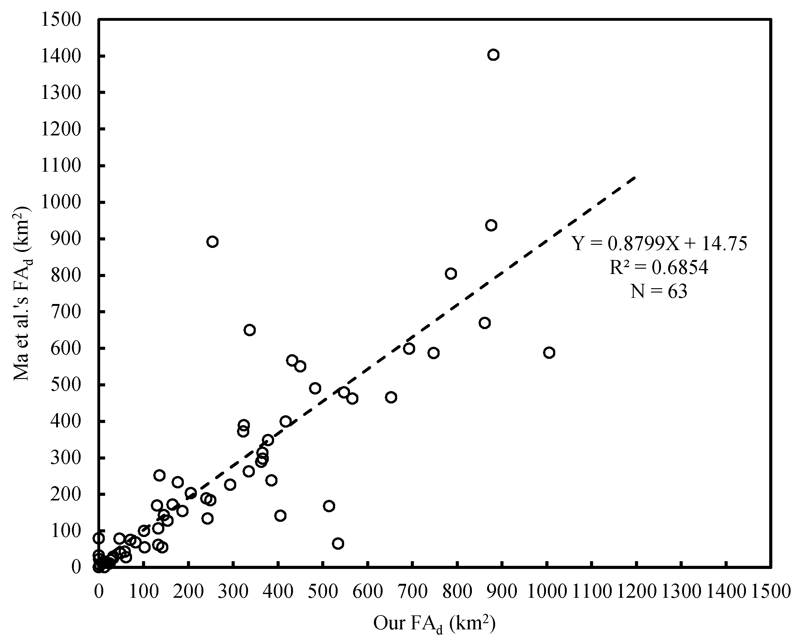
3.1.2. Validation Using the Results of Other Studies

Our monitoring workflow mainly focused on the long-term trends and dynamics of cyanobacteria blooms; therefore, large-scale patterns were, to some extent, more important than short-term and partial details. To validate our derived spatial and temporal patterns of cyanobacteria blooms, we visually inspected our results and those of other studies (

Table 3. Similar studies used for spatiotemporal pattern validation.

Reference	Indicator/Proxy	Spatial Extent	Temporal Stage
Hu et al. [15]	Cyanobacteria bloom frequency/ initial/duration/area/specific date	Entire lake	2000–2008
Duan et al. [5,34]	Cyanobacteria bloom initial date	Entire lake	1987–2011
Liu et al. [41]	Aquatic vegetation spatial/temporal dynamic	Entire lake	2003–2013
Wang et al. [2]	Chla monthly spatial dynamic	Entire lake	2002–2008
Shi et al. [26]	Chla spatial/temporal dynamic	Entire lake	2003–2013
Zhang et al. [6]	Annual and monthly cyanobacteria bloom frequency/initial date/duration	Entire lake excluding East Lake	2001-–2013

). In this process, some artifacts and a mismatch in spatiotemporal patterns were visible [39]. As a result, we found a high consistency between our spatiotemporal patterns and those of similar studies. We also extracted floating cyanobacteria corresponding to specific dates to display the evolution of the 2007 cyanobacteria blooms (Figure 4) and compared this with the results of Hu et al. [15]. We found that our long-term patterns as well as our daily spatial distribution results were highly consistent with previous reports.

In addition to the qualitative comparison between our results with others, we also quantitatively validated our findings using the Taihu Lake cyanobacteria bloom remote sensing inversion dataset (2017), which was produced and contributed by Ma et al. [5,23,57]. The dataset was supported by Lake-Watershed Science Data Center, National Earth System Science Data Sharing Infrastructure, National Science & Technology Infrastructure of China, http://lake.geodata.cn. This dataset uses the algae pixel-growing algorithm (APA), which can extract floating cyanobacteria with higher accuracy. Linear regression analysis between our results and limited FA_d data of Ma et al. in 2017 shows that there is good consistency between our results and those of Ma et al., with a linear slope close to 0.88 and a coefficient of determination (R²) close to 0.7 (Figure 5).

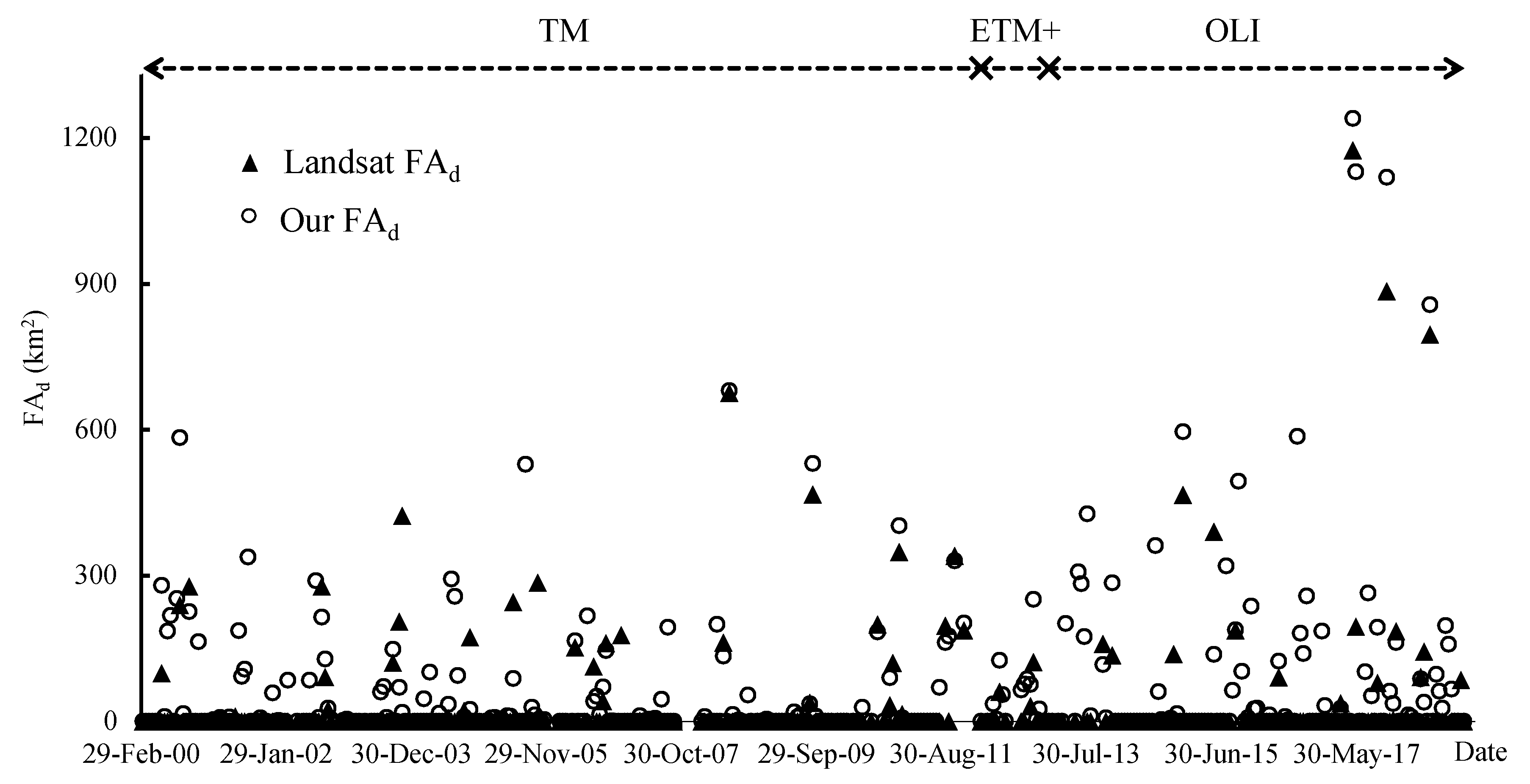
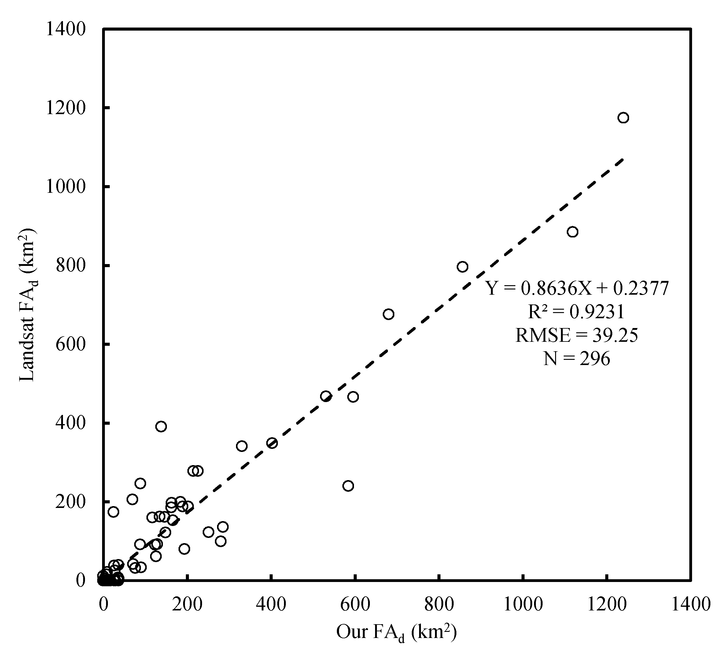
3.1.3. Validation Using Landsat Interpretation Data

Qualified Landsat images were limited due to their 16-day revisit interval and cloud contamination. We only used around 300 Landsat TM/ETM+/OLI images for validation, therefore, not every MODIS FA_d result had corresponding Landsat validation data. However, this method can be regarded as a systematic sampling process (Figure 6). Since Landsat TM/ETM+/OLI and Terra/MODIS have different local crossing times, it should be noted that wind weather or changing cloud state could affect the final consistency between the two kinds of data but, in most cases, they can retain general spatial similarity during short intervals (i.e., within a few hours). The linear regression between our FA_d and Landsat interpretation data shows there is a good correlation between the two datasets, with a linear slope equal to 0.86, R² of 0.92, and a root mean square error (RMSE) of 39.25 km² (Figure 7).

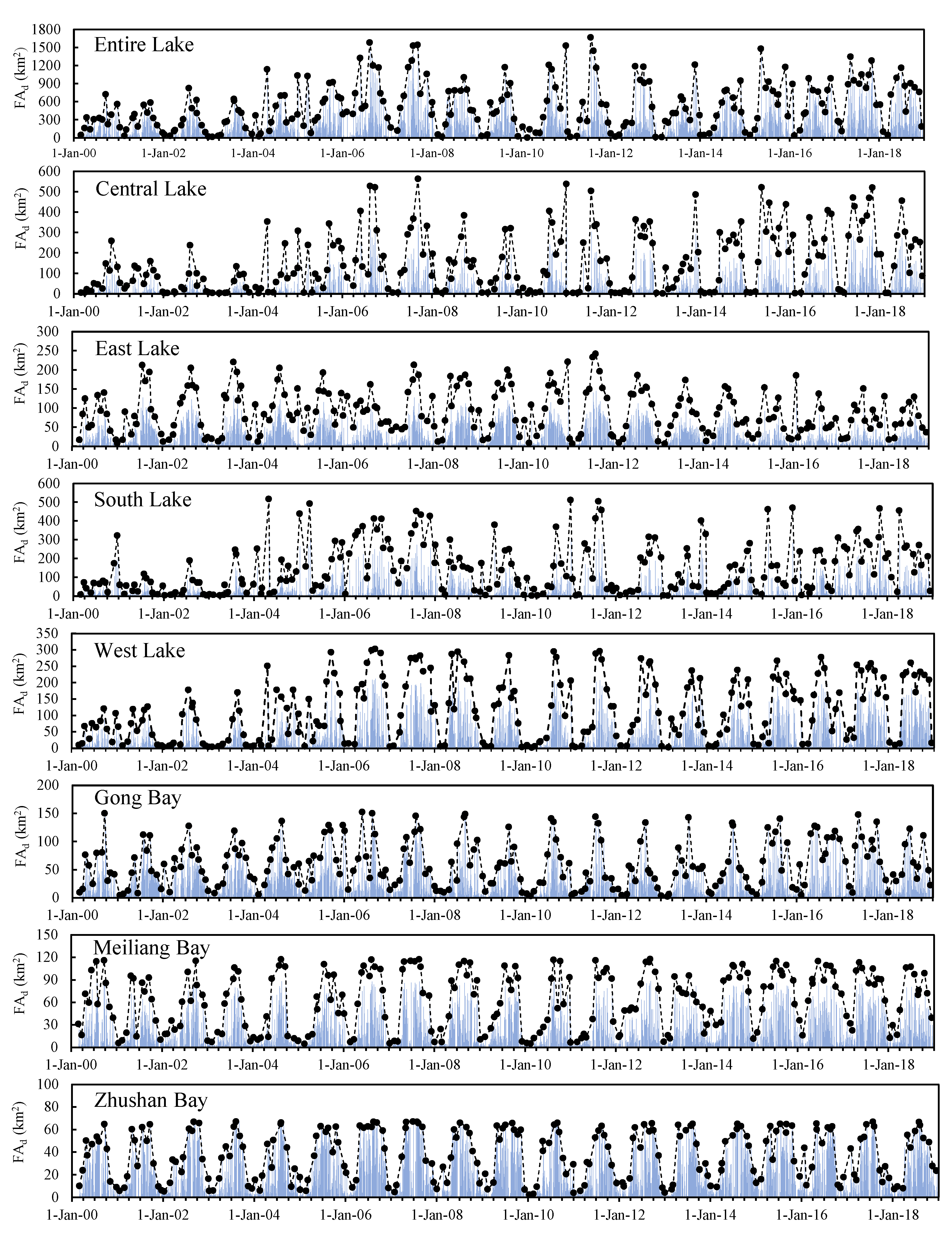
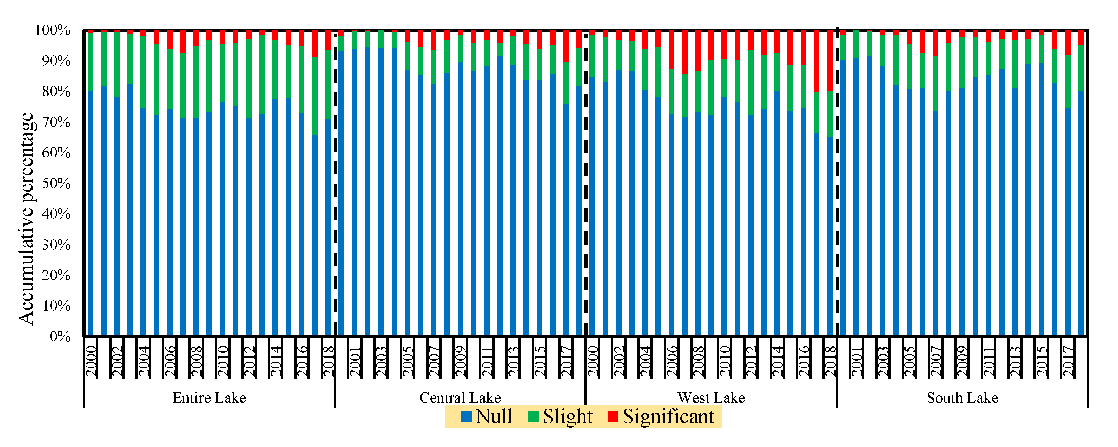
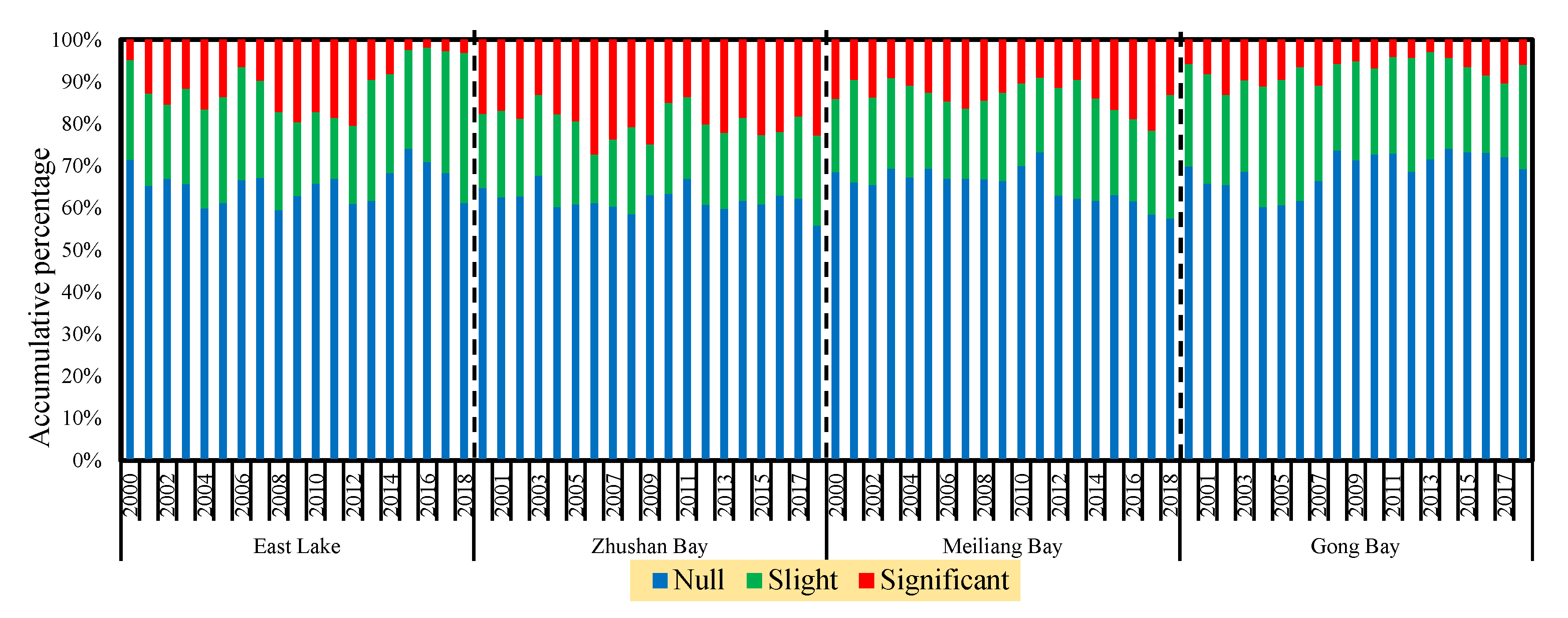
3.2. Temporal Coverage Patterns

The daily cyanobacteria bloom coverage areas (FA_d) for the entire lake (excluding East Bay) and each segment are depicted in Figure 8. Though synoptic interannual cyanobacteria bloom severity fluctuated, an obvious seasonal trend existed within each year: after a long-term bloom-free period, cyanobacteria survive and float to the water surface, relying on buoyancy. In July, August, and September, FA_d is at its largest, and individual severe cyanobacteria blooms could occur in other months. Floating cyanobacteria finally retreat during November to February of the next year. Monthly maximum FA_d is also depicted to represent the highly changeable floating cyanobacteria coverage due to the wind effect [15].

From the perspective of the entire lake, the floating cyanobacteria condition was moderate during 2000–2004. During this period, even the monthly maximum FA rarely exceeded half of the entire lake area. However, during 2005 to 2007, FA increased, in 2006 and 2007, a series of severe cyanobacteria bloom outbreaks occurred in the entire lake, which threatened the drinking water safety of the 2 million people nearby [5]. During 2008–2010, FA generally decreased. During 2011–2016, the condition fluctuated with a gradual deterioration. In 2017, a series of severe cyanobacteria blooms broke out over the entire lake over nearly the whole year. In terms of the frequency and density of floating cyanobacteria occurrence, this year’s severity level tended to overwhelm that observed in 2006 and 2007. In 2018, the condition improved but remained severe. As for Central Lake, South Lake and West Lake that occupy most of the entire lake, their FA_a dynamics were similar to that of the entire lake. As for East Lake, two obvious periods were distinguished during the long-term series: the first period was before 2013, in which FA_m and FA_a in East Lake fluctuated moderately; after 2013, the second period, FA_m and FA_a began to decrease sharply, reaching their lowest levels in 2015 and 2016, and then recovered slightly in 2017 and 2018, but to a level still less than that observed during the first period. East Lake is not as cyanobacteria-dominated as other segments and many macrophytes existed in this segment over a long period, hence its FA results could not completely represent the cyanobacteria. Three bay segments, Zhushan Bay, Meiliang Bay, and Gong Bay, are all located in the north of Taihu Lake and have bad fluid connectivity. Their FA_m and FA_a fluctuated but were relatively stable and regular over the 19 years (Figure 9). The FA results of Gong Bay were also contaminated by macrophytes, especially before 2005 (see Section 3.3). Even in some moderate years, seasons, or months, individual and serious cyanobacteria blooms still occurred, which placed heavy stress on the lake’s environment and water safety.

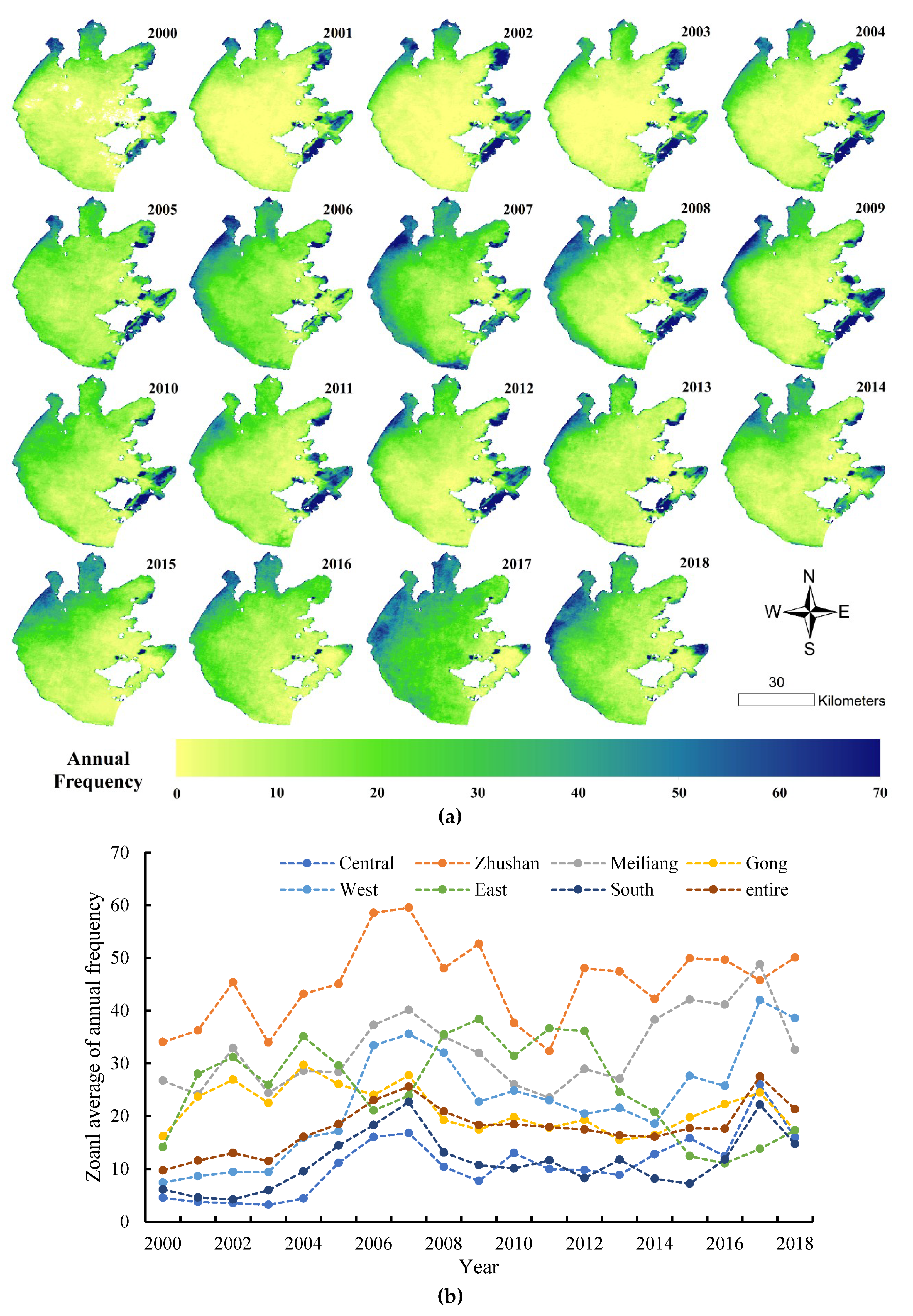
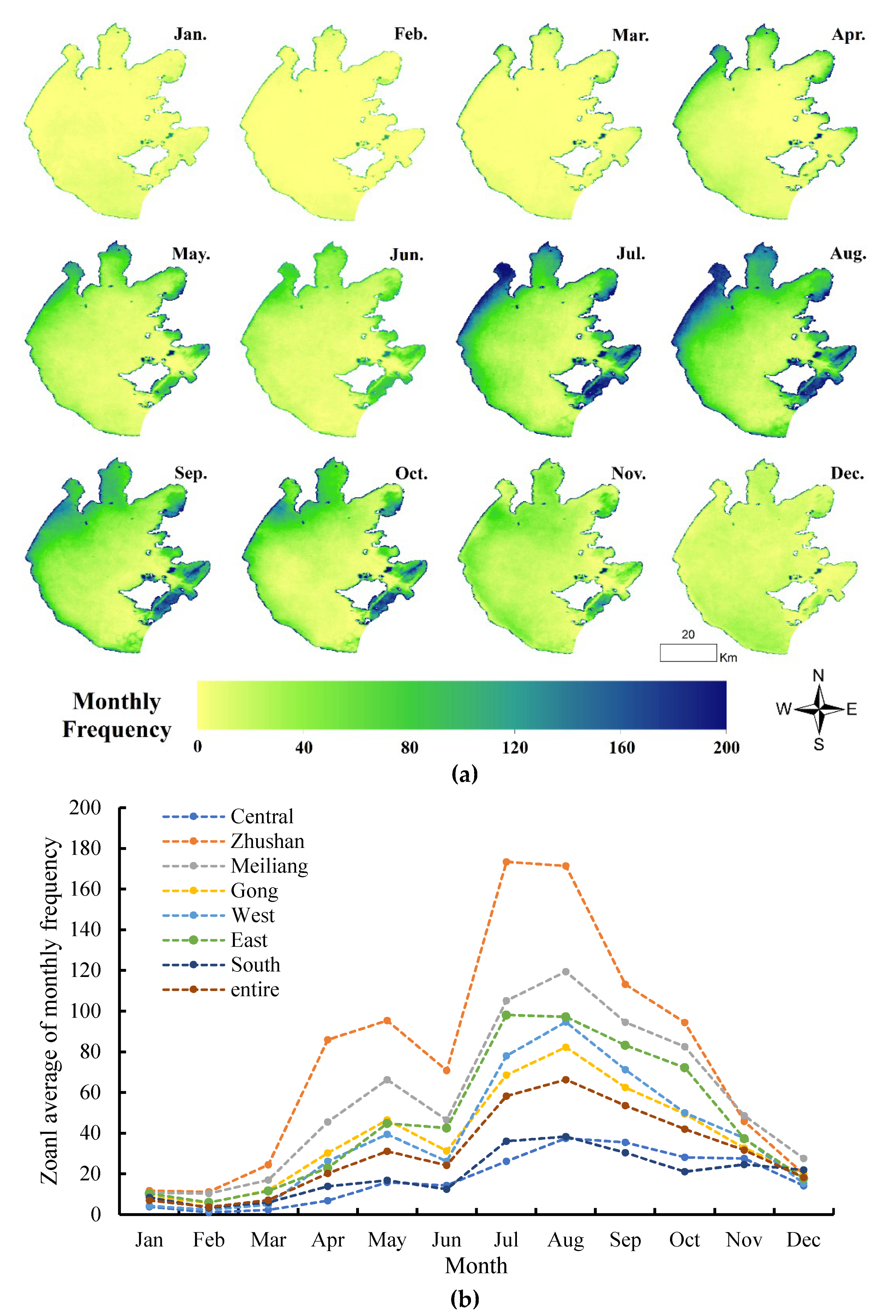
3.3. Spatial Distributions of Annual and Monthly Occurrence Frequency

According to the cyanobacteria bloom occurrence accumulative frequency (Figure 10a), between 2000 and 2005, floating cyanobacteria frequently occurred in Zhushan Bay, Meiliang Bay, and the northwest shore regions. Gong Bay and East Lake showed high occurrence frequencies; these areas were dominated by macrophytes in the beginning of 21st century [41,42,58], and we can deduce that Taihu Lake was relatively healthy in this period, excluding some bays and nearshore regions. From 2005 to 2007, cyanobacteria blooms spread from the northwest regions to the Central Lake along the shoreline. Especially in 2007, the condition was much more serious, and the bloom occurrence frequency average of 2007 was doubled in comparison to the previous several years in most lake segments (Figure 10b). Many more cyanobacteria blooms occurred in South Lake than before, and Gong Bay and East Lake’s high occurrence frequencies declined sharply. According to the findings of previous studies and the frequency-based approach [41], these segments were dominated by macrophytes, and the macrophyte ecosystems of the above two segments were destroyed due to deterioration of the water environment [42]. In 2008 and 2009, the high frequency occurrence regions gradually shrank in the northwest lake area. The increase of high frequency occurrence areas in East Lake and Gong Bay indicates that the aquatic vegetation in these segments recovered to a certain extent. During 2010 to 2014, the high occurrence regions were mainly concentrated in the northeast lake area, Zhushan Bay, and Meiliang Bay; the overall lake condition was moderate in this period. Beginning from 2015, the occurrence of high frequency tended to spread from the northwest lake area to the entire lake again, and a series of heavy cyanobacteria blooms occurred over the entire lake around 2017. The severity in this year was worse than 2007, especially in Meiliang Bay, West Lake, and Central Lake (Figure 10b). Then, the lake condition in 2018 improved slightly in most segments. We also found that in 2015, the high frequency occurrence in Gong Bay and East Lake almost disappeared and did not recover to the previous state in the following years. In 2015, the local government organized a series of mechanized salvages in East Lake and Gong Bay [42], which destroyed macrophyte roots, preventing them from participating in natural restoration.

The monthly occurrence frequencies of cyanobacteria blooms also had obvious spatial differences (Figure 11). Cyanobacteria blooms initially occurred in around April, with the occurrence locations mainly concentrated in Zhushan Bay, Meiliang Bay, Gong Bay, and the northwest nearshore regions. In summer, especially July and August, cyanobacteria blooms frequently occurred in West Lake, Zhushan Bay, and Meiliang Bay; simultaneously, Gong Bay and East Lake showed a high frequency of occurrence, mostly due to the macrophytes distributed in these areas growing rapidly in summer. From September to November, there was a gradual decrease in the coverage of high frequency; then, from December to the beginning of the next year, the floating cyanobacteria coverage was small.

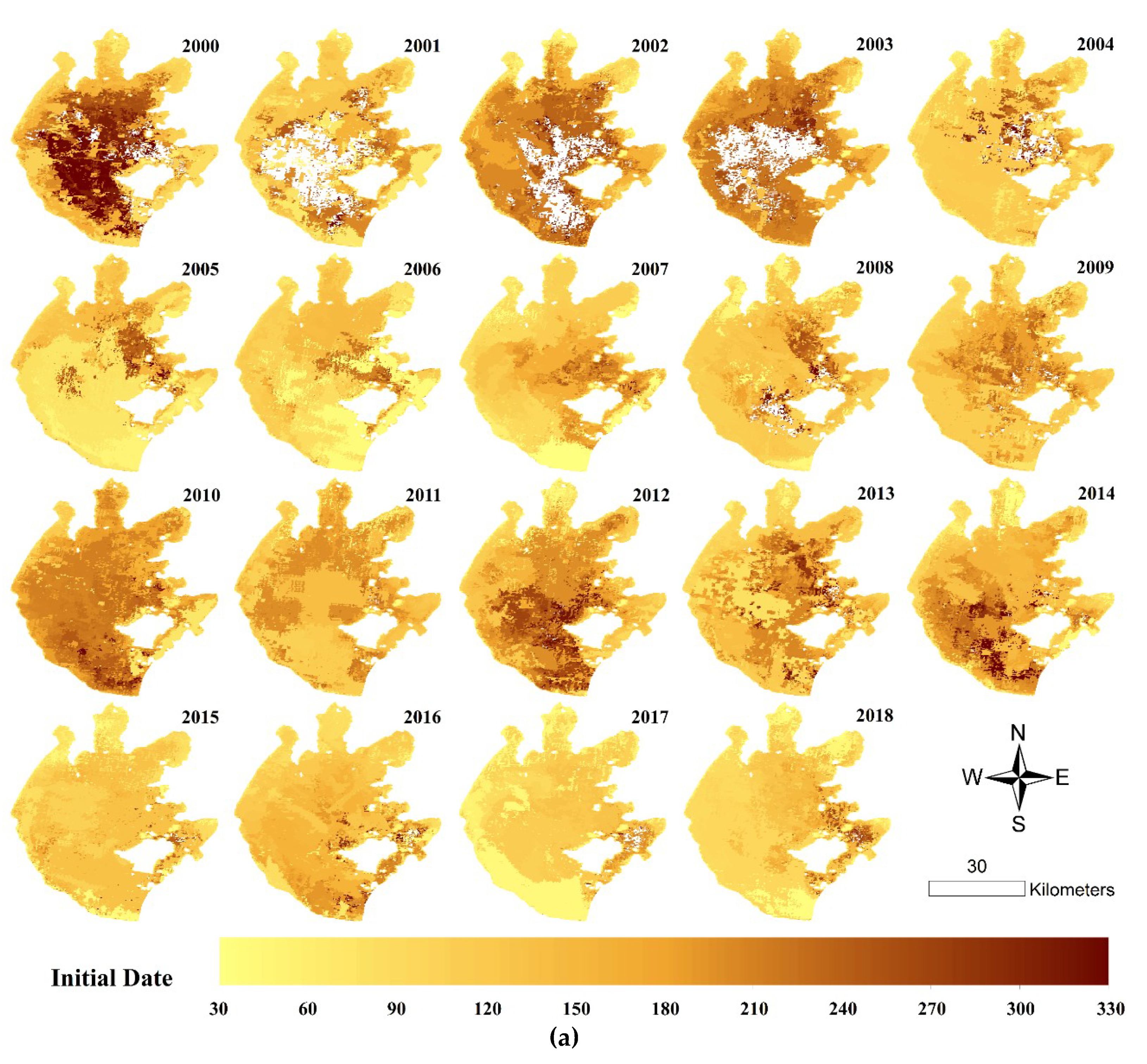
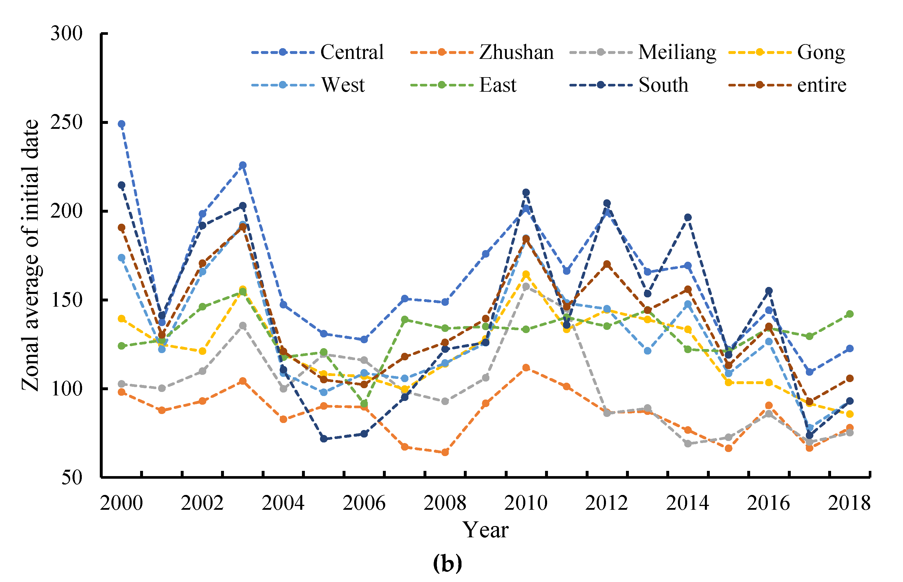
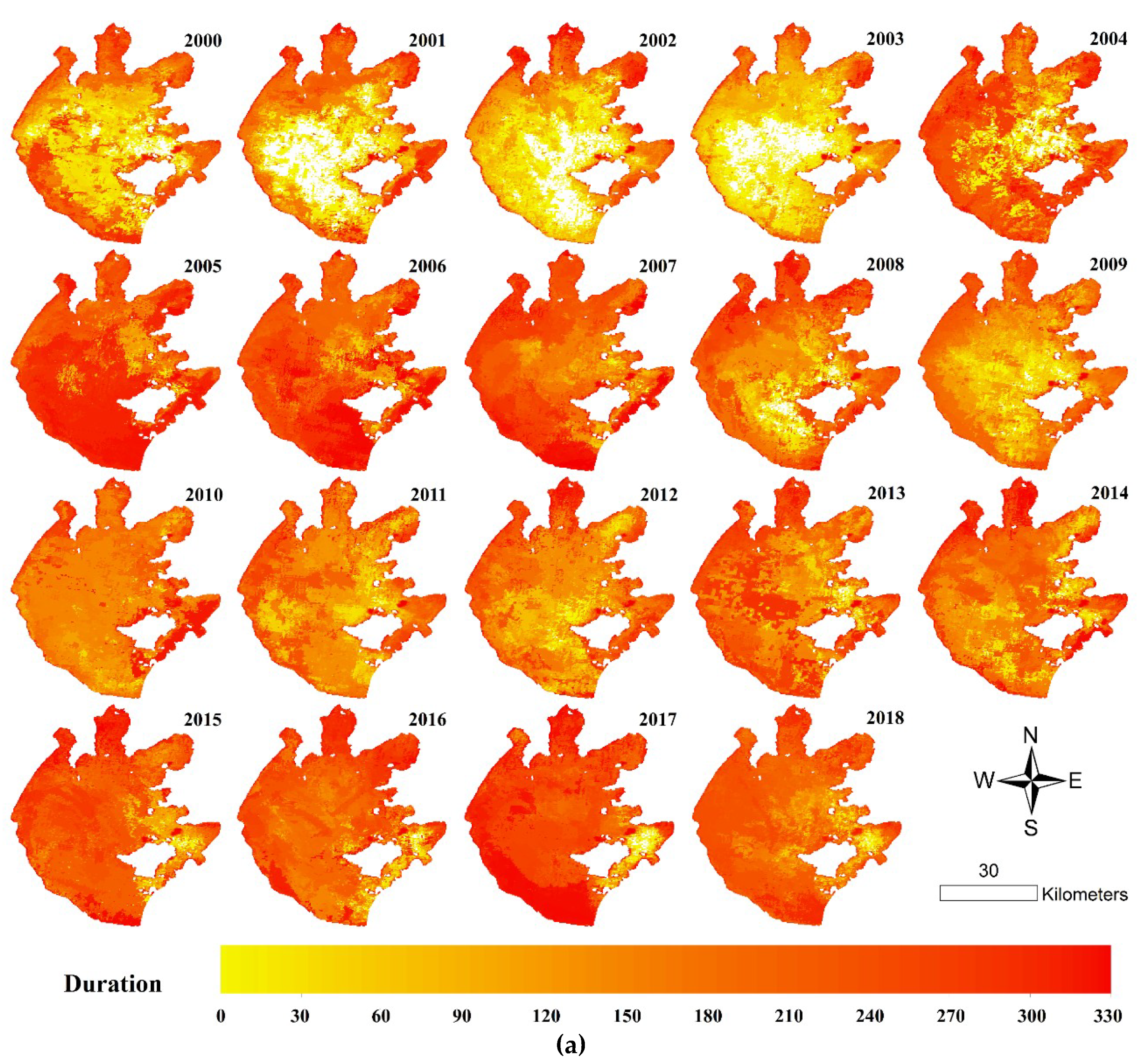
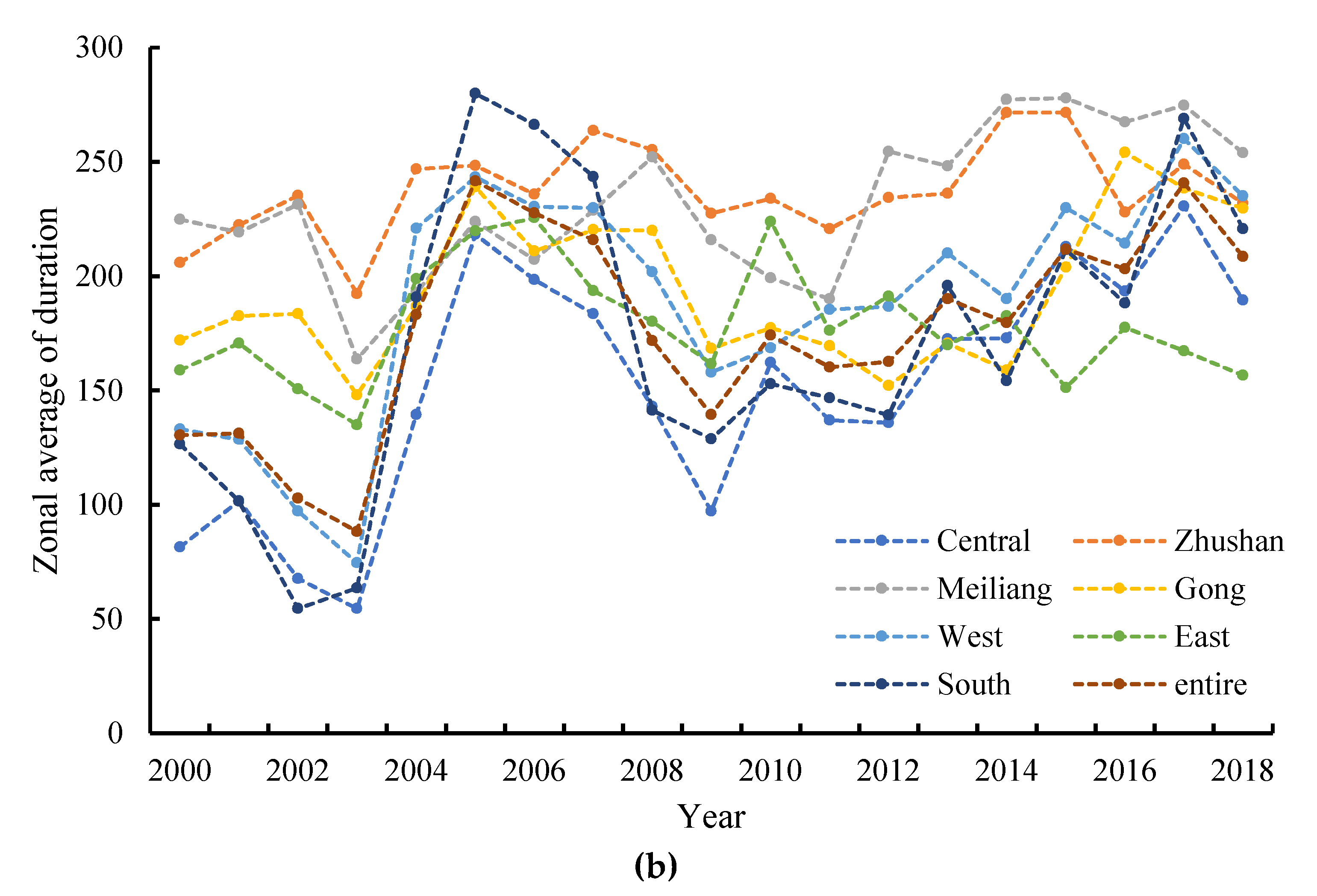
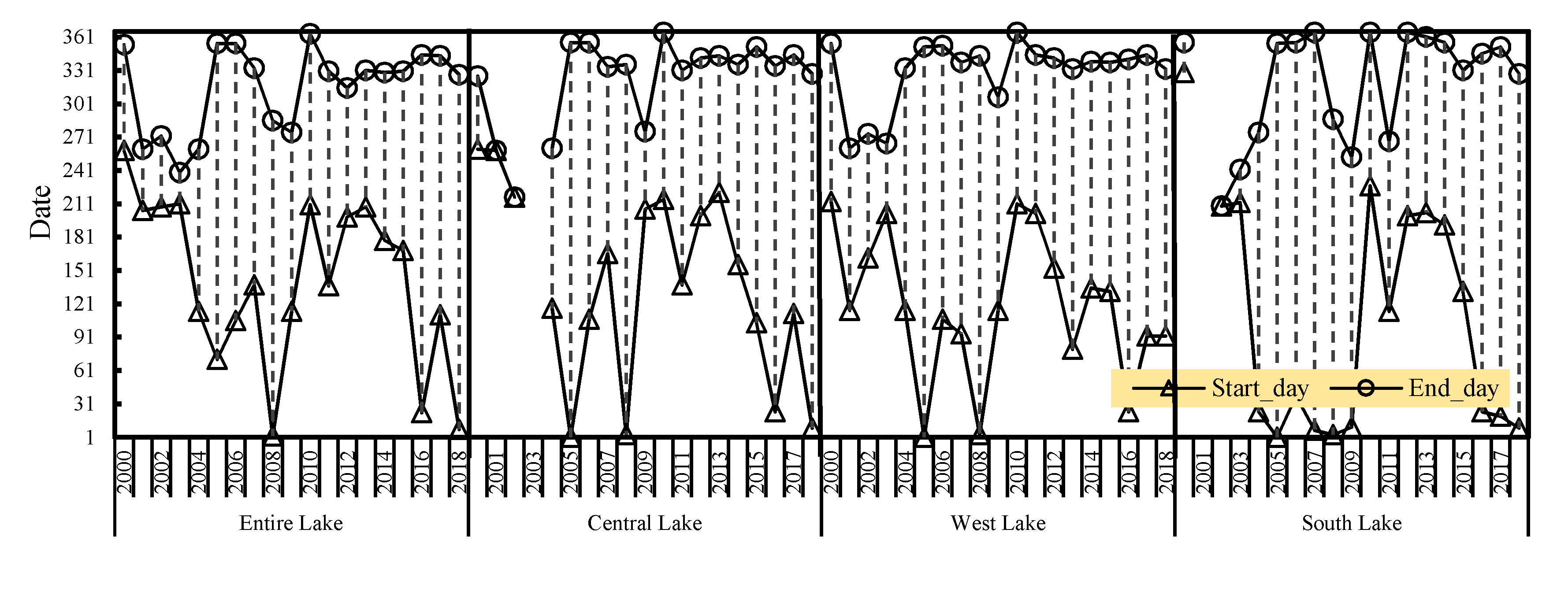
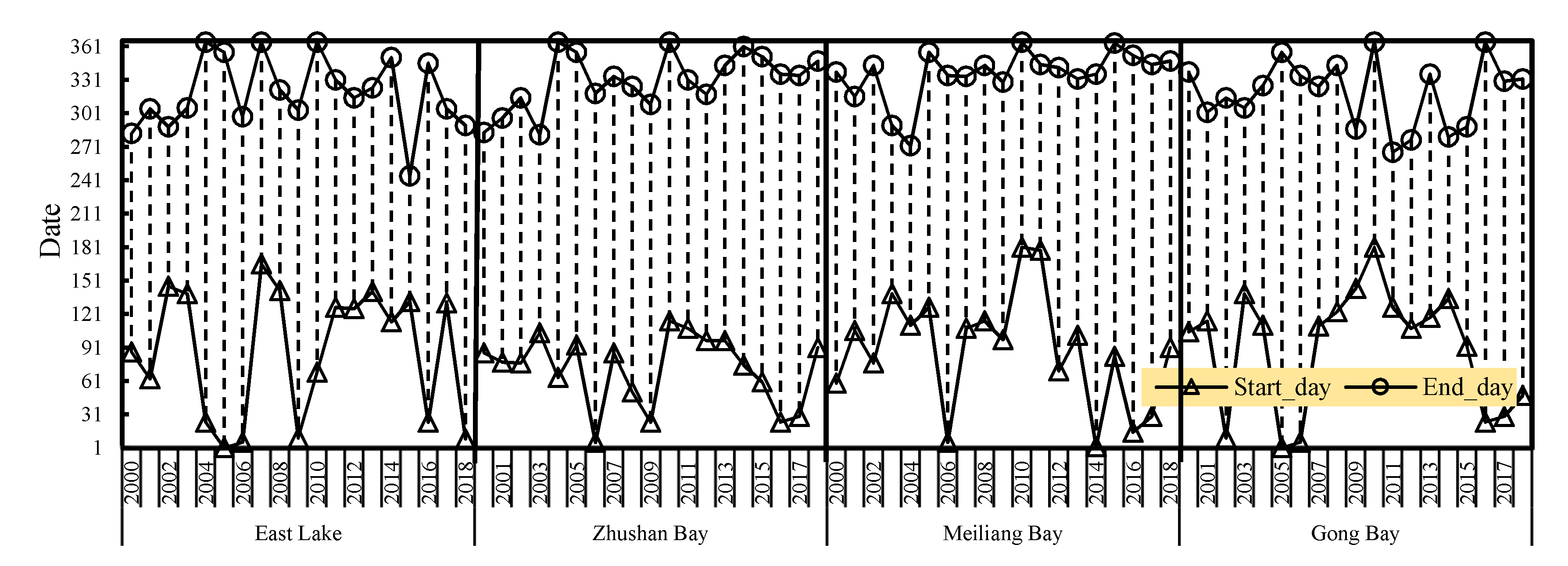
3.4. Spatial Distributions of Annual Initial Date and Duration

According to initial occurrence date of cyanobacteria blooms (Figure 12a,b), before 2004, only Zhushan Bay, Meiliang Bay, and limited nearshore areas had relatively earlier initial dates. The initial dates in most segments were considerably later, and some central lake regions did not experience cyanobacteria blooms at all. However, during 2004 to 2007, the initial date in West Lake, South Lake, and Central Lake advanced significantly. Between 2008 and 2016, the initial date of the entire lake was moderate and stable; in 2017, it advanced significantly, especially in Southwest Lake and nearshore areas. In 2018, the initial date was delayed, but in South Lake, Meiliang Bay, and Gong Bay, it was still quite early. The cyanobacteria bloom duration (Figure 13a) is the difference between the last occurrence date and the initial occurrence date, hence, in the case of the roughly stable last date, the spatial patterns of the duration were similar to the initial date, i.e., for some areas that had early (late) initial dates, their durations tended to become longer (shorter).

3.5. Temporal Characteristics of Significant Cyanobacteria Blooms

We defined significant cyanobacteria blooms as floating cyanobacteria daily coverage areas (FA_d) that exceeded 25% of the entire lake or each segment area [15], and their first and last occurrence dates are depicted in Figure 14. For the entire lake, significant cyanobacteria bloom occurrence dates were late during 2000 to 2005, advanced between 2004 to 2008, retreated between 2008 to 2015, and advanced again between 2016 to 2018. For 2008, 2016, and 2018, significant cyanobacteria blooms occurred quite early because, in the prior years, especially for 2007 and 2017, the cyanobacteria blooms were rather severe, and the early significant cyanobacteria bloom occurrence dates in 2008 and 2018 were extensions of their previous years. For open lake segments (West Lake, South Lake, and Central Lake), their significant cyanobacteria bloom occurrence dates were similar to the entire lake. For bay segments (Zhushan Bay, Meiliang Bay, and Gong Bay), their significant cyanobacteria bloom occurrence dates were earlier than the open lake segments, mainly due to severe eutrophication. The results of East Lake and Gong Bay were mixtures of cyanobacteria blooms and macrophytes, especially before 2015, when macrophytes were not being mechanically salvaged and were still prevailing.

As mentioned in the previous section, significant cyanobacteria blooms were defined as FA_d that exceeded 25% of the entire lake or each segment area. To exclude the land adjacent effect, aquatic vegetation coverage, and floating cyanobacteria extraction deviation, we regarded FA_d that was less than 5% of the entire lake (or segments) area as null floating cyanobacteria. We also defined FA_d that was greater than 5% but less than 25% of the entire lake (or segments) area as slight cyanobacteria blooms.

According to the accumulative percentage of the cyanobacteria bloom severity level (Figure 15), the entire lake experienced five stages: before 2004, significant cyanobacteria blooms rarely occurred; in 2006 and 2007, they increased rapidly; then declined in 2008; a moderate level was maintained between 2009 and 2015; and their proportion then increased after 2016. The temporal dynamics of slight cyanobacteria blooms were similar those of the significant blooms. The accumulative percentage of cyanobacteria bloom severity levels of open lake segments (West Lake, South Lake, and Central Lake) were similar to the entire lake. The periodic changes in cyanobacteria-dominated Zhushan Bay and Meiliang Bay, were similar to those observed in the entire lake, but their significant and slight severity levels occupied a greater proportion. In other words, those bays were much unhealthier than the average status. Due to much of Gong Bay’s macrophytes being vanished after 2005 [35], we deduce that the Gong Bay’s cyanobacteria bloom condition deteriorated in recent years, especially after 2015. East Lake, as a well-known macrophyte-dominated segment before 2015, demonstrated similar temporal patterns to Gong Bay.

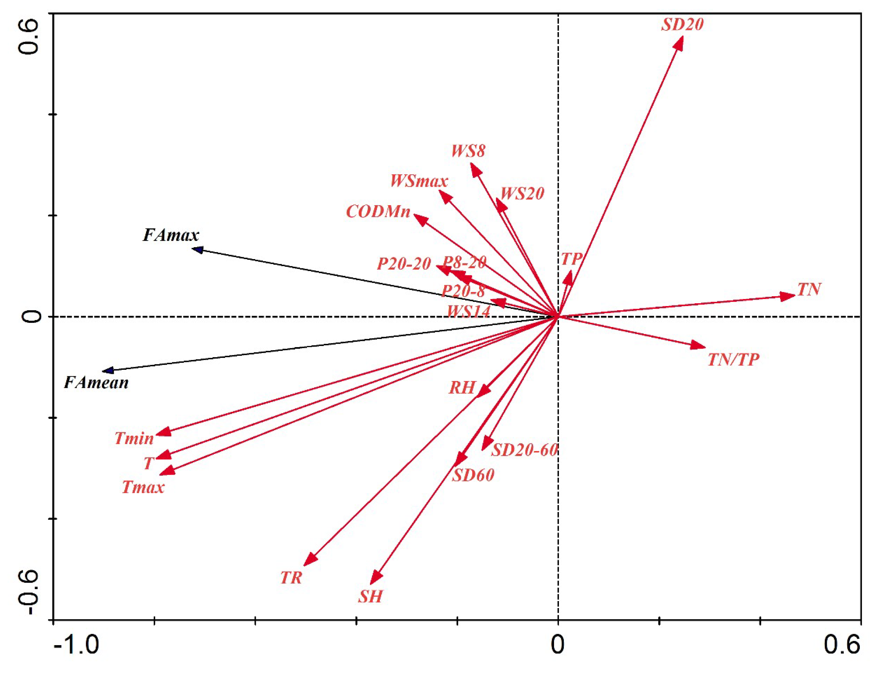
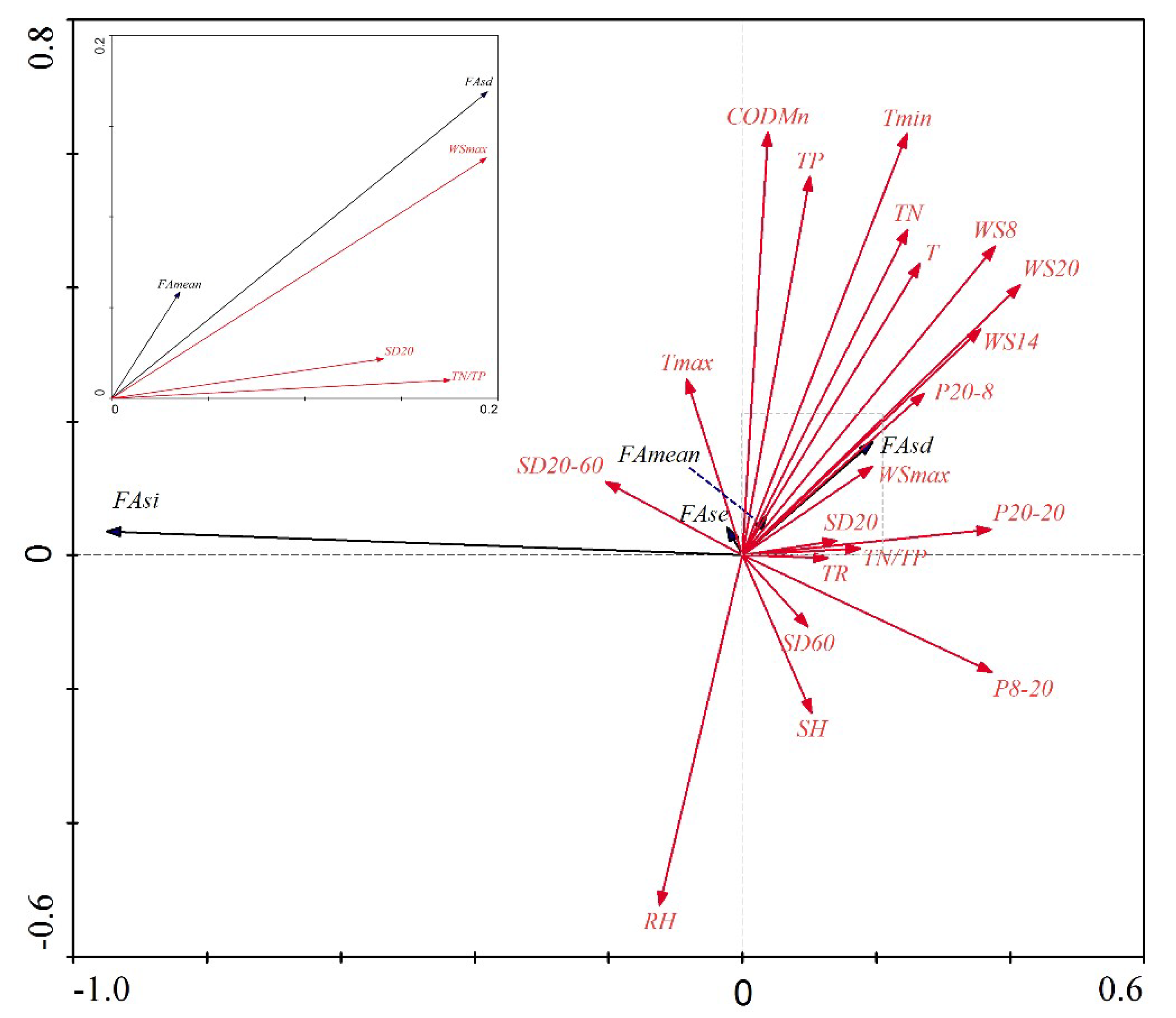
3.6. Redundancy Analysis (RDA) between Environmental Driving Factors and Cyanobacteria Bloom Characteristics

According to the monthly RDA analysis (Figure 16), temperature, sunshine radiance, wind speed, and precipitation were positively correlated with cyanobacteria blooms (both FA_mean and FA_max), but most water quality factors were negatively correlated or nearly uncorrelated with monthly cyanobacteria blooms, except COD_Mn. The T’s monthly and annual individual explanations to FA_mean were 0.273 and 0.168, respectively; while the T_min’s monthly and annual individual explanations to FA_mean were 0.283 and 0.212, respectively (

Table 4. Redundancy analysis (RDA) input variables and related statistics.

Type	Item	Abbreviation	Dimension	Monthly Permutation Test		Annual permutation Test		Individual Explanation
				P-Value 1	F-Value	P-Value	F-Value	Monthly	Annual
Meteorological factors	Monthly mean of daily mean temperature	T	°C	0.002 **	104.364	0.374	0.831	0.273	0.168
	Monthly mean of daily maximum temperature	Tmax	°C	0.002 **	101.183	0.838	0.101	0.265	0.010
	Monthly mean of daily minimum temperature	Tmin	°C	0.002 **	104.251	0.406	0.791	0.283	0.212
	Monthly mean of daily mean relative humidity	RH	%	0.140	2.525	0.644	0.256	0.015	0.117
	Monthly cumulative precipitation from 20:00 to 08:00	P20-8	mm	0.046 *	3.928	0.292	0.784	0.029	0.167
	Monthly cumulative precipitation from 08:00 to 20:00	P8-20	mm	0.040 *	4.436	0.228	1.567	0.010	0.125
	Monthly cumulative precipitation from 20:00 to 20:00	P20-20	mm	0.014 *	5.725	0.178	1.531	0.024	0.186
	Monthly amount of total radiation	TR	MJ/m2	0.002 **	29.516	0.752	0.161	0.078	0.010
	Monthly amount of sunshine hours	SH	h	0.002 **	15.073	0.778	0.129	0.034	0.008
	Monthly number of days with sunshine time greater than 60% in a day	SD60	days	0.028 *	4.239	0.848	0.098	0.006	0.002
	Monthly number of days with sunshine time less than 20% in a day	SD20	days	0.014 *	6.696	0.694	0.199	0.012	0.037
	Monthly number of days with sunshine time greater than 20% but less than 60% in a day	SD20-60	days	0.112	2.317	0.448	0.421	0.010	0.007
	Monthly maximum wind speed	WSmax	m/s	0.028 *	5.566	0.524	0.380	0.018	0.079
	Monthly mean wind speed at 08:00	WS8	m/s	0.058	3.078	0.210	1.672	0.008	0.292
	Monthly mean wind speed at 14:00	WS14	m/s	0.196	1.690	0.226	1.426	0.001	0.245
	Monthly mean wind speed at 20:00	WS20	m/s	0.216	1.533	0.136	2.059	0.006	0.286
Water quality factors	Total nitrogen	TN	mg/L	0.002 **	24.194	0.388	0.730	0.146	0.135
	Total phosphorus	TP	mg/L	0.838	0.077	0.658	0.217	0.001	0.135
	Ratio of total nitrogen to total phosphorus	TN/TP	-	0.008 **	8.432	0.634	0.318	0.079	0.021
	Chemical oxygen demand	CODMn	mg/L	0.010 **	8.247	0.748	0.168	0.066	0.110
Cyanobacteria bloom characteristics	Monthly/annual mean area of floating cyanobacteria	FAmean	km2
	Monthly maximum area of floating cyanobacteria	FAmax	km2
	Initial date of significant floating cyanobacteria	FAsi	day
	End date of significant floating cyanobacteria	FAse	day
	Duration of significant floating cyanobacteria	FAsd	days

¹ * P < 0.05, ** P < 0.01.

). Hence FA_mean had a stronger relationship with T_min than T. Previous studies have found that higher T_min in winter promotes the cyanobacteria survival over winter, and there is a significant correlation that exists between T_min and initial blooming date [5], because cyanobacteria grow better at high temperatures [59,60]. Wind speed affects FA_max more than FA_mean because wind helps cyanobacteria to form surface scum [15], especially when the wind speed is less than 4 m/s [61]. However, annual environmental variables have different effects; water quality factors, especially nutrient loadings (TN and TP)) were positively correlated with annual cyanobacteria blooms (Figure 17), probably because sporadic cyanobacteria blooms are affected by meteorological factors to a large extent, e.g., wind speed, wind direction, and temperature, but frequent and large-scale cyanobacteria blooms from the interannual perspective are dominated by nutrient distribution and abundance [7,26,62,63]. Meteorological factors were thought to play a more important role in cyanobacteria bloom formation, especially when Taihu Lake’s nutrient loadings were sufficient [64,65]. Intensive precipitation carries nutrient loadings from adjacent catchments to the lake [59], therefore, precipitation was also positively correlated with monthly and annual cyanobacteria blooms as what we got (Figure 16 and Figure 17).

4. Discussion

4.1. Accuracy Deviation Sources in Our Workflow

The validation results show that for rapid and automatic monitoring purposes, our workflow provides acceptable accuracy; however, some deviation sources remained. Firstly, compared with Rayleigh-corrected reflectance data, the MODIS land surface reflectance data (MOD09) used in our study are sensitive to ambient disturbance, which leads to some inevitable noisy, negative, or even a lack of pixel data, as well as patches [50,66]. FAI > −0.004 was used to distinguish cyanobacteria bloom pixels from non-cyanobacteria blooms [15], but no field investigation was performed to validate the accuracy using this critical threshold [15]. Liu et al. recommended FAI > −0.025 as a cyanobacteria bloom extraction threshold in Taihu Lake according to their field investigation [41]. Since most of the previous studies used FAI > −0.004 to distinguish cyanobacteria pixels in Taihu Lake, we also adopted this threshold to allow for comparison of results. FAI could just distinguish dense cyanobacteria blooms that have formed floating scums and have not mixed with the water column [15,16,52], so it is more suitable for monitoring high Chla concentration cyanobacteria blooms [13]. The FAI threshold can extract some other types of aquatic vegetation and contaminate the final statistics, including emerged and floating-leaved macrophytes, which would lead to an overestimation of cyanobacteria blooms, especially for East Lake and Gong Bay, but this deviation should not affect the long-term temporal and large-scale spatial patterns. Regardless, macrophytes distributed in the above two segments can be deduced according to previous studies and the frequency-based approach [41,58].

Another accuracy uncertainty was the land surface adjacent effect. Stray light from brighter land pixels that are adjacent to a dark water target would lead to increased radiance of NIR bands [67]; thus, the water pixels’ FAI values would be elevated according to the FAI formula, which would cause erroneous segmentation. The land surface adjacent effect may be influential for up to many kilometers offshore [67,68], but the land mask cannot be shrunk too much toward the water, under the consideration of comprehensive statistics.

Cloud contamination was another deviation source. When processing floating cyanobacteria pixels covered by thin cloud, visual inspection could be used to identify them and classify those pixels to the final floating cyanobacteria statistics, but the single-band threshold would mask thin cloud, so an underestimation of cyanobacteria blooms may have occurred in some cloudy images. The cloud mask would also remove some pixels that were contaminated by the adjacent effect, insufficient atmospheric correction, satellite sensor mechanical fault, and other accidental factors.

4.2. Environmental Driving Factors of Taihu Lake’s Severe Cyanobacteria Blooms around 2017

Massive nutrient loading input to Taihu Lake came from sewerage, agriculture fertilizer, and livestock drainage. These factors were generally considered fundamental in creating the 2007 cyanobacteria bloom crisis [5,8], which affected water safety and environment of millions of citizens. Other related environmental variables also helped to create a suitable environment for cyanobacteria bloom outbreak, e.g., temperature and wind [5,69]. After that crisis, the local government has made considerable efforts to control the nutrient loadings and pollutants enter Taihu Lake over the whole catchment. After over one decade, opposite trends were observed among some key water quality indices according to monitoring data for the entire lake: TN, NH₃-N, and COD_Mn declined rapidly after the 2007 peak, then remained at a moderate level; TP declined after the 2007 peak, then remained moderate between 2008 and 2014, rose rapidly after 2015, and reached a new peak around 2017 [36]. During the past decade, measures to control catchment pollutants have apparently been effective. However, the huge floods in 2015 and 2016 carried a huge amount of nitrogen and phosphorus to Taihu Lake. Most of the nitrogen with soluble form was discharged after the floods, but most of the phosphorus was deposited in the lake in particulate form. The reserved phosphorus that accumulated in lake sediment was gradually released by means of Microcystis growth, acidity, and oxidation changes [35]. Taihu Lake’s severe cyanobacteria blooms in 2017 were attributed to high TP concentration, high temperature, and frequent weak wind, all of which boost cyanobacteria bloom formation [70], which is consistent with our RDA analysis. The role of nitrogen is still ambiguous to some extent, some studies indicated that reducing phosphorus is more effective at causing a decline in cyanobacteria abundance [8,11,69,71,72]. We also believe that reducing TP by the means of controlling external and endogenous sources would be a feasible long-term management strategy, especially under the condition that explanation of TP was 0.135 in annual perspective, much higher than its monthly explanation (0.001) (Table 4). Long-term climate warming and wind speed decreasing over the past several decades also create a suitable environment for cyanobacteria blooms [37,59,64]. Therefore, establishing a cyanobacteria bloom monitoring system is vital towards taking preventative action in protecting water environments and safety.

As has been mentioned in above sections, FAI is not sensitive enough to distinguish between cyanobacteria and macrophyte [58], so our obtained cyanobacteria bloom spatiotemporal patterns were contaminated by macrophytes more or less, especially in East Lake and Gong Bay. Several studies have indicated that large areas of macrophytes disappeared in East Lake and Gong Bay after 2015, primarily due to mechanized salvage by the local government [42,62,73]. Taihu Lake has changed from a macrophyte-dominated state to a phytoplankton-dominated state under anthropogenic pressure [37]. The existence of an aquatic macrophyte ecosystem would help improve the underwater light environment [8], stabilize phosphorus in the sediment [73], and suppress cyanobacteria growth [74]. Local government and scientists have made great efforts to recover macrophytes; however, artificial planting and restoration in the early 2000s was unsuccessful, largely due to the water environment being unsuitable for macrophyte growth. The artificial restoration of macrophytes can only succeed when the level of nutrient loading is reduced to an appropriate level [75].

4.3. Broader Applications of Our Workflow

Inland water has more complicated inherent optical properties (IOPs) than ocean water [76]. Atmospheric correction, the adjacent effect, and other complicated inland water remote sensing problems hinder the data mining and extension of the current methodology to different research locations [77]. We embedded and integrated related processing procedures into a cloud platform (GEE), achieved an acceptable accuracy, and obtained the cyanobacteria bloom spatiotemporal patterns of Taihu Lake. We believe our workflow has the potential to be applied to other lakes and coastal waters for similar purposes. Researchers should attempt to embed different atmospheric correction algorithms and cyanobacteria bloom extraction methods for different inland waters when using our workflow.

The floating cyanobacteria coverage we extracted can only represent the horizontal distribution, but not the cyanobacteria biomass, which must consider the vertical distribution of cyanobacteria biomass in the water column. Thus, related remote sensing inversion algorithms may be embedded into our workflow in future. The FAI threshold method in our workflow could potentially be improved by the algae pixel-growing algorithm (APA) [57] or the histogram adaptive threshold, etc. Overall, further efforts are urgently required to embed many types of conventional inversion algorithms and operational processes into cloud platforms, which will help us find new information by combining remote sensing big data and specific natural or social scenarios.

5. Conclusions

In this study, we developed an operational cyanobacteria bloom monitoring workflow based on Google Earth Engine, processed nearly 7000 MODIS daily images, and retrieved spatial and temporal patterns of cyanobacteria blooms in China’s Taihu Lake, over 19 years (2000 to 2018). Our workflow provides a basis for automatic remote sensing monitoring of cyanobacteria blooms. Several conclusions were reached in our study:

(1) Some sources of error in our workflow were reported, such as the FAI threshold, the land surface adjacent effect, and cloud contamination. However, inspected by the validation using in-situ data and remote sensing observations, the workflow still achieved an acceptable accuracy for rapid and automatic monitoring purposes. Our workflow can improve the automation and efficiency of routine environmental management of Taihu Lake and has the potential to be applied to other inland and coastal water areas.

(2) From the perspective of temporal coverage distribution, cyanobacteria blooms in Taihu Lake were moderate before 2006, peaked in 2007, declined rapidly after 2008, remained moderate and stable until 2015, and then reached another peak around 2017. Several lake segments displayed similar temporal trends to the entire lake, especially for those open lake segments. From the perspective of interannual spatial distribution, bay areas and the northwest lake area had more severe cyanobacteria blooms than open lake segments. From the perspective of monthly spatial distribution, most cyanobacteria blooms primarily occurred in April, became severe in July and August, then improved after October. We also found that macrophytes distributed in East Lake and Gong Bay disappeared after 2015 and have not yet been restored.

(3) According to the redundancy analysis, meteorological factors (temperature, wind speed, precipitation, etc.) were positively correlated with cyanobacteria bloom characteristics, from both monthly and interannual perspectives; however, nutrient loadings were only positively correlated with cyanobacteria bloom characteristics from an annual perspective. Reducing total phosphorous (TP) by controlling external and endogenous sources, together with restoring macrophyte ecosystem, would be the feasible long-term management strategies for Taihu Lake.

References

1. Sellner, K.G.; Doucette, G.J.; Kirkpatrick, G.J. Harmful algal blooms: Causes, impacts and detection. J. Ind. Microbiol. Biotechnol. 2003, 30, 383–406. [Google Scholar] [CrossRef] [PubMed]
2. Wang, M.; Shi, W.; Tang, J. Water property monitoring and assessment for China’s inland Lake Taihu from MODIS-Aqua measurements. Remote Sens. Environ. 2011, 115, 841–854. [Google Scholar] [CrossRef]
3. Kudela, R.M.; Palacios, S.L.; Austerberry, D.C.; Accorsi, E.K.; Guild, L.S.; Torres-Perez, J. Application of hyperspectral Remote Sensing to cyanobacterial blooms in inland waters. Remote Sens. Environ. 2015, 167, 196–205. [Google Scholar] [CrossRef]
4. Blondeau-Patissier, D.; Gower, J.F.R.; Dekker, A.G.; Phinn, S.R.; Brando, V.E. A review of ocean color Remote Sensing methods and statistical techniques for the detection, mapping and analysis of phytoplankton blooms in coastal and open oceans. Progr. Oceanogr. 2014, 123, 123–144. [Google Scholar] [CrossRef]
5. Duan, H.; Ma, R.; Xu, X.; Kong, F.; Zhang, S.; Kong, W.; Hao, J.; Shang, L. Two-Decade Reconstruction of Algal Blooms in China’s Lake Taihu. Environ. Sci. Technol. 2009, 43, 3522–3528. [Google Scholar] [CrossRef]
6. Zhang, Y.; Ma, R.; Duan, H.; Loiselle, S.; Xu, J. Satellite analysis to identify changes and drivers of CyanoHABs dynamics in Lake Taihu. Water Sci. Technol. Water Suppl. 2016, 16, 1451–1466. [Google Scholar] [CrossRef]
7. Chen, Y.; Qin, B.; Teubner, K.; Dokulil, M.T. Long-term dynamics of phytoplankton assemblages: Microcystis-domination in Lake Taihu, a large shallow lake in China. J. Plankton Res. 2003, 25, 445–453. [Google Scholar]
8. Zhang, M.; Shi, X.; Yang, Z.; Yu, Y.; Shi, L.; Qin, B. Long-term dynamics and drivers of phytoplankton biomass in eutrophic Lake Taihu. Sci. Total Environ. 2018, 645, 876–886. [Google Scholar] [CrossRef]
9. Qin, B.; Yang, G.; Ma, J.; Wu, T.; Li, W.; Liu, L.; Deng, J.; Zhou, J. Spatiotemporal Changes of Cyanobacterial Bloom in Large Shallow Eutrophic Lake Taihu, China. Front Microbiol. 2018, 9, 451. [Google Scholar] [CrossRef]
10. Peretyatko, A.; Teissier, S.; Backer, S.D.; Triest, L. Assessment of the risk of cyanobacterial bloom occurrence in urban ponds: Probabilistic approach. Annal. Limnolog. Int. J. Limnol. 2010, 46, 121–133. [Google Scholar] [CrossRef]
11. Descy, J.P.; Leprieur, F.; Pirlot, S.; Leporcq, B.; Van Wichelen, J.; Peretyatko, A.; Teissier, S.; Codd, G.A.; Triest, L.; Vyverman, W.; et al. Identifying the factors determining blooms of cyanobacteria in a set of shallow lakes. Ecol. Inform. 2016, 34, 129–138. [Google Scholar] [CrossRef]
12. Rigosi, A.; Hanson, P.; Hamilton, D.P.; Hipsey, M.; Rusak, J.A.; Bois, J.; Sparber, K.; Chorus, I.; Watkinson, A.J.; Qin, B.; et al. Determining the probablity of cyanobacteria blooms: the application of Bayesian networks in multiple lake systems. Ecol. Appl. 2015, 25, 186–199. [Google Scholar] [CrossRef] [PubMed]
13. Oyama, Y.; Fukushima, T.; Matsushita, B.; Matsuzaki, H.; Kamiya, K.; Kobinata, H. Monitoring levels of cyanobacterial blooms using the visual cyanobacteria index (VCI) and floating algae index (FAI). Int. J. Appl. Earth Observ. Geoinform. 2015, 38, 335–348. [Google Scholar] [CrossRef]
14. Kuster, T. Quantitative detection of chlorophyll in cynaobacteria bloom by satellite. Remote Sens. Limnol. Oceanogr. 2004, 49, 2179–2189. [Google Scholar]
15. Hu, C.; Lee, Z.; Ma, R.; Yu, K.; Li, D.; Shang, S. Moderate Resolution Imaging Spectroradiometer (MODIS) observations of cyanobacteria blooms in Taihu Lake, China. J. Geophys. Res. Oceans 2010, 115. [Google Scholar] [CrossRef] [Green Version]
16. Hu, C. A novel ocean color index to detect floating algae in the global oceans. Remote Sens. Environ. 2009, 113, 2118–2129. [Google Scholar] [CrossRef]
17. Zhang, Y.; Feng, L.; Li, J.; Luo, L.; Yin, Y.; Liu, M.; Li, Y. Seasonal-spatial variation and Remote Sensing of phytoplankton absorption in Lake Taihu, a large eutrophic and shallow lake in China. J. Plankton Res. 2010, 32, 1023–1037. [Google Scholar] [CrossRef]
18. Duan, H.; Ma, R.; Hu, C. Evaluation of Remote Sensing algorithms for cyanobacterial pigment retrievals during spring bloom formation in several lakes of East China. Remote Sens. Environ. 2012, 126, 126–135. [Google Scholar] [CrossRef]
19. Hu, C. An empirical approach to derive MODIS ocean color patterns under severe sun glint. Geophys. Res. Lett. 2011, 38. [Google Scholar] [CrossRef]
20. Feng, L.; Hu, C.; Chen, X.; Cai, X.; Tian, L.; Gan, W. Assessment of inundation changes of Poyang Lake using MODIS observations between 2000 and 2010. Remote Sens. Environ. 2012, 121, 80–92. [Google Scholar] [CrossRef]
21. Hu, C.; Li, D.; Chen, C.; Ge, J.; Muller-Karger, F.E.; Liu, J.; Yu, F.; He, M.-X. On the recurrent Ulva prolifera blooms in the Yellow Sea and East China Sea. J. Geophys. Res. Oceans 2010, 115. [Google Scholar] [CrossRef]
22. Huang, C.; Li, Y.; Yang, H.; Sun, D.; Yu, Z.; Zhang, Z.; Chen, X.; Xu, L. Detection of algal bloom and factors influencing its formation in Taihu Lake from 2000 to 2011 by MODIS. Environ. Earth Sci. 2013, 71, 3705–3714. [Google Scholar] [CrossRef]
23. Zhang, Y.; Ma, R.; Zhang, M.; Duan, H.; Loiselle, S.; Xu, J. Fourteen-Year Record (2000–2013) of the Spatial and Temporal Dynamics of Floating Algae Blooms in Lake Chaohu, Observed from Time Series of MODIS Images. Remote Sens. 2015, 7, 10523–10542. [Google Scholar] [CrossRef]
24. Kabenge, M.; Wang, H.; Li, F. Urban eutrophication and its spurring conditions in the Murchison Bay of Lake Victoria. Environ. Sci. Pollut. Res. Int. 2016, 23, 234–241. [Google Scholar] [CrossRef] [PubMed]
25. Wang, M.; Hu, C. Mapping and quantifying Sargassum distribution and coverage in the Central West Atlantic using MODIS observations. Remote Sens. Environ. 2016, 183, 350–367. [Google Scholar] [CrossRef]
26. Shi, K.; Zhang, Y.; Zhou, Y.; Liu, X.; Zhu, G.; Qin, B.; Gao, G. Long-term MODIS observations of cyanobacterial dynamics in Lake Taihu: Responses to nutrient enrichment and meteorological factors. Sci. Rep. 2017, 7, 40326. [Google Scholar] [CrossRef] [PubMed] [Green Version]
27. Gorelick, N.; Hancher, M.; Dixon, M.; Ilyushchenko, S.; Thau, D.; Moore, R. Google Earth Engine: Planetary-scale geospatial analysis for everyone. Remote Sens. Environ. 2017, 202, 18–27. [Google Scholar] [CrossRef]
28. Murphy, S.; Wright, R.; Rouwet, D. Color and temperature of the crater lakes at Kelimutu volcano through time. Bull. Volcanol. 2017, 80. [Google Scholar] [CrossRef]
29. Griffin, C.G.; McClelland, J.W.; Frey, K.E.; Fiske, G.; Holmes, R.M. Quantifying CDOM and DOC in major Arctic rivers during ice-free conditions using Landsat TM and ETM+ data. Remote Sens. Environ. 2018, 209, 395–409. [Google Scholar] [CrossRef]
30. Lin, S.; Novitski, L.N.; Qi, J.; Stevenson, R.J. Landsat TM/ETM+ and Machine-Learning Algorithms for Limnological Studies and algal Bloom Management of Inland Lakes; SPIE: Bellingham, WA, USA, 2018; Volume 12, pp. 1–17. [Google Scholar]
31. Traganos, D.; Aggarwal, B.; Poursanidis, D.; Topouzelis, K.; Chrysoulakis, N.; Reinartz, P. Towards Global-Scale Seagrass Mapping and Monitoring Using Sentinel-2 on Google Earth Engine: The Case Study of the Aegean and Ionian Seas. Remote Sens. 2018, 10, 1227. [Google Scholar] [CrossRef]
32. Traganos, D.; Poursanidis, D.; Aggarwal, B.; Chrysoulakis, N.; Reinartz, P. Estimating Satellite-Derived Bathymetry (SDB) with the Google Earth Engine and Sentinel-2. Remote Sens. 2018, 10, 859. [Google Scholar] [CrossRef]
33. Chen, J.; Quan, W.; Zhang, M.; Cui, T. A Simple Atmospheric Correction Algorithm for MODIS in Shallow Turbid Waters: A Case Study in Taihu Lake. IEEE J. Sel. Topics Appl. Earth Observ. Remote Sens. 2013, 6, 1825–1833. [Google Scholar] [CrossRef]
34. Duan, H.; Ma, R.; Zhang, Y.; Loiselle, S.A. Are algal blooms occurring later in Lake Taihu? Climate local effects outcompete mitigation prevention. J. Plankton Res. 2014, 36, 866–871. [Google Scholar] [CrossRef] [Green Version]
35. Zhu, W.; Tan, Y.; Wang, R.; Feng, G.; Chen, H.; Liu, Y.; Li, M. The trend of water quality variation and analysis in typical area Lake Taihu, 2010-2017. J. Lake Sci. 2018, 30, 296–305. [Google Scholar] [CrossRef]
36. Gu, X.; Zeng, Q.; Mao, Z.; Chen, H.; Li, H. Water environment change over the period 2007 - 2016 and the strategy of fishery improve the water quality of Lake Taihu. J. Lake Sci. 2019, 31, 305–318. [Google Scholar] [CrossRef]
37. Shi, K.; Zhang, Y.; Zhang, Y.; Li, N.; Qin, B.; Zhu, G.; Zhou, Y. Phenology of Phytoplankton Blooms in a Trophic Lake Observed from Long-Term MODIS Data. Environ. Sci. Technol. 2019, 53, 2324–2331. [Google Scholar] [CrossRef] [PubMed]
38. Huang, L.; Fang, H.; He, G.; Jiang, H.; Wang, C. Effects of internal loading on phosphorus distribution in the Taihu Lake driven by wind waves and lake currents. Environ. Pollut. 2016, 219, 760–773. [Google Scholar] [CrossRef]
39. Li, J.; Hu, C.; Shen, Q.; Barnes, B.B.; Murch, B.; Feng, L.; Zhang, M.; Zhang, B. Recovering low quality MODIS-Terra data over highly turbid waters through noise deduction and regional vicarious calibratioin adjustment: A case study in Taihu Lake. Remote Sens. Environ. 2017, 197, 72–84. [Google Scholar] [CrossRef]
40. Jiang, G.; Ma, R.; Loiselle, S.A.; Duan, H.; Su, W.; Cai, W.; Huang, C.; Yang, J.; Yu, W. Remote Sensing of particulate organic carbon dynamics in a eutrophic lake (Taihu Lake, China). Sci. Total. Environ. 2015, 532, 245–254. [Google Scholar] [CrossRef]
41. Liu, X.; Zhang, Y.; Shi, K.; Zhou, Y.; Tang, X.; Zhu, G.; Qin, B. Mapping Aquatic Vegetation in a Large, Shallow Eutrophic Lake: A Frequency-Based Approach Using Multiple Years of MODIS Data. Remote Sens. 2015, 7, 10295–10320. [Google Scholar] [CrossRef] [Green Version]
42. Wang, S.; Gao, Y.; Li, Q.; Gao, J.; Zhai, S.; Zhou, Y.; Cheng, Y. Long-term and inter-monthly dynamics of aquatic vegetation and its relation with environmental factors in Taihu Lake, China. Sci. Total Environ. 2019, 651, 367–380. [Google Scholar] [CrossRef] [PubMed]
43. Vermote, E.W.; Wolfe, R. MOD09GQ MODIS/Terra Surface Reflectance Daily L2G Global 250m SIN Grid V006 [Data set]. NASA EOSDIS LP DAAC 2015. [Google Scholar] [CrossRef]
44. Vermote, E.W. MODIS/Terra Surface Reflectance Daily L2G Global 1kmand 500m SIN Grid V006 [Data set]. NASA EOSDIS LP DAAC 2015. [Google Scholar] [CrossRef]
45. Wang, S. Tropical state assessment of global inland waters using a MODIS-derived Forel-Ule index. Remote Sens. Environ. 2018. [Google Scholar] [CrossRef]
46. Liu, R.; Liu, Y. Generation of new cloud masks from MODIS land surface reflectance products. Remote Sens. Environ. 2013, 133, 21–37. [Google Scholar] [CrossRef]
47. Chen, P.Y.; Srinivasan, R.; Fedosejevs, G.; Narasimhan, B. An automated cloud detection method for daily NOAA-14 AVHRR data for Texas, USA. Int. J. Remote Sens. 2002, 23, 2939–2950. [Google Scholar] [CrossRef]
48. Chen, Z.; Hu, C.; Muller-Karger, F. Monitoring turbidity in Tampa Bay using MODIS/Aqua 250-m imagery. Remote Sens. Environ. 2007, 109, 207–220. [Google Scholar] [CrossRef]
49. Wang, S.; Li, J.; Zhang, B.; Shen, Q.; Zhang, F.; Lu, Z. A simple correction method for the MODIS surface reflectance product over typical inland waters in China. Int. J. Remote Sens. 2016, 37, 6076–6096. [Google Scholar] [CrossRef]
50. Feng, L.; Hu, C.; Li, J. Can MODIS Land Reflectance Products be Used for Estuarine and Inland Waters? Water Resour. Res. 2018, 54, 3583–3601. [Google Scholar] [CrossRef]
51. Wang, S.; Yang, M.; Li, J.; Shen, Q.; Zhang, F. MODIS surface reflectance product (MOD09) validation for typical inland waters in China. SPIE Proc. 2014, 9261, 92610F. [Google Scholar] [CrossRef]
52. Moradi, M. Comparison of the efficacy of MODIS and MERIS data for detecting cyanobacterial blooms in the southern Caspian Sea. Mar. Pollut. Bull. 2014, 87, 311–322. [Google Scholar] [CrossRef] [PubMed]
53. Legendre, P.; Anderson, M.J. Distance-based redundancy analysis: Testing multispecies responses in multifactorial ecological experiments. Ecol. Monogr. 1999, 69, 1–24. [Google Scholar] [CrossRef]
54. Legendre, P.; Gallagher, E.D. Ecologically meaningful transformations for ordination of species data. Oecologia 2001, 129, 271–280. [Google Scholar] [CrossRef] [PubMed]
55. Chen, S.; Zhang, W.; Zhang, J.; Jeppesen, E.; Liu, Z.; Kociolek, J.P.; Xu, X.; Wang, L. Local habitat heterogeneity determines the differences in benthic diatom metacommunities between different urban river types. Sci. Total. Environ. 2019, 669, 711–720. [Google Scholar] [CrossRef]
56. Huang, Y.; Huang, J. Coupled effects of land use pattern and hydrological regime on composition and diversity of riverine eukaryotic community in a coastal watershed of Southeast China. Sci. Total. Environ. 2019, 660, 787–798. [Google Scholar] [CrossRef] [PubMed]
57. Zhang, Y.; Ma, R.; Duan, H.; Loiselle, S.A.; Xu, J.; Ma, M. A novel algorithm to estimate algae bloom coverage to subpixel resolution in Taihu Lake. IEEE J. Sel. Topics Appl. Earth Observ. Remote Sens. 2014, 7, 3060–3068. [Google Scholar] [CrossRef]
58. Liang, Q.; Zhang, Y.; Ma, R.; Loiselle, S.; Li, J.; Hu, M. A MODIS-Based Novel Method to Distinguish Surface Cyanobacterial Scums and Aquatic Macrophytes in Lake Taihu. Remote Sens. 2017, 9, 133. [Google Scholar] [CrossRef]
59. Paerl, H.W.; Huisman, J. Bloom Like It Hot. Science 2008, 320, 57–58. [Google Scholar] [CrossRef] [PubMed]
60. Visser, P.M.; Verspagen, J.M.H.; Sandrini, G.; Stal, L.J.; Matthijs, H.C.P.; Davis, T.W.; Paerl, H.W.; Huisman, J. How rising CO2 and global warming may stimulate harmful cyanobacterial blooms. Harmful Algae 2016, 54, 145–159. [Google Scholar] [CrossRef]
61. Cao, H.-S.; Kong, F.-X.; Luo, L.-C.; Shi, X.-L.; Yang, Z.; Zhang, X.-F.; Tao, Y. Effects of Wind and Wind-Induced Waves on Vertical Phytoplankton Distribution and Surface Blooms ofMicrocystis aeruginosain Lake Taihu. J. Freshw. Ecol. 2006, 21, 231–238. [Google Scholar] [CrossRef]
62. Zhang, M.; Yang, Z.; Shi, X. Expansion and drivers of cyanobacteria blooms in Lake Taihu. J. Lake Sci. 2019, 31, 336–344. [Google Scholar] [CrossRef]
63. Guo, C.; Zhu, G.; Paerl, H.W.; Zhu, M.; Yu, L.; Zhang, Y.; Liu, M.; Zhang, Y.; Qin, B. Extreme weather event may induce Microcystis blooms in the Qiantang River, Southeast China. Environ. Sci. Pollut. Res. Int. 2018, 25, 22273–22284. [Google Scholar] [CrossRef]
64. Zhang, Y.; Shi, K.; Liu, J.; Deng, J.; Qin, B.; Zhu, G.; Zhou, Y. Meteorological and hydrological conditions driving the formation and disappearance of black blooms, an ecological disaster phenomena of eutrophication and algal blooms. Sci. Total. Environ. 2016, 569–570, 1517–1529. [Google Scholar] [CrossRef]
65. Shi, K.; Zhang, Y.; Xu, H.; Zhu, G.; Qin, B.; Huang, C.; Liu, X.; Zhou, Y.; Lv, H. Long-Term Satellite Observations of Microcystin Concentrations in Lake Taihu during Cyanobacterial Bloom Periods. Environ. Sci. Technol. 2015, 49, 6448–6456. [Google Scholar] [CrossRef]
66. Feng, L.; Hou, X.; Li, J.; Zheng, Y. Exploring the potential of Rayleigh-corrected reflectance in coastal and inland water applications: A simple aerosol correction method and its merits. ISPRS J. Photogramm. Remote Sens. 2018, 146, 52–64. [Google Scholar] [CrossRef]
67. Matthews, M.W.; Odermatt, D. Improved algorithm for routine monitoring of cyanobacteria and eutrophication in inland and near-coastal waters. Remote Sens. Environ. 2015, 156, 374–382. [Google Scholar] [CrossRef]
68. Santer, R.; Carrere, V.; Dubuisson, P.; Roger, J.C. Atmospheric correction over land for MERIS. Int. J. Remote Sens. 1999, 20, 1819–1840. [Google Scholar] [CrossRef]
69. Huang, C.; Zhang, Y.; Huang, T.; Yang, H.; Li, Y.; Zhang, Z.; He, M.; Hu, Z.; Song, T.; Zhu, A.X. Long-term variation of phytoplankton biomass and physiology in Taihu lake as observed via MODIS satellite. Water Res. 2019, 153, 187–199. [Google Scholar] [CrossRef]
70. Zhu, W.; Chen, H.; Wang, R.; Feng, G.; Xue, Z.; Hu, S. Analysis on the reasons for the large bloom area of Lake Taihu in 2017. J. Lake Sci. 2019, 31, 621–632. [Google Scholar] [CrossRef]
71. Huang, J.; Zhang, Y.; Huang, Q.; Gao, J. When and where to reduce nutrient for controlling harmful algal blooms in large eutrophic lake Chaohu, China? Ecol. Indicat. 2018, 89, 808–817. [Google Scholar] [CrossRef]
72. Huo, S.; He, Z.; Ma, C.; Zhang, H.; Xi, B.; Xia, X.; Xu, Y.; Wu, F. Stricter nutrient criteria are required to mitigate the impact of climate change on harmful cyanobacterial blooms. J. Hydrol. 2019, 569, 698–704. [Google Scholar] [CrossRef]
73. Yang, L.; Yang, X.; Ren, L.; Qian, X.; Xiao, L. Mechanism and control strategy of cyanobacteria bloom in Lake Taihu. J. Lake Sci. 2019, 31, 18–27. [Google Scholar] [CrossRef]
74. Pelicice, F.M.; Agostinho, A.A.; Thomaz, S.M. Fish assemblages associated with Egeria in a tropical reservoir: Investigating the effects of plant biomass and diel period. Acta Oecolog. 2005, 27, 9–16. [Google Scholar] [CrossRef]
75. Zhang, Y.; Yao, X.; Qin, B. A critical review of the development, current hotspots, and future directions of Lake Taihu research from the bibliometrics perspective. Environ. Sci. Pollut Res. Int. 2016, 23, 12811–12821. [Google Scholar] [CrossRef] [Green Version]
76. Shi, K.; Zhang, Y.; Li, Y.; Li, L.; Lv, H.; Liu, X. Remote estimation of cyanobacteria-dominance in inland waters. Water Res. 2015, 68, 217–226. [Google Scholar] [CrossRef]
77. Palmer, S.C.J.; Kutser, T.; Hunter, P.D. Remote Sensing of inland waters: Challenges, progress and future directions. Remote Sens. Environ. 2015, 157, 1–8. [Google Scholar] [CrossRef]
Figure 1. Location of Taihu Lake in China.
Remotesensing 11 02269 g001
Figure 2. Workflow used in our study.
Remotesensing 11 02269 g002
Figure 3. Comparison between monthly mean chlorophyll-a concentration (CChla) and monthly mean floating cyanobacteria area (FAm) of entire lake and entire lake excluding East Lake.
Remotesensing 11 02269 g003
Figure 4. Evolution of cyanobacteria blooms in 2007.
Remotesensing 11 02269 g004
Figure 5. Scatter plot of our daily cyanobacteria bloom areas (FAd) versus that of Ma et al.
Remotesensing 11 02269 g005
Figure 6. Comparison between our daily cyanobacteria bloom areas (FAd) and that of Landsat interpretation.
Remotesensing 11 02269 g006
Figure 7. Scatter plot of our daily cyanobacteria bloom areas (FAd) versus that of Landsat interpretation.
Remotesensing 11 02269 g007
Figure 8. Daily coverage area of floating cyanobacteria (FAd) for the entire lake (excluding East Bay) and each segment. FAd represent floating algae index (FAI) > −0.004 coverage area. Solid circles represent the monthly maximum FAd.
Remotesensing 11 02269 g008
Figure 9. Floating cyanobacteria monthly (FAm) and annual (FAa) mean coverage area for the entire lake (excluding East Bay) and each segment. Black circles and red dots represent FAm and FAa, respectively; gray upper shadow and red upper shadow represent positive deviation of FAm and FAa, respectively.
Remotesensing 11 02269 g009
Figure 10. (a) Spatial annual occurrence accumulative frequency of cyanobacteria blooms and (b) zonal average statistics of spatial annual occurrence frequency of cyanobacteria blooms. Cyanobacteria blooms are defined as when a pixel’s FAI is > −0.004. The results in East Lake and Gong Bay are due to both cyanobacteria blooms and macrophytes, the same as the initial and duration results in Section 3.4.
Remotesensing 11 02269 g010
Figure 11. (a) Spatial accumulative monthly occurrence frequency of cyanobacteria blooms for 2000–2018; (b) zonal average statistics of monthly occurrence frequency.
Remotesensing 11 02269 g011
Figure 12. (a) Spatial distributions of the annual initial date of cyanobacteria blooms after January; (b) zonal average statistics of the annual initial date.
Remotesensing 11 02269 g012aRemotesensing 11 02269 g012b
Figure 13. (a) Spatial distributions of the annual duration of cyanobacteria blooms; (b) zonal average statistics of the annual bloom duration.
Remotesensing 11 02269 g013aRemotesensing 11 02269 g013b
Figure 14. Timing and duration of significant cyanobacteria blooms for the entire lake (excluding East Bay) and each segment.
Remotesensing 11 02269 g014aRemotesensing 11 02269 g014b
Figure 15. Accumulative percentage of cyanobacteria bloom severity level for the entire lake (excluding East Bay) and each segment. Significant, slight, and null cyanobacteria blooms are defined as FAI > −0.004 coverage area (FAd) larger than 25%, larger than 5% but less than or equal to 25%, and less than or equal to 5% of entire lake or each segment, respectively.
Remotesensing 11 02269 g015aRemotesensing 11 02269 g015b
Figure 16. Redundancy analysis (RDA) ordination diagram of monthly cyanobacteria bloom characteristics and environmental variables.
Remotesensing 11 02269 g016
Figure 17. RDA ordination diagram of annual cyanobacteria bloom characteristics and environmental variables.
Remotesensing 11 02269 g017