Article

Alternately Updated Spectral–Spatial Convolution Network for the Classification of Hyperspectral Images

1
College of Communication and Art Design, University of Shanghai for Science and Technology, Shanghai 200093, China
2
Institute of Information Technology, Shanghai Baosight Software Co., Ltd., Shanghai 200940, China
*
Author to whom correspondence should be addressed.
Remote Sens. 2019, 11(15), 1794; https://doi.org/10.3390/rs11151794
Submission received: 10 July 2019 / Accepted: 24 July 2019 / Published: 31 July 2019
(This article belongs to the Special Issue Convolutional Neural Networks Applications in Remote Sensing)

Abstract

:
The connection structure in the convolutional layers of most deep learning-based algorithms used for the classification of hyperspectral images (HSIs) has typically been in the forward direction. In this study, an end-to-end alternately updated spectral–spatial convolutional network (AUSSC) with a recurrent feedback structure is used to learn refined spectral and spatial features for HSI classification. The proposed AUSSC includes alternating updated blocks in which each layer serves as both an input and an output for the other layers. The AUSSC can refine spectral and spatial features many times under fixed parameters. A center loss function is introduced as an auxiliary objective function to improve the discrimination of features acquired by the model. Additionally, the AUSSC utilizes smaller convolutional kernels than other convolutional neural network (CNN)-based methods to reduce the number of parameters and alleviate overfitting. The proposed method was implemented on four HSI data sets, as follows: Indian Pines, Kennedy Space Center, Salinas Scene, and Houston. Experimental results demonstrated that the proposed AUSSC outperformed the HSI classification accuracy obtained by state-of-the-art deep learning-based methods with a small number of training samples.

Graphical Abstract

1. Introduction

Hyperspectral images (HSIs) contain both spectral and spatial information and generally consist of hundreds of spectral bands for the same observed scene [1]. Due to the vast amounts of information they contain, HSIs have found important applications in a variety of fields, such as the non-contact analysis of food materials [2], the detection and identification of plant diseases [3], multispectral change detection [4], and medicine [5]. HSI classification is the core technology in these applications. However, since HSIs include inherently high-dimensional structures, their classification remains a challenging task in the remote sensing community.
Traditional classification methods involve feature engineering using a classifier. This process aims to extract or select features from original HSI data, typically producing a classifier based on low-dimensional features. Support vector machines (SVMs) are the most commonly used method in the early stages of HSI classification, due to their low sensitivity to high dimensionality [6]. Spectral–spatial classification methods have become predominant in recent years [7]. Mathematical-morphology-based techniques [8], Markov random fields (MRFs) [9], and sparse representations [10] are also commonly used branches. However, many of these techniques suffer from low classification accuracy due to shallow feature extraction.
Deep learning, a popular tool in multiple areas including remote sensing, has recently been applied to HSI classification [11]. Traditional feature extraction methods have struggled to identify high-level features in HSIs. However, deep learning frameworks have been proposed, in which stacked auto-encoders (SAEs) were used to obtain useful deep features [11]. Deep learning-based methods can extract deep spectral and spatial features from HSIs to obtain higher classification accuracies than those of most traditional methods [12]. Consequently, in recent years, a variety of deep learning-based methods have been used for classification [7]. For example, one study used a deep belief network (DBN) that combined PCA with logistic regression to perform HSI classification, achieving competitive classification accuracy [13].
Among these methods, deep convolutional neural network (CNN) algorithms have achieved particularly high accuracy. Deep supervised methods using randomized PCA have also been proposed to reduce the dimensionality of raw HSIs. Additionally, two-dimensional (2D) CNNs have been used to encode spectral data, spatial information, and a multilayer perceptron (MLP) for classification tasks [14]. Three-dimensional (3D) CNNs have also been used as feature extraction models to acquire spectral–spatial features from HSIs [15]. Two-layer 3D CNNs have performed far better than 2D CNN-based methods [16].
Recently, two deep convolutional spectral–spatial networks, the spectral–spatial residual network (SSRN) [17] and the fast and dense spectral–spatial convolutional network (FDSSC) [18], achieved unprecedented classification accuracy. This was due in part to the inclusion of deeper 3D CNN architectures. SSRN and FDSSC achieved an overall accuracy of above 99% across three widely used HSI data sets. As such, there appears to be little room for improvement in HSI classification. However, deep supervised methods require large quantities of data. For example, SAE logistic regression (SAE-LR) requires 60% of a data set to be labeled [11] and DBNs [13] and 3D CNNs [16] require 50% to be labeled. In contrast, SSRN and FDSSC require only 20% and 10% of a data set to be labeled, respectively. However, even a minimal labeling requirement (e.g., 10%) typically includes more than a thousand samples. As a result, the cost of sample labeling remains high in remote sensing studies.
In contrast, semi-supervised methods require only limited labeled samples. Recently, a semi-supervised model was introduced that labels samples based on local, global, and self-decisions. As a result, test samples were labeled based on multiple decisions [19]. Generative adversarial networks (GANs) can also be used for HSI classification. Real labeled HSIs and fake data generated by a generative network can be used as inputs to a discriminative network. Trained discriminative networks can then classify unlabeled samples [20]. Although GANs require only 200 real labeled samples to train, their classification accuracy remains relatively low.
Attention mechanisms [21], a popular research topic in network structures, have also proven to be effective for image classification [22]. These mechanisms mimic the internal processes of biological systems by aligning internal experiences with objective sensations, thereby increasing the observational fineness of subregions. When humans view a digital image, they do not observe every pixel in the image simultaneously. Most viewers focus on specific regions according to their requirements. Additionally, while viewing, their attentional focus is influenced by previously observed images. Attention mechanisms implemented through feedback connections [23] in a network structure can enable the network to re-weight target information and ignore background information and noise. Cross-entropy loss is the most commonly used loss function in multi-objective classification tasks and has achieved excellent performance. It increases the inter-class distance, yet neglects the intra-class distance. However, sometimes the intra-class distance is even greater than the inter-class distance, which reduces the discrimination of the extracted features. The objective function must ensure that these extracted features are distinguishable. Furthermore, the center loss function [24], which is designed to reduce the intra-class distance, has been shown to help the network extract more discriminant features. However, to prevent the degradation of classification accuracy, center loss can only be used as an auxiliary loss function.
This study introduces an attention mechanism and a center loss function for HSI classification. Inspired by previous studies [25], we propose a deep supervised method with an end-to-end alternately updated convolutional spectral–spatial network (AUSSC). Unlike 3D CNN, SSRN, and FDSSC, which include only forward connections in the convolutional layers, the AUSSC includes both forward and feedback connections. Additionally, the convolutional kernels of the AUSSC are smaller than those of 3D CNN, SSRN, or FDSSC, as the kernels are decomposed into smaller kernels. Deeper spectral and spatial features can be obtained in the AUSSC using a fixed number of parameters, due to the alternate updating of blocks.
Due to the inclusion of attention mechanisms and factorization into smaller convolutions, the AUSSC is more capable of spectral and spatial feature learning than other CNN-based methods. Both forward and feedback connections are densely connected within the alternately updated blocks. Consequently, spectral and spatial features are optimally learned and feature maps from different blocks are repeatedly refined by attention. The classification results obtained using the proposed method demonstrate that this AUSSC has been optimized for classification with a limited number of training samples. The four principal contributions of this study are as follows:
(1)
The proposed method includes a recurrent feedback spectral–spatial structure with fixed parameters, in order to learn not only deep but also refined spectral and spatial features to improve HSI classification accuracy.
(2)
The effectiveness of the center loss function is validated as an auxiliary loss function used to improve the results of hyperspectral image classification.
(3)
The AUSSC decomposes a large 3D convolutional kernel into three smaller 1D convolutional kernels, thereby saving a large number of parameters and reducing overfitting.
(4)
The AUSSC achieves state-of-the-art classification accuracy across four widely used HSI data sets, using limited training data with a fixed spatial size.
The remainder of this paper is organized as follows. Section 2 presents the framework of the proposed AUSSC. Section 3 describes the experimental data sets. The details of the experimental results and a discussion are given in Section 4. Conclusions and suggestions for future work are presented in Section 5.

2. Methods

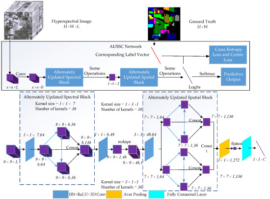
In this section, an alternately updated spectral–spatial convolutional network is proposed for HSI classification. Figure 1 shows an overview of the proposed method. For HSI data with L channels and a size of H × W , a spatial size of s × s was selected from the raw HSI data and used as the input to the AUSSC network. First, the AUSSC uses three smaller convolutional kernels to learn spectral and spatial features from an original HSI patch. Second, the alternately updated spectral and spatial blocks refine the deep spectral and spatial features using recurrent feedback. Finally, the model parameters are optimized using the cross-entropy loss and center-loss loss functions. Details of each stage are elaborated in the following subsections.

2.1. Learning Spectral and Spatial Features with Smaller Convolutional Kernels

During HSI classification, deep CNN-based methods typically utilize preprocessing technology such as PCA. This is often followed by several convolutional layers with multiple activation functions and a classifier for obtaining classification maps. The convolution and activation can be formulated as
X i l + 1 = f ( j = 1 N X j l k j i l + 1 + b i l + 1 ) ,
where X j l is the i th input feature map for the ( l + 1 ) th layer, N is the number of feature maps in the ( l + 1 ) th layer, * is the convolution operation, f ( ) is an activation function, and k j i l + 1 and b i l + 1 are learnable parameters that can be fine-tuned using the back-propagation (BP) algorithm.
The 3D CNN, SSRN, and FDSSC algorithms all demonstrate that an end-to-end 3D-CNN-based framework outperforms 2D-CNN-based methods that include preprocessing or post-processing, as well as other deep learning-based methods. One reason for this is that an end-to-end framework can reduce pre-processing and subsequent post-processing, allowing the connection between the original input and the final output to be as close as possible. The model then includes more space that can be adjusted automatically by the data, thereby increasing the degree of fitness. Additionally, when applied to HSIs with a 3D structure, 1D convolution operations focus on spectral features. 2D convolution operations focus on spatial features and 3D convolution operations can learn both spatial and spectral features. However, 3D kernel parameters are larger than 2D or 1D kernel parameters when the number of convolutional layers and kernels is the same. As such, a large number of model parameters can lead to overfitting.
As such, we propose an end-to-end CNN-based framework that uses smaller convolutional kernels compared to other CNN-based methods. As shown in Figure 2, the AUSSC utilizes kernels for HSI classification, ignoring other specific architectures. The 3D CNN method uses two similar convolutional kernels with sizes of a × a × m 1 and a × a × m 2 , with the two convolutional kernels differing only in spectral dimension. SSRN uses a spectral kernel with a size of 1 × 1 × m and a spatial kernel with a size of a × a × d to learn spectral and spatial representations, respectively. Convolutional kernels dictate model parameters and determine which features are learned by the CNN. In contrast, we introduce the idea of factorization into smaller convolutions from InceptionV3 [26]. In this process, a larger 3D convolutional kernel with a size of a × a × m was divided into three smaller convolutional kernels with sizes of 1 × 1 × m , 1 × a × 1 , and a × 1 × 1 . This substantially reduced the number of parameters, accelerated the operation, and reduced the possibility of overfitting. As shown in Table 1, in the absence of bias (with all other conditions remaining the same), the convolutional kernel with a size of a × a × m included a 2 m parameters. The smallest convolutional kernel only included parameters, which is more economical than the other two. This increased the nonlinear representation capabilities of the model due to the use of multiple nonlinear activation functions.

2.2. Refining Spectral and Spatial Features via Alternately Updated Blocks

Deep CNN architectures have been used for HSI classification and have produced competitive classification results [17]. However, the connection structure in the convolutional layers is typically in the forward direction. Additionally, the convolutional kernels in SSRN and FDSSC increase with depth. Alternately updated cliques have a recurrent feedback structure and go deeper into the convolutional layers with a fixed number of parameters [25]. Therefore, we propose combining small convolutional kernels with this loop structure and design two alternately updated blocks to learn refined spectral and spatial features separately from HSIs.
As shown in Figure 3, there are two stages in the alternately updated spectral blocks. In the initialization stage (stage 1), the 3D convolutional layers use k kernels with sizes of 1 × 1 × m to learn deep spectral features. In stage 2, the 3D convolutional layers use k kernels with sizes of 1 × 1 × m to learn refined spectral features. A feature map with a size of s × s × b and a number, n , was input to the alternately updated spectral block. This input is denoted as X 0 ( 1 ) , where the subscript 0 represents the feature map in the initial position of the alternately updated spectral block. The superscript (1) indicates the feature map is in the first stage of the alternately updated process. In stage 1, the input of every convolutional layer is the output of all the previous convolutional layers. Stage 1 can be formulated as follows:
X l ( 1 ) = f ( j < l X j ( 1 ) W j l ) ,
where X l ( 1 ) is the output of the lth ( l 1 ) convolutional layer in stage 1 of an alternately updated spectral block, f ( · ) is a nonlinear activation function, is the convolutional operation using the padding method, and W W j l is a parameter reused in stage 2.
In the looping stage (stage 2), each convolutional layer (except the input convolutional layer) is alternately updated to refine features. Stage 2 has a recurrent feedback structure, meaning that the feature map can be refined several times using the same weights. Therefore, any two convolutional layers in the alternately updated spectral block are connected bi-directionally. Stage 2 can then be formulated as follows:
X l r = f ( j < l X j r W j l + k > l X k ( r 1 ) W k l ) ,
where r 2 since the feature map is in stage 2 and can be updated multiple times by the recurrent feedback structure. Similarly, l 1 since the input feature map is not updated.
After learning refined deep spectral features, the input convolutional layer and the updated convolutional layer are concatenated in the alternately updated spectral block and transferred to the next block. Once spectral information from the HSI has been learned, the high dimensions of the feature map can be reduced by valid convolution and reshaping operations (see figure in Section 2.4.). The resulting input to the alternately updated spatial block is a feature map with number, n , and size t × t × 1 .
As shown in Figure 4, there are two different convolutional kernels in the alternately updated spatial block. The 3D convolutional layers use k a × 1 × 1 and k 1 × a × 1 convolutional kernels to learn deep refined spatial features with an alternately updated structure that is also used for the alternately updated spectral block. In the spatial block, two different convolutional kernels learn spatial features in parallel rather than in series. The convolutional relationship between the spatial block is the same as for the previous block.
These alternately updated blocks achieve spectral and spatial attention due to the presence of refined features obtained in the looping stages. Densely connected forward and feedback structures allow the spectral and spatial information to flow in convolutional layers within the blocks. These alternately updated blocks also include weight sharing. In stage 1, the weights increase linearly as the number of convolutional layers increases. However, in stage 2, the weights are fixed since they are shared. The partial weights from stage 1, such as W 12 , W 13 , and W 23 (see Figure 2), are reused in stage 2. As features are cycled repeatedly in stage 2, the number of parameters remains unchanged.

2.3. Optimization by the Cross-Entropy Loss and Center Loss Functions

HSI classification is inherently a multi-classification task and cross-entropy loss with a softmax layer is a well-known objective function that is used for such problems. The softmax cross-entropy loss can be written in the following form:
s o f t max = i = 1 m log exp ( W y i T x i + b y i ) j = 1 n exp ( W j T x i + b j ) ,
where m is the size of the mini-batch, n is the number of classes, x i is the i th deep feature belonging to the y i th class, W j is the j th column of the weights W in the last fully connected layer, and b is the bias. The last layer of the CNN-based model is typically fully connected, as it is difficult to make the dimensions of the last layer equal to the number of categories without a fully connected layer. Intuitively, one would expect that learning more discriminatory features would improve the generalization performance. As such, we introduce an auxiliary loss function [24] to improve the discrimination of features acquired by the model. This function can be formulated as follows:
c e n t e r = 1 2 i = 1 m x i c y i 2 2 ,
where c y i is the central feature in the y i th class. The function decreases the quadratic sum of the distance from the center of the feature to the features of each sample in one batch, which decreases the intra-class distance. The center of feature c y i can then be updated through iterative training.
When two loss functions are used together for HSI classification, the softmax cross-entropy loss is considered to be responsible for increasing the inter-class distance. The center loss is then responsible for reducing the intra-class distance, thus increasing the discriminant degree and generalization abilities of learned features. Consequently, the objective function for the AUSSC can be written in the following form:
= soft max + λ c e n t e r = i = 1 m log exp ( W y i T x i + b y i ) j = 1 n exp ( W j T x i + b j ) + λ 2 i = 1 m x i c y i 2 2
where λ ∈ [0, 1) controls the proportion of center loss and the value of λ is determined experimentally, as discussed in the following section. In summary, the cross-entropy loss is the principal objective function and the inter-class distance is the principal component. The center loss is the auxiliary used to reduce the intra-class distance.

2.4. Alternatively Updated Spectral–Spatial Convolutional Network

A flowchart is included below to explain the steps in the AUSSC end-to-end network. Considering the cost and time requirements of the collection of HSI labeled samples, we propose a 3D CNN-based framework that maximizes the flow and circulation of spectral and spatial information. Figure 5 shows a 9 × 9 × L cube, which is used as input in our technique, where L is the number of HSI bands. Due to high computational costs, two convolutional layers were used in the alternately updated blocks and a single loop was used in stage 2.
L2 loss and batch normalization (BN) [27] were used to improve the normalization of our model. In a broad sense, L2 and other regularization parameter terms added to the loss function in machine learning are essentially weighted norms. The goal of normalization with L2 loss is to effectively reduce the size of the original parameter values in the model, with BN performing normalization operations on input neuron values. The normalization target regularizes its input value to a normal distribution with a mean value of zero and a variance of one. The blue layers and blue lines both refer to the BN, rectified linear units (ReLU), and the convolution operation. The first convolutional layer lacks both a BN and a ReLU.
The original HSI input, which has a size of 9 × 9 × L , flows to the first convolutional layer with a kernel size of ( 1 , 1 , 7 ) and a stride of ( 1 , 1 , 2 ) to generate feature maps with a size of 6   49 × 9 × b . The number of kernels in the convolutional layers of alternately updated spectral block was 36, the kernel size was ( 1 , 1 , 7 ) , and the convolutional padding method was the same. As a result, the output size for each layer remained 36   9 × 9 × b , which was unchanged in stage 1 and stage 2. After concatenating the input and updated feature maps, the output of the alternately updated spectral blocks had a size of 136   9 × 9 × b .
A valid convolutional layer with 48 channels and a kernel size of 1 × 1 × b was included between alternately updated spectral and spatial blocks. This reduced the dimensions of the output of alternately updated spectral blocks, resulting in 48 feature maps with a size of 9 × 9 × 1. After reshaping the third dimension and the channel dimension, 48 channels with a size of 9 × 9 × 1 were merged into a single 9 × 9 × 48 channel. A valid convolutional layer with a kernel size of 3 × 3 × 48 and 64 kernels transformed the feature map into 64 channels with a size of 7 × 7 × 1 .
Similar to the alternately updated spectral blocks, the alternately updated spatial block featured two convolutional kernels with sizes of 1 × 3 × 1 and 3 × 1 × 1 . In stage 1 and stage 2, the output of each layer was 36 kernels with a size of 7 × 7 × 1. The results of two convolutional kernels were concatenated into 272 kernels with a size of 7 × 7 × 1. Finally, the output passed through a 3D average pooling layer with a pooling size of 7 × 7 × 1 , which was converted into 272 feature maps with a size of 1 × 1 × 1. After the flattening operation, a vector with a size of 1 × 1 × C was produced by the fully connected layer, where C is the number of classes. Trainable AUSSC parameters were optimized by iterative training using Equation (6) and used to compute the loss between the predicted and real values.
The following sections provide a summary of the advantages of this proposed AUSSC architecture. First, the use of three different small convolutional kernels reduced both the number of parameters and overfitting, thereby increasing the nonlinear representation ability of the model and the diversity of features. Compared with symmetric splitting into several identical small convolutional kernels, this asymmetric splitting can handle more and richer features. Second, refined deep features learned by both forward and feedback connections between convolutional layers are more robust and have more high-level spectral and spatial information. Additionally, SSRN and FDSSC learn deeper features by increasing the number of convolutional layers in the blocks. However, unlike these conventional models, AUSSC can go deeper with fixed parameters due to its loop structure and shared weights. Finally, an auxiliary loss function was used to reduce the intra-class distance and increase the distinction between features of different categories.

3. Experimental Data Sets and Framework Settings

3.1. Description of Experimental Data Sets

Three common HSI data sets were used to validate the proposed AUSSC, as follows: The Indiana Pines (IP; northwestern Indiana, USA), Kennedy Space Center (KSC; Merritt Island, FL, USA), and Salinas Scene (SS; Salinas Valley, CA, USA). These IP data were obtained by the NASA Airborne Visible Imaging Spectrometer (AVIRIS) sensor. The size of the IP data was 145 × 145 , with 220 bands containing 16 kinds of ground cover. The KSC data were collected by the AVIRIS sensor in 1996 and had a size of 512 × 614 , with 176 bands and 13 ground truth classes. The SS data were also collected by the AVIRIS sensor and had a size of 512 × 217 , with 204 bands and 9 ground truth classes. Table 2 lists these classes and the corresponding false-color composite maps for three data sets.
However, with the development of state-of-art algorithms for hyperspectral image classification, these three data sets are easily classified. When the number of training samples was more than 800, SSRN and FDSSC achieved an accuracy higher than 98% for the three HSI data sets. The difference between the classification accuracies of these methods is less than 1%. Therefore, in addition to the three data sets discussed above, this study included the Houston (Houston, TX, USA) data set, which was distributed for the 2013 GRSS Data Fusion Contest [28]. The Houston data are more difficult as conventional algorithms (SSRN, FDSSC, etc.) have been unable to achieve classification above 90% with 200 labeled training samples. The size of the Houston data was 349 × 1905 , with 144 bands containing 15 kinds of ground cover. Table 3 lists the classes and corresponding false-color composite maps for this data set.
Quantitative analysis was performed with the same limited training samples using all methods. Different sets of training samples were used to demonstrate the effectiveness of the AUSSC method under different conditions. A subset of 200 labeled samples were used for training and 100 labeled samples were used for validating. A series of 400, 600, 800, and 1000 training samples were then included to test the robustness and generalizability of the proposed AUSSC.

3.2. Framework Setting

The framework for all data sets was established as follows. From 10 random seeds, all data sets were randomly divided into the three following groups: A training set, a validation set, and a test set. The training sets were used to optimize model parameters. The validation sets were not directly used in the training process and were only included to verify whether the model was overfitting. The testing sets were used to test the performance of the model after the training was completed. The number of validation sets was half the number of training sets and the remainder of the sets were test sets. The batch size was set to 16 and the Adam [29] optimizer was used for stochastic optimization. The initialization of model weights was performed using the He normal distribution method [30] for all 3D convolutional layers and the Xavier normal distribution method for the fully connected layer [31]. We used a variable learning rate, which was gradually reduced during the optimization process. This was done because the learning rate must be smaller when closer to the valley. The number of training epochs was set to 400 and the initial learning rate was set to 0.0001 for IP, KSC, and SS data sets and 0.0003 for the Houston data set. The learning rate was halved when the validation loss did not decrease after 10 epochs.
In addition to these basic settings, four key factors were used to configure the AUSSC framework for HSI classification. Namely, (1) the number of convolutional layers and loops in one block of stage 2; (2) the number of convolutional kernels in alternately updated blocks; (3) the spatial size of input cubes; and (4) the coefficients of the center loss function. These four factors are discussed by the OA of IP, KSC, and SS below.
First, the number of convolutional layers and loops in each block of stage 2 determined the depth of the entire network, which consequently affected classification accuracy and runtime. As shown in Figure 6, appropriately increasing the number of convolutional layers and the number of loops improved classification. However, the network depth had a significant impact on training time and was almost linearly related to the training time. Therefore, we used two convolutional layers and only loop in each block to conserve training time.
Second, increasing the number of convolutional kernels often extracted more rich features. If enough convolutional kernels were provided, abstract high-order structures could be efficiently learned from the convolutional layer. As shown in Figure 7, the overall accuracy (OA) of the AUSSC was weakly positively related to the number of convolutional kernels, which had little effect on training time. Combining the performance of the AUSSC for the three data sets, the number of kernels in the first convolutional layer was set to 64 in each block and the number of kernels was set to 36 in two blocks.
Third, a larger input space allowed more spatial information to be extracted. Input samples with spatial sizes of 5 × 5 , 7 × 7 , 9 × 9 , and 11 × 11 were used in the three data sets. As shown in Figure 8, the OAs of the IP, KSC, and SS data sets increased with increasing input spatial size. However, for inputs with spatial sizes greater than or equal to 9 × 9, the increase in OA was less than 1%. Considering the cost of calculation, the 9 × 9 spatial size was selected for all data sets to test the performance of the AUSSC framework.
Moreover, the coefficient of center loss also played an important role in our proposed AUSSC. The coefficient of L2 loss was set to 0.0001 and the possible values of the coefficients for center loss were set to 0, 0.1, 0.01, and 0.001. As shown in Figure 9, the center loss could not be used directly as an objective function. However, as an auxiliary objective function, the center loss can slightly increase the overall classification accuracy. When the coefficient of center loss was set to 0.001, the OA of the AUSSC using the IP and SS data sets increased slightly. However, the OA of the AUSSC using the KSC data set increased by nearly 1%. As such, the coefficient of center loss was set to 0.001.

4. Classification Results and Discussion

4.1. Experimental Results

In this section, we compare the proposed AUSSC framework with deep learning-based methods, including SAE-LR [14], CNN [18], SSRN [21], 3D-GAN [24], and FDSSC [22]. As SSRN, FDSSC, and the proposed AUSSC are all 3D CNN-based methods, the input spatial size was fixed at 9 × 9 to allow a fair comparison. Ten groups of 200 training samples were randomly selected from the IP, KSC, SS, and Houston data sets. The classification accuracy indices for the experiment included the OA, average accuracy (AA), and kappa coefficient (Κ). The results of these three metrics are displayed in the form of mean ± standard deviation. The original hyperspectral data were normalized to a zero mean and standard deviation of one. The dimensions of the image block were the same as those of the original hyperspectral data. Figure 10, Figure 11, Figure 12 and Figure 13 show classification results obtained from the IP, KSC, SS, and Houston data sets using different algorithms.
Table 4, Table 5, Table 6 and Table 7 display the results of the OA, AA, kappa coefficient, and accuracy of each category for the IP, KSC, SS, and Houston data sets and the best accuracy is shown in bold. These experimental results show that our proposed AUSSC method is superior to early deep learning methods (SAE-LR and CNN), novel 3D-GAN, and recent 3D CNN-based methods (SSRN and FDSSC).
As shown in Table 4, the values of OA, AA, and K, obtained using the AUSSC, were 2.43%, 11.28%, and 2.75% higher than those obtained using FDSSC, which exhibited the second-best performance for the IP data set. AUSSC also achieved the best classification accuracy in 10 categories of the IP data set. AUSSC achieved an accuracy similar to SSRN and 3D-GAN for Class 4 (Corn) and Class 8 (Hay-windrowed), respectively. FDSSC achieved significantly better results for Class 11 (Soybean-mintill) and Class 13 (Wheat). However, FDSSC (like other methods), achieved poor results for Class 9 (Oats), with an average accuracy of only 10%. In contrast, AUSSC achieved excellent results with an average accuracy of 92.61%. CNN achieved the best results for Class 16 (Stone-Steel-Towers) but produced 0% for Class 9 (Oats) and performed poorly in four other categories.
As shown in Table 5, the values of OA, AA, and K obtained using AUSSC were respectively 1.37%, 3.34%, and 1.48% higher than those produced by 3D-GAN, which exhibited the second-best performance for the KSC data set. AUSSC also achieved the best accuracy in 7 of 13 KSC categories, producing results similar to those of 3D-GAN for Class 10 (Cattail marsh) and Class 11 (Salt marsh). 3D-GAN achieved significantly better results for Class 5 (Oak), Class 6 (Hardwood), and Class 7 (Swamp). However, its accuracy for Class 2 (Willow swamp) and Class 8 (Graminoid marsh) was ~20% lower than that of our method.
As shown in Table 6, the values of OA and K obtained using AUSSC were 0.63% and 0.71% higher than those produced by FDSSC, which exhibited the second-best performance for the SS data set. AUSSC achieved similar or better results than FDSSC across all 16 categories in the SS data set. As shown in Table 7, the values of OA, AA, and K, obtained using AUSSC, were 1.81%, 1.91%, and 1.95% higher than those obtained by FDSSC, which exhibited the second-best performance for the Houston data set. CNN achieved excellent results for Class 2 (Grass Stressed), Class 5 (Soil), and Class 15 (Running Track). However, the accuracy of CNN in Category 10 (Highway), Class 12 (Parking Lot 1), and Class 13 (Parking Lot 2) was ~40% lower than that of our method.
These experimental results indicate AUSSC achieved the best performance in terms of OA and K for all four HSI data sets. Other methods, especially CNN, were superior to our methods in some categories, but performed poorly in others. These poorly performing categories dramatically reduced the OA, AA, and K.
With the exception of the 3D-GAN data, which were obtained from the literature, these classification results shown in Table 4, Table 5, Table 6 and Table 7 were trained and tested using a desktop computer with 32 GB of memory equipped with an NVIDA GTX 1080Ti GPU. Table 8 shows the mean and standard deviation of the training time and testing time for 10 runs using CNN-based methods and the minimum time is shown in bold. As shown in the tables, the training times for deep 3D CNN-based methods were longer than those of other deep learning-based methods. The AUSSC required a longer training time than SSRN or FDSSC. For AUSSC applied to the IP data set, the number of floating-point operations per second (FLOPs) was 5362.386 K and the number of parameters was 761.064 K.
To corroborate the robustness and generalizability of the proposed method, Figure 14 and Figure 15 show the OA obtained using different methods for different training samples. When the number of training samples was higher than 400, our method performed similarly to SSRN and FDSSC. This is because the OA of SSRN and FDSSC reached more than 98%, creating a small gap between our method and these conventional techniques. This also demonstrates that the three datasets published more than 10 years ago are easily classified by state-of-the-art methods. The Houston data set, provided by the University of Houston for the 2013 IEEE GRSS Data Fusion Contest, is more challenging. As shown in Figure 15, it is more discriminant than the three datasets in comparing AUSSC with other methods. The resulting difference in OA between AUSSC, FDSSC, and SSRN was more than 1%.

4.2. Discussion

In this study, a highly limited number of training samples (200) was used to demonstrate that our proposed method can reduce data dependence. Insufficiently labeled data are unavoidable in remote sensing applications. Additionally, the collection and labeling of remote sensing data is complex and expensive. Thus, it is very difficult to build large-scale, high-quality labeled sets. The number of labeled samples used for training is the most important factor in deep-learning supervised methods, as data dependence is one of the most serious problems in deep learning. Compared with traditional machine-learning methods, deep learning relies heavily on large-scale training data, which are necessary to understand potential patterns. Semi-supervised 3D-GANs also require ~200 training samples; however, their classification accuracy is significantly lower.
The proposed method offers three principal benefits. First, it provides an end-to-end framework for HSI classification. SAE-LR, CNN, and 3D-GAN all require PCA to preprocess hyperspectral data. Second, deep CNN architectures and convolutional kernels were used to determine classification accuracy in 3D CNN-based methods [20]. These networks include only two convolutional layers with 3 × 3 × m convolutional kernels. SSRN and FDSSC use residual blocks, dense blocks, and two different convolutional kernels to learn deep spectral and spatial features. The biggest difference between AUSSC and the 3D CNN-based methods discussed above is its use of recurrent CNN architectures and three 1D convolutional kernels. Alternately updated blocks can not only learn deep spectral and spatial features but also refined spectral and spatial features. As a result, three 1D convolutional kernels can be combined to generate more abundant features. As a result, AUSSC achieved better classification accuracy than current state-of-the-art deep learning-based methods. Finally, unlike these other methods, only cross-entropy objective functions were used in the AUSSC. We also introduced center loss in the AUSSC as an auxiliary objective function to learn more discriminating features.
Although the proposed method provides better performance than conventional architectures (especially SSRN and FDSSC), it has a much higher computational requirement (see Table 8). There are three primary reasons for this. First, AUSSC uses more convolutional kernels in two blocks than SSRN and FDSSC. Second, the use of the center loss function increases the computational cost. Finally, and most importantly, more training epochs are used in AUSSC than in SSRN and FDSSC. In fact, the training time for one epoch in AUSSC is only slightly longer than in FDSSC or SSRN. However, AUSSC requires far more training epochs. The regular updating of graphics cards and the use of high performance graphics cards, such as the NVIDIA GeForce RTX 2080Ti, could effectively alleviate this problem.

5. Conclusions

In this study, refined spectral and spatial features in HSIs were used as core concepts to design an end-to-end CNN-based framework for HSI classification. This alternately updated convolutional spectral–spatial network utilizes alternately updated spectral and spatial blocks and primarily includes small convolutional kernels in three different dimensions to learn HIS features, combining them into advanced features.
The learning of deep refined spectral and spatial features by alternately updated blocks makes our method superior to other deep learning-based methods, as this allows it to achieve a high classification accuracy. Furthermore, experimental results also demonstrated that the center loss function can slightly improve the classification accuracy of hyperspectral images. Results showed that when 200 training samples were used from different HSI data sets, the AUSSC achieved the highest classification accuracy among the deep learning-based methods for all three data sets. Additionally, using different training samples, the AUSSC was also found to be the best method in terms of OA for all HSI data sets. However, the AUSSC has a longer training time than other conventional algorithms. In a future study, network pruning will be used to reduce the heavy calculation of the deep model.

Author Contributions

All authors made significant contributions to this work. W.W. and S.D. conceived and designed the experiments; S.D. performed the experiments; W.W. and S.W. analyzed the data; and S.W. contributed analysis tools.

Funding

The financial support for this work was provided in part by the Natural Science Foundation of Shanghai under Grant 19ZR1435900, in part by the Bidding Project of in part by the Bidding Project of the Lab of Green Plate-making and Standardization for Flexographic Printing under Grant ZBKT201710 and in part by the Shanghai Research Institute of Publishing and Media in 2018 under Grant SAYB1803.

Acknowledgments

The IP, KSC, and SS data used in this study were obtained from public domains and are available online at http://www.ehu.eus/ccwintco/index.php?title=Hyperspectral_Remote_Sensing_Scenes. The authors would like to thank the Hyperspectral Image Analysis group and the NSF Funded Center for Airborne Laser Mapping (NCALM) at the University of Houston for providing the Houston data set used in this study and the IEEE GRSS Data Fusion Technical Committee for organizing the 2013 Data Fusion Contest.

Conflicts of Interest

The authors declare no conflicts of interest. The funders had no role in the design of the study; in the collection, analysis, or interpretation of data; in the writing of the manuscript; nor in the decision to publish the results.

References

  1. Willett, R.M.; Duarte, M.F.; Davenport, M.A.; Baraniuk, R.G. Sparsity and structure in hyperspectral imaging: Sensing, reconstruction, and target detection. IEEE Signal Process. Mag. 2014, 31, 116–126. [Google Scholar] [CrossRef]
  2. Caporaso, N.; Whitworth, M.B.; Grebby, S.; Fisk, I.D. Non-destructive analysis of sucrose, caffeine and trigonelline on single green coffee beans by hyperspectral imaging. Food Res. Int. 2018, 106, 193–203. [Google Scholar] [CrossRef] [PubMed]
  3. Thomas, S.; Kuska, M.T.; Bohnenkamp, D.; Brugger, A.; Alisaac, E.; Wahabzada, M.; Behmann, J.; Mahlein, A.K. Benefits of hyperspectral imaging for plant disease detection and plant protection: A technical perspective. J. Plant Dis. Prot. 2018, 125, 5–20. [Google Scholar] [CrossRef]
  4. Lu, X.Q.; Yuan, Y.; Zheng, X.T. Joint dictionary learning for multispectral change detection. IEEE Trans. Cybern. 2017, 47, 884–897. [Google Scholar] [CrossRef] [PubMed]
  5. Lu, G.L.; Fei, B.W. Medical hyperspectral imaging: A review. J. Biomed. Opt. 2014, 19, 010901. [Google Scholar] [CrossRef] [PubMed]
  6. Melgani, F.; Bruzzone, L. Classification of hyperspectral remote sensing images with support vector machines. IEEE Trans. Geosci. Remote Sens. 2004, 42, 1778–1790. [Google Scholar] [CrossRef] [Green Version]
  7. Ghamisi, P.; Maggiori, E.; Li, S.; Souza, R.; Tarablaka, Y.; Moser, G.; Giorgi, A.D.; Fang, L.; Chen, Y.; Chi, M.; et al. New frontiers in spectral-spatial hyperspectral image classification: The latest advances based on mathematical morphology, markov random fields, segmentation, sparse representation, and deep learning. IEEE Geosci. Remote Sens. Mag. 2018, 6, 10–43. [Google Scholar] [CrossRef]
  8. Fauvel, M.; Benediktsson, J.A.; Chanussot, J.; Sveinsson, J.R. Spectral and spatial classification of hyperspectral data using svms and morphological profiles. IEEE Trans. Geosci. Remote Sens. 2008, 46, 3804–3814. [Google Scholar] [CrossRef]
  9. Ghamisi, P.; Benediktsson, J.A.; Ulfarsson, M.O. Spectral-spatial classification of hyperspectral images based on hidden markov random fields. IEEE Trans. Geosci. Remote Sens. 2014, 52, 2565–2574. [Google Scholar] [CrossRef]
  10. Chen, Y.; Nasrabadi, N.M.; Tran, T.D. Hyperspectral image classification via kernel sparse representation. IEEE Trans. Geosci. Remote Sens. 2013, 51, 217–231. [Google Scholar] [CrossRef]
  11. Chen, Y.; Lin, Z.; Zhao, X.; Wang, G.; Gu, Y. Deep learning-based classification of hyperspectral data. IEEE J. Sel. Top. Appl. Earth Obs. Remote Sens. 2014, 7, 2094–2107. [Google Scholar] [CrossRef]
  12. Zhang, L.; Zhang, L.; Du, B. Deep learning for remote sensing data: A technical tutorial on the state of the art. IEEE Geosci. Remote Sens. Mag. 2016, 4, 22–40. [Google Scholar] [CrossRef]
  13. Chen, Y.S.; Zhao, X.; Jia, X.P. Spectral-spatial classification of hyperspectral data based on deep belief network. IEEE J. Sel. Top. Appl. Earth Obs. Remote Sens. 2015, 8, 2381–2392. [Google Scholar] [CrossRef]
  14. Makantasis, K.; Karantzalos, K.; Doulamis, A.; Doulamis, N. Deep supervised learning for hyperspectral data classification through convolutional neural networks. In Proceedings of the 2015 IEEE International Geoscience and Remote Sensing Symposium, New York, NY, USA, 26–31 July 2015; pp. 4959–4962. [Google Scholar]
  15. Chen, Y.; Jiang, H.; Li, C.; Jia, X.; Ghamisi, P. Deep feature extraction and classification of hyperspectral images based on convolutional neural networks. IEEE Trans. Geosci. Remote Sens. 2016, 54, 6232–6251. [Google Scholar] [CrossRef]
  16. Li, Y.; Zhang, H.; Shen, Q. Spectral-spatial classification of hyperspectral imagery with 3d convolutional neural network. Remote Sens. 2017, 9, 67. [Google Scholar] [CrossRef]
  17. Zhong, Z.L.; Li, J.; Luo, Z.M.; Chapman, M. Spectral-spatial residual network for hyperspectral image classification: A 3-d deep learning framework. IEEE Trans. Geosci. Remote Sens. 2018, 56, 847–858. [Google Scholar] [CrossRef]
  18. Wang, W.J.; Dou, S.G.; Jiang, Z.M.; Sun, L.J. A fast dense spectral-spatial convolution network framework for hyperspectral images classification. Remote Sens. 2018, 10, 1068. [Google Scholar] [CrossRef]
  19. Ma, X.; Wang, H.; Wang, J. Semisupervised classification for hyperspectral image based on multi-decision labeling and deep feature learning. ISPRS J. Photogramm. Remote Sens. 2016, 120, 99–107. [Google Scholar] [CrossRef]
  20. Zhu, L.; Chen, Y.S.; Ghamisi, P.; Benediktsson, J.A. Generative adversarial networks for hyperspectral image classification. IEEE Trans. Geosci. Remote Sens. 2018, 56, 5046–5063. [Google Scholar] [CrossRef]
  21. Mnih, V.; Heess, N.; Graves, A.; Kavukcuoglu, K. Recurrent models of visual attention. In Proceedings of the 28th Annual Conference on Neural Information Processing Systems, Montreal, QC, Canada, 8–13 December 2014; pp. 2204–2212. [Google Scholar]
  22. Wang, F.; Jiang, M.; Qian, C.; Yang, S.; Li, C.; Zhang, H.; Wang, X.; Tang, X. Residual attention network for image classification. In Proceedings of the 30th IEEE Conference on Computer Vision and Pattern Recognition, CVPR, Honolulu, HI, USA, 21–26 July 2017; pp. 6450–6458. [Google Scholar]
  23. Stollenga, M.F.; Masci, J.; Gomez, F.; Schmidhuber, J. Deep networks with internal selective attention through feedback connections. In Proceedings of the 28th Annual Conference on Neural Information Processing Systems, Montreal, QC, Canada, 8–13 December 2014; pp. 3545–3553. [Google Scholar]
  24. Wen, Y.; Zhang, K.; Li, Z.; Qiao, Y. A discriminative feature learning approach for deep face recognition. In Computer Vision–Eccv 2016: 14th European Conference, Amsterdam, the Netherlands, October 11–14, 2016, Proceedings, Part VII; Leibe, B., Matas, J., Sebe, N., Welling, M., Eds.; Springer International Publishing: Cham, Switzerland, 2016; pp. 499–515. [Google Scholar]
  25. Yang, Y.B.; Zhong, Z.S.; Shen, T.C.; Lin, Z.C. Convolutional neural networks with alternately updated clique. In Proceedings of the 2018 IEEE/Cvf Conference on Computer Vision and Pattern Recognition, Salt Lake City, UT, USA, 18–23 June 2018; pp. 2413–2422. [Google Scholar]
  26. Szegedy, C.; Vanhoucke, V.; Ioffe, S.; Shlens, J.; Wojna, Z. Rethinking the inception architecture for computer vision. In Proceedings of the 2016 IEEE Conference on Computer Vision and Pattern Recognition, Las Vegas, NV, USA, 1 July 2016; pp. 2818–2826. [Google Scholar]
  27. Ioffe, S.; Szegedy, C. Batch normalization: Accelerating deep network training by reducing internal covariate shift. In Proceedings of the 32nd International Conference on Machine Learning, Lile, France, 6–11 July 2015; pp. 448–456. [Google Scholar]
  28. Debes, C.; Merentitis, A.; Heremans, R.; Hahn, J.; Frangiadakis, N.; van Kasteren, T.; Liao, W.Z.; Bellens, R.; Pizurica, A.; Gautama, S.; et al. Hyperspectral and lidar data fusion: Outcome of the 2013 grss data fusion contest. IEEE J. Sel. Top. Appl. Earth Obs. Remote Sens. 2014, 7, 2405–2418. [Google Scholar] [CrossRef]
  29. Kingma, D.P.; Ba, J.L. Adam: A method for stochastic optimization. In Proceedings of the International Conference on Learning Representations, San Diego, CA, USA, 7–9 May 2015; pp. 1–13. [Google Scholar]
  30. He, K.; Zhang, X.; Ren, S.; Sun, J. Delving deep into rectifiers: Surpassing human-level performance on imagenet classification. In Proceedings of the 15th IEEE International Conference on Computer Vision, Santiago, Chile, 11–18 December 2015; pp. 1026–1034. [Google Scholar]
  31. Glorot, X.; Bengio, Y. Understanding the difficulty of training deep feedforward neural networks. In Proceedings of the 13th International Conference on Artificial Intelligence and Statistics, Sardinia, Italy, 13–15 May 2010; pp. 249–256. [Google Scholar]
Figure 1. An overview of the proposed end-to-end alternately updated spectral–spatial convolutional network (AUSSC). “Conv” refers to the convolution operation. The operations denoted by “Some operations” are presented in detail in Section 2.4. “Logits” refers to the output of the last fully connected layer. Classification results are acquired after the Softmax operation.
Remotesensing 11 01794 g001
Figure 2. The structure of convolutional kernels in the 3D CNN-based method without a specific architecture. (a) 3D-CNN; (b) SSRN; (c) The proposed method. “Concat” refers to the concatenate operation.
Remotesensing 11 01794 g002
Figure 3. Two stages of alternately updated spectral blocks with three convolutional layers.
Remotesensing 11 01794 g003
Figure 4. A representation of the alternately updated spatial block with two different convolutional kernels and three convolutional layers for each convolutional kernel.
Remotesensing 11 01794 g004
Figure 5. The AUSSC proposed for hyperspectral image (HSI) classification of labeled pixels with an input size of 9 × 9 × L . The value L is the number of HSI bands and C is the number of classes.
Remotesensing 11 01794 g005
Figure 6. The overall accuracy of the AUSSC with different numbers of convolutional layers and loops in each block. The a + b notation on the x-axis denotes the AUSSC with a convolutional layers and b looping iterations in stage 2 of each block. IP: Indiana Pines data set; KSC: Kennedy Space Center data set; SS: Salinas Scene data set.
Remotesensing 11 01794 g006
Figure 7. The overall accuracy of the AUSSC with different numbers of convolutional kernels in the first layer using two blocks. The a + b notation on the x-axis denotes an AUCN with a kernels in the first convolutional layer and b kernels in the two blocks.
Remotesensing 11 01794 g007
Figure 8. The overall accuracy of the AUSSC with different input spatial sizes.
Remotesensing 11 01794 g008
Figure 9. The overall accuracy of AUSSC for different center-loss coefficients.
Remotesensing 11 01794 g009
Figure 10. Classification results for the Indian Pines data set obtained using different methods. (a) Ground-truth map; (b) SAE-LR; (c) CNN; (d) SSRN; (e) FDSSC; and (f) AUSSC.
Remotesensing 11 01794 g010
Figure 11. Classification results obtained from the KSC data set using different methods. (a) Ground-truth map; (b) SAE-LR; (c) CNN; (d) SSRN; (e) FDSSC; and (f) AUSSC.
Remotesensing 11 01794 g011
Figure 12. Classification results obtained from the SS data set using different methods. (a) Ground-truth map; (b) SAE-LR; (c) CNN; (d) SSRN; (e) FDSSC; and (f) AUSSC.
Remotesensing 11 01794 g012
Figure 13. Classification results obtained from the Houston data set using different methods. (a) Ground-truth map; (b) SAE-LR; (c) CNN; (d) SSRN; (e) FDSSC; and (f) AUSSC.
Remotesensing 11 01794 g013
Figure 14. The overall accuracy (OA) of different methods for different numbers of training samples in three HSI data sets. (a) Indiana Pines (IP) data set; (b) Kennedy Space Center (KSC) data set; and (c) Salinas Scene (SS) data set.
Remotesensing 11 01794 g014
Figure 15. The overall accuracy (OA) of different methods for different numbers of training samples in the Houston data set.
Remotesensing 11 01794 g015
Table 1. Parameters for different convolutional kernels.
Convolutional KernelsParameters
a × a × m a 2 m
1 × 1 × m a × a × 1 a 2 + m
1 × 1 × m a × 1 × 1 1 × a × 1 a + a + m
Table 2. Color codes for the classes, class types, and sample numbers (SN) for the ground truths of the Indiana Pines (IP) data, Kennedy Space Center (KSC) data, and Salinas Scene (SS) data.
ColorIP DataKSC DataSS Data
ClassSNClassSNClassSN
Remotesensing 11 01794 i001Alfalfa46Scrub347Brocoli_green_weeds_12009
Remotesensing 11 01794 i002Corn-notill1426Willow swamp243Brocoli_green_weeds_23726
Remotesensing 11 01794 i003Corn-mintill830CP hammock256Fallow1976
Remotesensing 11 01794 i004Corn237Slash pine252Fallow_rough_plow1394
Remotesensing 11 01794 i005Grass-pasture483Oak/Broadleaf161Fallow_smooth2678
Remotesensing 11 01794 i006Grass-trees730Hardwood229Stubble3959
Remotesensing 11 01794 i007Grass-pasture-mowed28Swamp105Celery3579
Remotesensing 11 01794 i008Hay-windrowed478Graminoid marsh390Grapes_untrained11271
Remotesensing 11 01794 i009Oats20Spartina marsh520Soil_vinyard_develop6203
Remotesensing 11 01794 i010Soybean-notill972Cattail marsh404Corn_senesced_green_weeds3278
Remotesensing 11 01794 i011Soybean-mintill2455Salt marsh419Lettuce_romaine_4wk1068
Remotesensing 11 01794 i012Soybean-clean593Mud flats503Lettuce_romaine_5wk1927
Remotesensing 11 01794 i013Wheat205Water927Lettuce_romaine_6wk916
Remotesensing 11 01794 i014Woods1265 Lettuce_romaine_7wk1070
Remotesensing 11 01794 i015Buildings-Grass-Trees386 Vinyard_untrained7268
Remotesensing 11 01794 i016Stone-Steel-Towers93 Vinyard_vertical_trellis1807
Total10,249521154,129
Table 3. Color codes for the classes, class types, and sample numbers (SN) for the ground truth of the Houston data.
NO.ColorClassSN
1 Remotesensing 11 01794 i001Grass Healthy1374
2 Remotesensing 11 01794 i002Grass Stressed1454
3 Remotesensing 11 01794 i003Grass Synthetic795
4 Remotesensing 11 01794 i004Tree1264
5 Remotesensing 11 01794 i005Soil1298
6 Remotesensing 11 01794 i006Water339
7 Remotesensing 11 01794 i007Residential1476
8 Remotesensing 11 01794 i008Commercial1354
9 Remotesensing 11 01794 i009Road1554
10 Remotesensing 11 01794 i010Highway1424
11 Remotesensing 11 01794 i011Railway1332
12 Remotesensing 11 01794 i012Parking Lot 11429
13 Remotesensing 11 01794 i013Parking Lot 2632
14 Remotesensing 11 01794 i014Tennis Court513
15 Remotesensing 11 01794 i015Running Track798
Total17,036
Table 4. Overall accuracy (OA), average accuracy (AA), kappa coefficient (K), and accuracy for each HSI category in the Indiana Pines (IP) data set. Data are given as mean ± standard deviation.
MethodsSAE-LRCNNSSRN3D-GANFDSSCAUSSC
OA (%)57.44   ±   0.5659.84   ±   0.9890.47   ±   2.2490.69   ±   0.8692.12   ±   1.0594.55   ±   1.09
AA (%)46.30   ±   1.1751.60   ±   1.1788.46   ±   3.2983.14   ±   1.8283.16   ±   5.0894.44   ±   1.11
Κ   × 100 51.04   ±   0.5853.97   ±   1.0389.12   ±   2.5489.62   ±   0.2691.02   ±   1.1893.77   ±   1.25
122.89   ±   7.331.33   ±   1.09 90.00   ±   30.030.21   ±   1.0370.00   ±   45.898.33   ±   5.00
245.46   ±   3.8041.53   ±   3.0487.35   ±   11.681.79   ±   0.2690.38   ±   4.8794.60   ±   3.04
326.69   ±   2.6130.91   ±   8.2887.18   ±   7.2475.93   ±   1.26 86.48   ±   3.9990.06   ±   4.53
433.80   ±   10.213.28   ±   4.1694.28   ±   6.6390.08   ±   1.2392.34   ±   6.6793.73   ±   5.98
546.82   ±   7.7870.80   ±   1.5995.89   ±   3.6686.39   ±   2.1296.65   ±   1.9598.59   ±   2.55
679.64   ±   1.7190.78   ±   0.7894.09   ±   2.0793.28   ±   0.23 95.11   ±   2.4497.84   ±   0.81
741.45   ±   10.520.74   ±   8.9571.98   ±   37.840.71   ±   1.0540.00   ±   49.086.57   ±   13.0
896.57   ±   1.2694.93   ±   4.0494.13   ±   3.3098.11   ±   0.2192.51   ±   2.0697.22   ±   2.11
938.82   ±   23.40.00   ±   0.0050.0   ±   50.020.00   ±   1.9610.00   ±   30.091.61   ±   9.49
1050.47   ±   1.9152.53   ±   1.2486.47   ±   7.6974.28   ±   0.8984.87   ±   9.3992.40   ±   2.86
1170.89   ±   2.4961.88   ±   4.3391.88   ±   5.0391.12   ±   0.2595.32   ±   2.1293.97   ±   3.29
1228.41   ±   6.6726.57   ±   2.9688.93   ±   6.2784.99   ±   1.4692.45   ±   4.3594.52   ±   2.55
1322.57   ±   8.2894.03   ±   1.3397.15   ±   4.1849.75   ±   2.4599.70   ±   0.9097.67   ±   2.99
1478.23   ±   5.8993.74   ±   1.4096.03   ±   3.1194.38   ±   0.26 96.39   ±   2.7496.65   ±   1.49
1539.57   ±   7.0833.46   ±   3.2392.00   ±   6.5094.47   ±   0.7990.36   ±   9.5594.63   ±   1.59
1618.59   ±   21.6 99.12   ±   0.8297.98   ±   2.7184.22   ±   1.1698.01   ±   1.3392.70   ±   5.28
Table 5. OA, AA, Κ, and accuracy for each HSI category in the Kennedy Space Center (KSC) data set.
MethodsSAE-LRCNNSSRN3D-GANFDSSCAUSSC
OA (%)57.68   ±   1.7469.87   ±   0.3696.23   ±   1.4096.89   ±   1.2496.28   ±   1.2698.26   ±   0.70
AA (%)44.99   ±   4.5969.59   ±   0.4494.58   ±   1.5394.14   ±   0.4094.58   ±   1.7097.48   ±   1.01
Κ   × 100 52.45   ±   1.9465.87   ±   0.3795.80   ±   1.5696.52   ±   0.2695.86   ±   1.4198.0   ±   0.78
181.87   ±   15.54.09   ±   2.7997.87   ±   3.5098.29   ±   0.4297.99   ±   2.2499.02   ±   1.02
252.83   ±   29.685.29   ±   1.9194.29   ±   5.6679.84   ±   1.4593.01   ±   4.3596.35   ±   6.83
335.82   ±   33.269.38   ±   1.9485.31   ±   13.798.44   ±   0.1486.65   ±   10.398.98   ±   3.05
40.00   ±   0.0032.06   ±   1.7884.11   ±   11.486.51   ±   1.1276.02   ±   10.787.54   ±   6.86
521.22   ±   22.452.50   ±   2.0982.92   ±   16.098.7   ±   0.1486.61   ±   11.294.24   ±   8.50
60.37   ±   0.5158.60   ±   1.4096.51   ±   5.23100.00   ±   0.0096.23   ±   5.8297.53   ±   4.94
723.56   ±   19.099.23   ±   1.5493.14   ±   8.0597.14   ±   1.0697.32   ±   4.6896.12   ±   8.69
866.24   ±   10.162.13   ±   2.4697.83   ±   1.6772.95   ±   2.1097.28   ±   2.2798.58   ±   0.87
951.76   ±   25.086.69   ±   0.3199.84   ±   0.2299.23   ±   0.0999.84   ±   0.1899.92   ±   0.13
1020.00   ±   14.473.47   ±   2.6799.02   ±   2.38100.00   ±   0.00100.00   ±   0.0099.97   ±   0.08
1189.64   ±   3.4890.00   ±   0.0099.50   ±   0.73100.00   ±   0.0098.70   ±   1.6399.18   ±   1.29
1251.24   ±   12.093.25   ±   0.4399.25   ±   0.8596.48   ±   1.2399.87   ±   0.2299.83   ±   0.25
1390.44   ±   3.0097.93   ±   0.2299.91   ±   0.21100.00   ±   0.00100.00   ±   0.00100.00   ±   0.00
Table 6. OA, AA, Κ, and accuracy for each HSI category in the Salinas Scene (SS) data set.
MethodsSAE-LRCNNSSRN3D-GANFDSSCAUSSC
OA (%)71.51   ±   0.1085.92   ±   2.7994.02   ±   2.7993.02   ±   1.5495.50   ±   0.6996.13   ±   0.57
AA (%)78.03   ±   0.1491.14   ±   2.0297.39   ±   0.6389.15   ±   0.3997.41   ±   0.3297.37   ±   0.53
Κ   × 100 68.48   ±   0.1184.42   ±   3.0393.34   ±   3.1092.07   ±   1.2294.99   ±   0.7795.70   ±   0.64
199.26   ±   0.26100.00   ±   0.00100.00   ±   0.0098.12   ±   1.02100.00   ±   0.00100   ±   0.00
298.90   ±   0.2299.42   ±   0.7798.90   ±   2.0094.11   ±   0.1299.82   ±   0.4299.82   ±   0.45
380.92   ±   0.8464.65   ±   20.898.38   ±   1.4076.46   ±   0.2895.40   ±   2.6095.04   ±   4.35
498.71   ±   0.1198.74   ±   0.3498.97   ±   0.94100.00   ±   0.4798.08   ±   1.5597.99   ±   1.47
574.30   ±   0.1997.69   ±   1.6398.92   ±   1.4688.25   ±   1.8999.42   ±   0.6198.69   ±   2.31
699.8   ±   0.0399.97   ±   0.0699.94   ±   0.1699.34   ±   0.3699.99   ±   0.0199.98   ±   0.05
799.22   ±   0.0999.74   ±   0.1799.97   ±   0.0199.90   ±   0.6799.44   ±   0.7999.56   ±   0.65
878.78   ±   3.1056.58   ±   19.789.97   ±   9.8689.44   ±   1.1390.27   ±   4.4292.83   ±   2.96
90.00   ±   0.0099.99   ±   0.0199.49   ±   0.66100.00   ±   0.0099.51   ±   0.4399.41   ±   0.21
1074.08   ±   0.8486.06   ±   4.3598.71   ±   1.7598.13   ±   1.0096.29   ±   3.2798.25   ±   2.22
1193.68   ±   0.2885.14   ±   4.3196.07   ±   2.0196.69   ±   2.1296.33   ±   1.5193.90   ±   4.29
1299.99   ±   0.0392.66   ±   8.3899.05   ±   0.6599.06   ±   1.0498.06   ±   1.7298.40   ±   1.60
1399.18   ±   0.0698.16   ±   3.0698.43   ±   1.8877.92   ±   1.6899.08   ±   1.2298.59   ±   1.41
1494.28   ±   0.4997.46   ±   1.8798.23   ±   1.6478.21   ±   0.6798.35   ±   1.6696.13   ±   4.98
1557.39   ±   0.9685.57   ±   8.7283.26   ±   11.870.88   ±   0.4588.62   ±   5.2189.32   ±   4.69
160.00   ±   0.0096.43   ±   5.90100.00   ±   0.0090.0   ±   0.1299.85   ±   0.3099.94   ±   1.70
Table 7. OA, AA, Κ, and accuracy for each HSI category in the Houston data set.
MethodsSAE-LRCNNSSRNFDSSCAUSSC
OA (%)76.18   ±   3.2275.01   ±   0.7588.89   ±   2.2589.40   ±   1.2691.21   ±   1.57
AA (%)75.44   ±   0.1476.45   ±   0.5891.35   ±   1.7191.39   ±   1.0293.30   ±   1.04
Κ   × 100 74.06   ±   3.8272.98   ±   0.8187.99   ±   2.4388.55   ±   1.3690.50   ±   1.70
195.96   ±   0.5486.61   ±   2.3891.44   ±   5.1990.91   ±   5.6696.17   ±   2.18
285.84   ±   0.1799.19   ±   0.1294.92   ±   3.0693.02   ±   8.5494.55   ±   3.26
395.35   ±   0.4195.42   ±   0.8199.50   ±   0.5599.49   ±   1.0399.61   ±   0.60
495.52   ±   0.1783.06   ±   1.0897.46   ±   2.8299.16   ±   0.3997.81   ±   2.37
594.28   ±   0.54100   ±   0.0096.55   ±   2.4096.61   ±   4.0897.84   ±   2.78
669.91   ±   1.2687.58   ±   0.2499.75   ±   0.74100   ±   0.00100   ±   0.00
770.46   ±   0.6470.69   ±   3.0883.18   ±   8.13 89.19   ±   3.0790.14   ±   7.56
868.31   ±   2.0562.17   ±   1.6996.18   ±   4.1095.81   ±   4.2395.89   ±   4.09
965.76   ±   0.1972.56   ±   4.6678.42   ±   6.49 83.22   ±   7.4878.91   ±   6.99
1059.64   ±   0.1949.79   ±   3.4578.51   ±   8.4079.95   ±   5.4887.78   ±   5.84
1176.71   ±   0.5676.32   ±   3.6282.14   ±   87.2382.99   ±   7.1289.28   ±   7.02
1288.03   ±   0.7936.12   ±   8.4188.03   ±   6.54 82.97   ±   6.5781.04   ±   8.89
1311.58   ±   0.4232.51   ±   5.4488.52   ±   8.2682.59   ±   8.2796.11   ±   0.40
1458.75   ±   0.3394.75   ±   1.3697.42   ±   3.6297.26   ±   3.1196.60   ±   3.25
1595.46   ±   0.57100   ±   0.0098.32   ±   0.8897.68   ±   1.5697.75   ±   1.46
Table 8. Training and testing times for CNN-based methods across the four data sets.
Data setTimeCNNSSRNFDSSCAUSSC
IPTraining/sec9.25   ±   0.4073.9   ±   5.3263.5   ±   3.72439   ±   4.16
Testing/sec0.71   ±   0.116.84   ±   0.207.91   ±   0.1111.1   ±   0.21
KSCTraining/sec8.10   ±   0.5172.0   ±   2.5057.1   ±   4.95420   ±   4.21
Testing/sec0.46   ±   0.162.18   ±   0.073.40   ±   0.064.83   ±   0.07
SSTraining/sec10.1   ±   0.5977.9   ±   3.0063.5   ±   4.02433   ±   3.99
Testing/sec2.05   ±   0.1127.0   ±   0.8643.1   ±   0.5058.9   ±   0.47
HoustonTraining/sec10.2   ±   0.55149   ±   4.3483. 5   ±   1.26594   ±   4.80
Testing/sec1.52   ±   0.0513.9   ±   0.4910.9   ±   0.1311.9   ±   0.18

