Abstract
The Southern Ocean (SO) is highly sensitive to climate change. Therefore, an accurate estimate of phytoplankton biomass is key to being able to predict the climate trajectory of the 21st century. In this study, MODerate resolution Imaging Spectroradiometer (MODIS), on board EOS Aqua spacecraft, Level 2 (nominal 1 km × 1 km resolution) chlorophyll-a (C) and Particulate Organic Carbon (POC) products are evaluated by comparison with an in situ dataset from 11 research cruises (2008–2017) to the SO, across multiple seasons, which includes measurements of POC and chlorophyll-a (C) from both High Performance Liquid Chromatography (C) and fluorometry (C). Contrary to a number of previous studies, results highlighted good performance of the algorithm in the SO when comparing estimations with HPLC measurements. Using a time window of ±12 h and a mean satellite chlorophyll from a 5 × 5 pixel box centered on the in situ location, the median C:C ratios were 0.89 (N = 46) and 0.49 (N = 73) for C and C respectively. Differences between C and C were associated with the presence of diatoms containing chlorophyll-c pigments, which induced an overestimation of chlorophyll-a when measured fluorometrically due to a potential overlap of the chlorophyll-a and chlorophyll-c emission spectra. An underestimation of ∼0.13 mg m was observed for the global POC algorithm. This error was likely due to an overestimate of in situ POC measurements from the impact of dissolved organic carbon not accounted for in the blank correction. These results highlight the important implications of different in situ methodologies when validating ocean colour products.
1. Introduction
The oceans play a substantial role in mediating global climate by sequestering 25–30% of anthropogenic CO from the atmosphere, with the Southern Ocean (SO) alone accounting for ∼40% of this total [1,2,3,4,5]. Biological production and carbon export to the deep ocean, “the biological pump” is considered a major contributor to the SO CO sink while also regulating the supply of nutrients (∼75%) to thermocline waters north of 30S, which in turn drives low latitude productivity [6]. Despite the ecological importance of this area, in situ data collection is often constrained through difficulties in accessing key areas by ship, primarily due to distance, weather and sea ice. This inability to resolve inter-annual variability and seasonal and intra-seasonal dynamics, limits our understanding of this complex system. Satellite remote sensing is one of the most effective tools available to address these spatial and temporal gaps in our knowledge. They have the added advantage of being routine, synoptic and available over decadal time scales and are in many cases, the only systematic observations available for chronically under-sampled marine systems such as the polar oceans. However, current ocean colour algorithms applied to SO data sets have been shown to perform badly, due proposedly to their typical parameterisation with low-latitude bio-optical data sets (in the absence of sufficient regional data) whose Inherent Optical Properties (IOPs) differ from those of the SO (e.g., [7]). Given the growing importance of the application of these tools in the trajectory of SO ecosystem understanding, it is necessary that we rigorously assess the quality of satellite-derived ocean colour data products such as chlorophyll-a (C) and particulate organic carbon (POC), which are currently used to study trends and trajectories of fundamental parameters such as phytoplankton biomass, primary production and the carbon cycle [8,9].
To the best of our knowledge, 20 previous studies have evaluated the ocean colour chlorophyll-a product in the SO, with most of these highlighting the poor performance of the algorithm with an average factor of 0.5 underestimate of retrieved chlorophyll-a relative to measured chlorophyll-a [7,10,11,12,13,14,15,16,17,18,19,20,21,22,23,24,25,26]. Holm-Hanssen et al. [18] highlighted variations in the bias associated with the range of chlorophyll-a concentration and found that in the Scotia Sea, where chlorophyll-a concentrations were <1 mg m, ratios of satellite retrieved to in situ chlorophyll-a concentration (C) were as high as 0.89 ± 0.45 (N = 50), whereas for chlorophyll-a concentrations between 1–4 mg m, lower ratios of 0.48 ± 0.18 (N = 30) were observed. Similarly, Clementson et al. [16] found a bias that depends on the concentration of chlorophyll-a with a tendency for the SeaWiFS OC4V4 algorithm to underestimate chlorophyll-a at high concentrations, while an overestimation was obtained when pigment concentrations were low (<0.15 mg m). Dierssen & Smith, ref. [14] hypothesised that the bias in retrieving accurate chlorophyll-a concentrations for the SO was attributed to lower concentrations of bacteria, which induce a lower backscattering coefficient for similar concentrations of chlorophyll-a. Another study by Reynolds et al. [15] similarly attributed poor algorithm performance to variability in the spectral backscattering ratio, which was deduced from differentiation in algorithm performance between the Ross Sea and the Antarctic Polar Front Zone (APFZ). The majority of studies however, refer to absorption as the primary IOP responsible for the failure of the application of global chlorophyll-a algorithms to the SO. These include the following: variations in the absorption coefficient of specific detritus and colored dissolved organic matter (CDOM) absorption relative to phytoplankton absorption, large pigment packaging of the dominant phytoplankton species due to low light adaptation, species composition, low chlorophyll-a specific absorption and species-specific absorption in the 440-570 nm range (e.g., [10,12,18,19,20,24,26,27]). To expand on one example, Dierssen, ref. [27] used the radiative transfer model Hydrolight to analyse the impact of variations in CDOM concentration, which typically vary in the blue part of the spectrum, as a function of geographical region, age and exposure to solar degradation processes. Using a range of CDOM concentrations at 440 nm from 0 to 0.03 m as model input, they were able to retrieve chlorophyll-a concentrations that ranged over a factor of 3 for oligotrophic waters (chlorophyll-a < 0.2 mg m). Worth noting is that most of the studies mentioned above used C measured from fluorometric methods rather than High Performance Liquid Chromatography (HPLC). In addition, many of the studies did not adhere to all the matchup procedures recommended by Bailey & Werdell, ref. [28] for their comparison between in situ and satellite data records. For instance, Johnson et al. [26] used daily, 8 days or monthly averaged NASA Aqua MODIS Level 3, 9 km data products.
On the contrary, two studies by Haëntjens et al. [29] and Marrari et al. [30] showed a good performance of global satellite algorithms in the SO over a large range of chlorophyll-a concentrations. Haëntjens et al. [29] compared chlorophyll−a and POC products of the Visible Infrared Imaging Radiometer Suite (VIIRS) on board Suomi-NPP spacecraft and the Aqua MODIS sensors with float measurements from the Southern Ocean Carbon and Climate Observations and Modeling (SOCCOM) programme. Here, chlorophyll-a and POC derived from fluorescence and backscattering sensors, were rigorously calibrated with samples collected at the time of the floats’ deployment. The authors conclude that the global algorithms perform well in the SO with an average agreement to within 9% and 12%, for VIIRS and Aqua MODIS respectively. Marrari et al. [30] on the other hand compared the SeaWIFS daily chlorophyll-a (resolution: ∼1 km/pixel) product (SeaDAS4.8, OC4v4 algorithm) with HPLC and fluorometric chlorophyll-a measurements collected during January–February of 1998–2002 around the Antarctic Peninsula. Their C/C ratio of 1.12 ± 0.91 (N = 96) showed good agreement, while the C/C ratio of 0.55 ± 0.63 (N = 307) suggested a ∼50% underestimation, which the authors attribute to low concentrations of chlorophyll-b and high concentrations of chlorophyll-c which impact the fluorescence measurements [27,30,31]. A more recent study by Pereira & Garcia, ref. [7] however, also in the northern Antarctic Peninsula observed an underestimation of the Aqua MODIS algorithm, regardless of the method used to estimate chlorophyll-a concentrations.
At this point, an evaluation of the performance of global ocean colour algorithms applied to the SO is inconclusive, highlighting the requirement for additional in situ data with large regional and seasonal coverage to support a rigorous assessment that adheres to strict matchup criteria [28]. The aim of this study is to evaluate Aqua MODIS Level 2 (nominal 1 km × 1 km resolution) chlorophyll-a and POC products using an in situ database (>1000 data points) of POC and chlorophyll-a measured from both HPLC and fluorometric methods, from 11 research cruises (2008–2017) to the SO, spanning multiple regions and seasons.
2. Material and Methods
2.1. In Situ Dataset
A database of fluorometric (N = 1527), HPLC (N = 1010) and POC (N = 1028) measurements were assimilated from 11 research cruises to the SO conducted between 2008 and 2017 (Table 1).

Table 1.
Southern Ocean research cruises during which POC, HPLC and fluorometric chlorophyll-a samples were collected.
Sample Collection and Storage
Surface seawater samples were collected from niskin bottles attached to a conductivity–temperature–depth (CTD) rosette system and an underway intake system (nominal depth ∼7 m). Fluorometric (0.25–0.5 L) and HPLC (0.5–2.0 L) samples were filtered onto GF/F filters (Whatman, diameter 25 mm, nominal pore size 0.7 m). Fluorometric samples were measured onboard the ship whilst HPLC samples were flash frozen in liquid nitrogen and stored at −80 C until analysis on land in Villefranche, France.
For fluorometric chlorophyll-a analysis, chlorophyll-a was extracted by placing the filters into 8 ml 90% acetone for 24 h in the dark at −20 C. Fluorometric chlorophyll-a was measured with a fluorometer (Turner Designs 10AUTM (SANAE 48) and Trilogy® (all other cruises) Laboratory Fluorometer) following Welschmeyer, [32]. Fluorescence chlorophyll was converted to chlorophyll-a using a standard chlorophyll-a dilution calibration. Samples for HPLC were extracted at −20 C in 3 mL of 100% Methanol, disrupted by sonication and then clarified by filtration and finally analysed on an Agilent Technologies HPLC 1200 following the methods of Ras et al. [33]. Note that total chlorophyll-c corresponds to the sum of chlorophyll-c1, c2 and c3, while total chlorophyll (C) corresponds to the sum of divinyl chlorophyll-a, monovinyl chlorophyll-a, chlorophyllide a, chlorophyll-a allomers, and chlorophyll-a epimers.
POC samples (0.5–2.0 L) were filtered through GF/F filters pre-combusted at 450 C. POC samples were dried in an oven at 40 C for 24 h before being acid fumed with concentrated HCl for 24 h to remove inorganic carbon. Filters were pelleted into 5 × 8 mm tin capsules and analysed with a Flash EA 1112 series elemental analyser (Thermo Finnigan). Dry blanks (pre combusted GF/F filters) were interspersed every 6 to 20 samples (typically every 12) and subtracted from each sample to obtain total POC (as per JGOFS POC protocols; [34]). On the most recent ACE cruise (Table 1), two additional filtered seawater (FSW) blanks were collected and analysed for POC content by filtering 2 L of seawater through a GF/F and then again through a pre-combusted GF/F, which was processed as above as an FSW-blank.
2.2. Satellite Data
Aqua MODIS Level 2 R2018.0 (nominal 1 km × 1 km resolution) data were acquired from the NASA Goddard Space Flight Center website [35]. The standard MODIS chlorophyll-a and POC products [36] (C and POC respectively) were evaluated by comparing in situ measurements with coincident satellite retrievals. A full description of the algorithm is provided in Appendix A. To ensure the quality of the matchup, an adjusted version of the Bailey & Werdell, ref. [28] procedure was applied (Figure 1). The time window to determine the closest coincidence between in situ and valid satellite data was 12 h instead of the 3 h initially advised by Bailey & Werdell, ref. [28], note however that the statistics for different time windows is presented in Table 2. Time averages were not performed, with only the closest matchup in time being recorded. For instance, for a time window of ±12 h, one matchup can be extracted at +3 h and another one at −6 h with a mean absolute time difference of 4.5 h. When a matchup was obtained, two pixel extractions were performed: a box of 5 by 5 pixels around the in situ location (named box 1), and, as recently proposed by Haëntjens et al. [29], all pixels in a radius of 8 km around the station (named box 2). Any pixel containing one or more of the following MODIS L2 quality flags ([37]) were excluded: suspect or failure in the atmospheric correction, land, sunglint, high radiance (near saturation), high sensor view zenith angle, shallow water pixels, stray light, cloud or ice contamination, coccolithophores, turbid water, high solar zenith angle, low water-leaving radiance, and moderate sun glint contamination. In addition, we masked all pixels with a solar zenith angle higher than 75 [28]. As the boxes contained several pixels, an analysis was performed to ensure the confidence of the mean value for each station. Only boxes containing >50% valid (unflagged) pixels were used for further analysis. In addition, only points within the mean ± 1.5 ×std (standard deviation) were considered. Finally, a test of homogeneity was performed by checking the coefficient of variation (CV), with the matchup being excluded if the CV was higher than 0.15 [28].
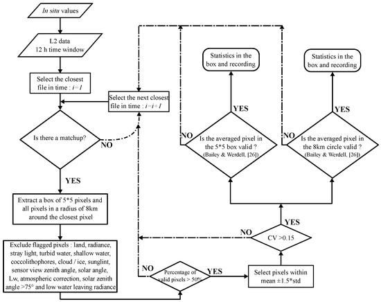
Figure 1.
Flowchart of the procedures applied to extract the satellite values.
Table 2.
Statistics of the comparison between satellite and in situ values of chlorophyll-a (mg m) and POC (mg m) with chlorophyll-a measured from fluorometry (C) and HPLC (C) and POC dry-blank-corrected (POC ), for different time windows and two spatial binning methods: a box of 5 by 5 pixel around the in situ location (box 1), and, all pixels in a radius of 8 km around the station (box 2).
For each satellite data extraction, an iterative process was applied within the 12 h time window until a valid matchup was found. The matchup locations can be seen in Figure 2, with the matchup locations of other SO studies included for comparison. Note however that the study areas of Sullivan et al. [11], Kahru & Mitchell, ref. [23] (NOMAD and Scripps database south of 55S latitude) and Haëntjens et al. [29] do not appear since data from these studies were distributed all around Antarctica. In addition, note that despite the apparent large distribution of data used in Johnson et al. [26] more than 95% was collected from between 140.8E and 150.8E. Finally, please note that an analysis of the uncertainty associated with the satellite-derived Rrs (see various sources in [38]) used to derive chlorophyll-a and POC is considered outside the scope of this study.
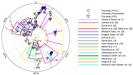
Figure 2.
Localizations of matchups from this study and several research areas of previous matchup studies evaluating chlorophyll-a satellite products. The blue circles, red dots and black triangles correspond to matchups from this study for chlorophyll-a measured by HPLC, fluorometry, and POC respectively.
2.3. Statistical Metrics
The MARD (mean absolute relative difference) and the MRD (mean relative difference) were used as statistic metrics for quantifying the uncertainty associated with satellite estimations:
where N is the number of points, while E and M represent the retrieved and measured values respectively. Since the arithmetic mean is sensitive to potential extreme values, the median relative difference (MedRD) and the median absolute relative difference (MedRAD) have been calculated as well. As the distribution of POC and chlorophyll-a follow a lognormal curve [39,40,41], statistics are also shown for the logarithmically transformed (base 10) data. The formulations of Seegers et al. [41] have been followed:
Please note that Equations (5)–(6) are dimensionless. Differences between chlorophyll-a retrieved from HPLC and from fluorometry were analysed using the MRD, the root mean square difference (RMSD) and the coefficient of determination (R) defined as per Ricker et al. [42]:
where E and M represent the chlorophyll-a measured from fluorometry and HPLC respectively.
3. Results
By applying all steps in the matchup procedure, a time window of ±12 h and using box 1 (mean of a 5 × 5 pixel box centered on the in situ location), a total of 73, 46 and 46 matchups were obtained for C, C and POC respectively. The concentrations of POC and chlorophyll-a (measured from HPLC) were in a typical range for the SO: between 36 and 257 mg m with a median of 89 mg m for POC and between 0.04 and 3.7 mg m with a median of 0.33 mg m for C [12,29,43]. Concentrations in chlorophyll-a measured from fluorometry (C) were slightly higher, ranging from 0.12 to 4.5 mg m with a median of 0.45 mg m. When comparing satellite retrieved values with in situ values, data points are scattered around the 1:1 line for C (with a median ratio of ∼0.9), whereas underestimations are observed for the C (median ratio of ∼0.5) and the POC (median ratio of ∼0.7) (Figure 3 and Figure 4). These observations are verified by the probability density distributions of log(C:C) from C, which are normally distributed around −0.05 compared to −0.31 for C and −0.13 for POC. Worth noting is that C:C and C:C ratios are similar to those obtained by Marrari et al. [30] in the Antarctic Peninsula region.
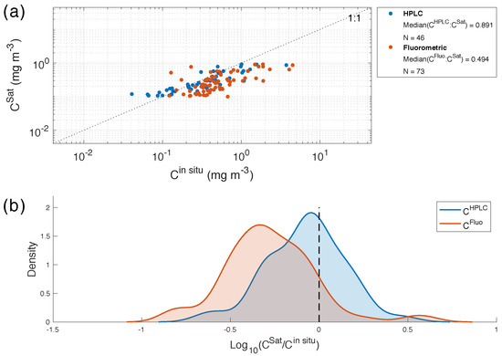
Figure 3.
(a) Comparison between measured (C) and retrieved (C) chlorophyll-a for box 1 with a time window of 12 h. Blue and orange dots indicate samples measured from HPLC (C) and fluorometry (C) respectively, while the dashed line shows the 1:1 relationship. (b) Probability density function of the logarithm base 10 of the ratio between C and C from fluorometry (blue line) and HPLC (orange line); with the statistics of the comparisons listed in Table 2.
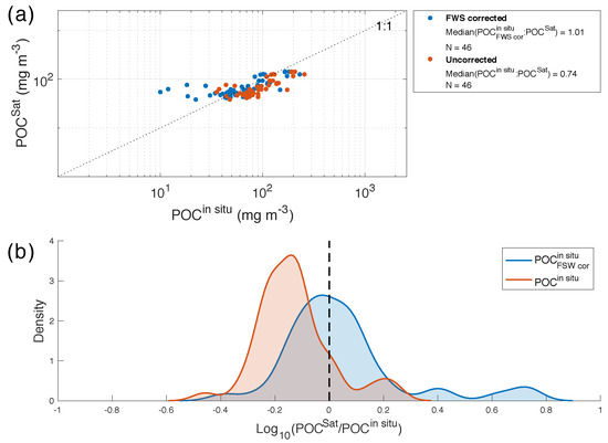
Figure 4.
(a) Comparison between measured POC (POC) and retrieved (POC) for box 1 with a time window of 12 h. Blue and orange dots indicate dry-blank corrected samples (POC) and filtered seawater corrected blanks (POC) respectively; the dashed line shows the 1:1 relationship. (b) Probability density function of the logarithm base 10 of the ratio between POC and POC (orange line) and POC (blue line); the statistics of the comparisons are listed in Table 2.
Similar results are obtained when statistics are performed for different averaging products in box 1 and 2 (see Section 2.2) and different time windows (±3 h, ±6 h, ±9 h and ±12 h) (Table 2). For example, using box 1 and a time window of ±12 h, the MRD and MARD between retrieved and in situ data were −6% and 36% for C, whereas higher differences were observed for C (MRD = −35%, MARD = 54%) and POC (MRD = −22%, MARD = 32%). Marrari et al. [30] similarly noted a larger bias using fluorometric measurements when comparing SeaWIFS daily chlorophyll-a data (resolution: ∼1 km/pixel from SeaDAS4.8, OC4v4 algorithm) with in situ chlorophyll-a from HPLC and fluorometric measurements in the Antarctic Peninsula, where the authors obtained a MRD of 12% for C and −45.2% for C. For the different time windows tested, the errors remained relatively constant for all different algorithms. Using a radius of 8 km centered on the in situ location (box 2) enabled an increase in the number of matchups without necessarily impacting the accuracy or bias. To elaborate, the number of matchups between box 1 and box 2 increased by an average factor of 1.4, while the medians of the ratio of the MARD and the MRD between box 2 and box 1 were 1 and 1.1 respectively. Surprisingly, in some instances there was a tendency for the accuracy of the algorithm to be slightly better using box 2. For instance, the MARD for C was 44% for box 1 and 35% for box 2 when using a time window of ±3 h. Note however that the difference between in situ concentrations of C between box 1 and box 2 were the highest as opposed to inter box comparisons of C and POC. To elaborate, the MARD between in situ concentrations for C in box 1 and box 2 was 8.4% while these diffrences were low for C (MARD = 3.2%) and POC (MARD = 3.6%). Thus, differences in the results observed between box 1 and 2 for C were likely due to variations in in situ concentrations. Indeed, algorithm performance has been known to differ according to variations in the range of concentration. To test this, an evaluation of the errors according to different concentration ranges was performed utilising a time window of ±12 h and box 1 (Table 3). For chlorophyll-a, the limits were chosen to separate the Color Index (<0.2 mg m; [44]) and OC3M algorithms (see Appendix A). For POC, the concentration limits correspond to the first and third quartile (Q1 = 67 mg m and Q3 = 124 mg m). Results confirm that errors in the chlorophyll-a product are more sensitive to the range of concentration than the POC product. The coefficient of variation of the MARD was 12% for C and 32% for C, whereas it was of 3% for POC. However, we note that no significant variation in the statistics was observed when using only the OC3M algorithm instead of the blended version. For instance, the MARD increased by ∼1% using exclusively the OCx model (C < 0.2; N = 13).
Table 3.
Statistics of the comparison between satellite and in situ values for different ranges in concentration. A time window of 12 h and box 1 was used for the extraction procedure.
4. Discussion
4.1. Satellite Versus In Situ Chlorophyll-a Comparison
There is a recognised need in the user community for ocean colour products to be regionally optimised and their uncertainties well characterised [45]. Despite previous conclusions of a poor performance of the ocean colour chlorophyll-a product (with a typical underestimate of 50%) from the majority of validation studies performed in the SO, results from this study show good agreement between chlorophyll-a retrievals from MODIS and in situ HPLC derived chlorophyll-a. These results are in agreement with only two other studies in the literature [29,30]. The more recent study from Haëntjens et al. [29] focused on in situ data derived from floats, which themselves have significant uncertainties in estimating chlorophyll-a, primarily due to variability in the chlorophyll-a to fluorescence yield that changes during the floats life time in response to adjustments in photophysiology, nutrients, temperature and species composition [46,47,48]. They however tested the float bias using an independent data set of 97 matchups of HPLC derived chlorophyll-a (from NASA’s SeaBASS database) with MODIS OCI, which showed similar results to ours, supporting their conclusion that the default algorithm to estimate chlorophyll-a from NASA performs well in the SO, and that a regional specific algorithm is not required. Our results from an extensive in situ database of HPLC derived chlorophyll (using consistent methods and analysis) covering a broad regional and seasonal range and stricter matchup criteria, supports this conclusion. In addition, our dataset of co-located fluorescence and HPLC derived chlorophyll allows us to go one step further and interrogate possible reasons for the average factor of 0.5 underestimate typical of previous validation studies.
4.2. Comparison of HPLC and the Fluorometric Chlorophyll-a Methods
HPLC and fluorometry are two distinct methods currently used to measure the concentration of chlorophyll-a in marine environments. The HPLC method separates phytoplankton pigments in order of polarity upon passage through a column [33], with the most polar pigments removed earlier than the less polar pigments [34,49]. The fluorometric method uses the capacity of chlorophyll-a pigments to fluoresce in the red part of the spectrum when they are excited by blue light. Briefly, fluorescence of in vivo chlorophyll-a is measured by irradiating a water sample in the blue-green region of the spectrum (∼440 nm), following which, the amount of energy fluoresced in the red region (∼685 nm) as a result of light interactions with the chlorophyll molecules, is measured by a detector to produce raw fluorescence units (RFU). The RFU are then converted into chlorophyll-a concentration by means of a calibration curve pre-established with a range of chlorophyll-a standards, where the curve represents an ideal case of fluorescence measurements being linearly related to chlorophyll-a concentrations. Two conditions have to be encountered to satisfy this case: (i) the excitation energy (mol photon m s nm) is saturating and constant among measurements and (ii) the spectral chlorophyll-a specific absorption coefficient (m mg Chl) and fluorescence quantum yield product (mol photons fluoresced mol photons absorbed) have to be linearly related to fluorescence. It is however well known that the second postulate is not always satisfied [46,48,50]. Firstly, because the chlorophyll-a specific absorption coefficient depends on cell size, pigment concentration, the package effect and pigment composition [51,52]; and secondly, because fluorescence quantum yield changes as a function of species, nutritional status, ambient light and light history [46,48,53]. In addition, the integrity of fluorescence measurements may suffer from interference from the presence of significant amounts of chlorophyll-b, chlorophyll-c and degradation products (i.e., phaeopigments phaeophytin-a and phaeophorbide-a), which fluoresce in a similar spectral region as chlorophyll-a; this overlap may result in overestimates of the chlorophyll-a concentration (as in our case when using the non-acidification technique) and/or an underestimation (if the acidification technique is used) [30,31,32,48,49,54,55,56,57]. To elaborate, The acidification technique follows the method of Holm-Hansen et al. [58], where the impacts on fluorescence by phaeopigments are quantified by acidifying the sample, which converts all of the chlorophyll-a to phaeopigments. The difference between the two fluorescnece measurements (before and after acidification) thus reflects the total amount of chlorophyll-a in the sample. However, the acidification process results in an underestimate of chlorophyll-a in the presence of chlorophyll-b as the acidification step converts all chllorophyll-b to pheophytin b which has an overlapping emission spectra with pheophytin a [32]. To improve the accuracy of fluorescence measurements the Welschmeyer, [32] non-acidification method (used here) was optimised to avoid the overlapping phenomena by implementing a narrow band width optical approach to measured fluorescence that provides maximum sensitivity to chlorophyll-a while maintaining desensitized responses to chlorophyll-c, chlorophyll-b and phaeopigments. However, biases are still present making the HPLC method the more reliable method for quantifying chlorophyll-a concentration [32,48,55].
4.3. C vs. C
Coincident HPLC and fluorometric measurements were collected from different locations and time periods in the SO (Table 1). Results show a typical overestimation of C when compared to C, with median C:C ratios that range from 1.1 (SANAE 48) to 2.8 (ACE) (all data median = 1.5) (Table 4; Figure 5). Linear regression slopes between C and C ranged from 0.85 to 2.21 while the MRD ranged from 8% to 284%. Such discrepancies between methods have been reported previously in the literature [7,30,31,32,48,49,54,55,56,57], which could be explained by concentrations of chlorophyll-b or chlorophyll-c that vary regionally with different dominant species composition [30,54,55,56,57,59,60]. Worth noting is that ACE is the only research cruise that collected samples from the continental margin region around Antarctica (excluding ACE data puts the “all cruise” median C/ C at 1.37 instead of 1.5). In an attempt to determine the drivers of this discrepancy, the data have been analysed according to latitude. Results indicate that the MRD between C and C is linked to progression in latitude, total biomass (estimated from C) and the proportion of chlorophyll-c and fucoxanthin (Table 5). Such pigments are found in the taxa Bacillariophytes (diatoms) and Haptophytes (e.g., Phaeocystis antarctica), which typically dominate the SO [61,62,63]. The role of chlorophyll-c and fucoxanthin pigments are crucial in marine phytoplankton environments as their absorption covers the blue-green part of the light spectrum [64], which is prevalent in marine environments. However, while chlorophyll-c and fucoxanthin are found in both taxa, fucoxanthin is considered a marker pigment for the diatoms, with much lower concentrations being typical of the SO strain of Phaeocystis [62,65]. Results therefore suggest that diatoms are the dominant source of chlorophyll-c and that their presence is primarily responsible for the observed range in C:C ratios presented in Table 5. The dominance of specific species in certain regions is mainly driven by sea surface temperature, sea ice presence, grazing pressure and water column structure which influences both nutrient and light availability ([63,66] and references therein). For diatom species, favorable growth conditions are associated with high nutrient concentrations (nitrate, silicate and iron) [63,67,68]. In the SO, the Polar Front with a mean position in the Atlantic SO of 54S [69] forms an important transitional boundary, south of which high silicate concentrations prevail and diatoms typically dominate [68,70]. In addition, diatoms typically dominate in regions with shallow mixed layers that are characteristic of stratified waters (e.g., from ice melt) that provide a high light environment by allowing dense cells to remain suspended in the illuminated surface waters ([71] and references therein). It is thus recommended that in regions where diatoms dominate and a high proportion of chlorophyll-c is anticipated (e.g., the SO), that HPLC be the method implemented for chlorophyll-a analysis.
Table 4.
Statistics of the relation between chlorophyll-a measured from HPLC and fluorometry for each expedition. The number of observations (N), the slope (a), the intercept (b) and their standard deviations (a and b) and coefficients of determination (R) of the linear regression are indicated. RMSD is the root mean square difference and MRD is the mean relative difference (see Section 2.3 for formulations).
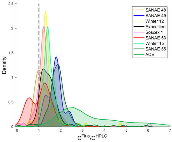
Figure 5.
Probability density function of the ratio between chlorophyll-a measured from fluorometry (C) and HPLC (C). Each color corresponds to a specific expedition.
Table 5.
Statistics of the relationship between chlorophyll-a measured from HPLC and fluorometry for different ranges of latitude, the proportion of chlorophyll-c and Fucoxanthin is also indicated. The number of observations (N), the slope (a), the intercept (b) and their standard deviations (a and b) and the coefficient of determination (R) of the linear regression are indicated. RMSD is the root mean square difference and MRD is the mean relative difference (see Section 2.3 for formulations).
4.4. Satellite Versus In Situ POC Comparison
An intercomparison and validation study of various ocean colour POC algorithms by Evers-King et al. [45] found that the Stramski et al. [72] algorithm (applied here), performed well and consistently across a broad range in POC concentration (2.7–8 097 mg m) and across different water types, with the majority of pixels falling within an error range of 30%. The SO specific matchup performed here, across a lower range in POC (36–257 mg m) found a 30% underestimate in the Stramski et al. [72] algorithm, which was verified by the probability density distribution offset in POC:POC ratios of −0.13 (Figure 4). However, a number of studies have highlighted the issue of different methodologies for treating POC blanks as a possible source of bias, particularly at low POC concentrations. Cetinic et al. [73] (and references therein) show that the effect of dissolved organic carbon (DOC) adsorption onto filters (if not accounted for with an adequate blank correction) can result in an overestimate in POC of between 11 and 25 mg m. On the most recent SO cruise (ACE, Table 1), DOC adsorption onto filters was tested by passing filtered seawater through an unused, pre combusted GF/F filter to obtain a filtered seawater blank of 25.7 mg m. On ACE, the difference between the FSW-blank and the mean dry-filter-blank (i.e., the DOC contribution) was 18.92 mg m. If this is assumed to be representative of DOC adsorption and subtracted from all SO cruises in Table 1 (in addition to the dry-filter-blank), the revised matchup with satellite POC results in a median POC:POC ratio of 1.01 (Figure 4). These results suggest a robust performance of the Stramski et al. [72] POC algorithm in the SO and highlight the requirement for revised JGOFS POC protocols to include a blank exposed to filtered seawater [74].
5. Conclusions
The standard MODIS L2 chlorophyll-a and POC products were evaluated by comparing satellite retrievals with an in situ dataset encompassing a broad geographical and seasonal range. The database included POC concentrations (mg m) and chlorophyll-a concentrations (mg m) measured from both fluorometric and HPLC methods. Using strict matchup criteria of a time window of ±12 h and the mean of a 5 × 5 pixel box centered on the in situ location. The median of the C:C ratios were 0.89 for C (N = 46) and 0.49 for C (N = 73). The mean relative difference and mean relative absolute difference were −5.8% and 36.2% for C whereas they were −35% and 54% for C. Note that an increase in the spatio-temporal resolutions to a time window of ±12 h and to a radius of 8 km around the in situ sample localization did not impact the results.
The consensus observed in our study between C and C suggests that the MODIS global chlorophyll-a algorithm performs well in the SO, which agrees with a recent publication by Haëntjens et al. [29]. The comparatively poor performance of C supports the more common factor of ∼0.5 difference between retrieved and measured values of chlorophyll-a obtained by most previous validation studies in the SO, that were typically done with chlorophyll-a measured from fluorometry rather than HPLC. Similarly to Marrari et al. [30], our results suggest that the typical overestimation of C was due to the presence of chlorophyll-c pigments from diatom species. The median relative difference of −26% observed for the POC to POC comparison has to be interpreted carefully as this underestimate is likely due to a methodological bias from an inadequate blank correction applied to in situ POC samples. If an assumption is made on the representativeness of the contribution of DOC adsorption onto POC filters (18.92 mg m), then the performance of the satellite algorithm improves to a median of 1.01 (median relative difference and median relative absolute difference of 1% and 23% respectively).
These results highlight the importance of accurately calibrating fluorescence measurements and promotes the use of the HPLC method of chlorophyll-a analysis, particularly in regions where diatoms are known to dominate and despite the high costs involved. In addition, as noted by Boss et al. [53], the best calibration should be more often and as close as possible in time and space to the sampled area. Similarly, results highlight the need for community consensus for a standard protocol for POC analysis that includes an FSW-blank.
Author Contributions
Conceptualization, W.M., S.J.T. and S.B.; Data Curation, W.M., S.J.T. and T.J.R.-K.; Formal Analysis, W.M.; Funding Acquisition, S.J.T.; Investigation, W.M., S.J.T. and S.B.; Methodology, W.M., S.J.T., S.B., G.W. and M.E.S.; Project Administration, S.J.T.; Resources, S.J.T.; Software, W.M. and G.W.; Supervision, S.J.T. and S.B.; Validation, W.M. and T.J.R.-K.; Visualization, W.M.; Writing—Original Draft, W.M.and S.J.T.; Writing—Review & Editing, W.M., S.J.T., S.B., G.W., T.J.R.-K. and M.E.S.
Funding
This work was undertaken as part of the CSIR’s Southern Ocean Carbon and Climate Observatory (SOCCO) (http://socco.org.za). This work was supported by CSIR’s Parliamentary Grant (SNA2011112600001), the NRF South African National Antarctic Programme (SANAP) grants (SNA2007051100001, SNA2011120800004, SNA14071475720), the European Commission 7th Framework program through the GreenSeas Collaborative Project, FP7-ENV-2010 contract No. 265294 and the ACE scientific expedition carried out under the auspices of the Swiss Polar Institute, supported by funding from the ACE Foundation and Ferring Pharmaceuticals.
Acknowledgments
We would like to thank our funders and the captains and crews of the S.A. Agulhas, S.A. Agulhas II and RV Akademic Tryoshnikov for their professional support throughout the cruises. This work was undertaken as part of the CSIR’s Southern Ocean Carbon and Climate Observatory (SOCCO) (http://socco.org.za). We thank the anonymous reviewers for their valuable comments and suggestions.
Conflicts of Interest
The authors declare no conflict of interest.
Abbreviations
The following abbreviations are used in this manuscript:
| APFZ | Antarctic Polar Front Zone |
| C | Chlorophyll-c concentration |
| C | Chlorophyll-a concentration measured by Fluorometry |
| C | Chlorophyll-a concentration measured by High Performance Liquid Chromatography |
| C | Chlorophyll-a concentration retrieved by satellite |
| CDOM | Colored Dissolved Organic Matter |
| CTD | Conductivity-Temperature-Depth |
| CV | Coefficient of Variation |
| DOC | Dissolved Organic Carbon |
| EOS | Earth Observing System |
| FSW | filtered seawater |
| HPLC | High Performance Liquid Chromatography |
| IOP | Inherent Optical Properties |
| JGOFS | Joint Global Ocean Flux Studies |
| MLD | Mixed Layer Depth |
| MODIS | MODerate resolution Imaging Spectroradiometer |
| MRAD | Mean Relative Absolute Difference |
| MRD | Mean Relative Difference |
| NASA | National Aeronautics and Space Administration |
| POC | Particulate Organic Carbon |
| POC | in situ concentration in Particulate Organic Carbon |
| POC | Particulate Organic Carbon concentration retrieved by satellite |
| RFU | Raw Fluorescence Units |
| RMSD | Root Mean Square Difference |
| SeaWIFS | Sea-viewing Wide Field-of-view Sensor |
| SO | Southern Ocean |
| SOCCOM | Southern Ocean Carbon and Climate Observations and Modeling |
| VIIRS | Visible Infrared Imager Radiometer Suite |
Appendix A
Appendix Algorithms Description
The current chlorophyll-a algorithm is a blend between the standard OCx band ratio algorithm (named OC3M for Aqua MODIS) and the Color Index (CI) of Hu et al. [44]:
with:
where R() is the remote sensing reflectance (R) at 547 nm, and R() is the greatest R between 443 and 488 nm. The CI algorithm is defined as follows:
with:
where , and represent the closest wavelength to 443, 555 and 670 nm respectively. A weighted model (WM) is used to blend between the CI and OC3M algorithms at chlorophyll-a concentrations between 0.15 and 0.20 mg m, while only the CI and OC3M are used at concentrations of <0.15 and >0.20 mg m respectively. The weighted model is defined as follows:
The current POC algorithm was developed by Stramski et al. [72] and is defined as follows:
References
- Raven, J.A.; Falkowski, P.G. Oceanic sinks for atmospheric CO2. Plant Cell Environ. 1999, 22, 741–755. [Google Scholar] [CrossRef]
- Sabine, C.L.; Feely, R.A.; Gruber, N.; Key, R.M.; Lee, K.; Bullister, J.L.; Wanninkhof, R.; Wong, C.S.L.; Wallace, D.W.R.; Tilbrook, B.; et al. The oceanic sink for anthropogenic CO2. Science 2004, 305, 367–371. [Google Scholar] [CrossRef] [PubMed]
- Khatiwala, S.; Primeau, F.; Hall, T. Reconstruction of the history of anthropogenic CO2 concentrations in the ocean. Nature 2009, 346–349, 554–577. [Google Scholar] [CrossRef] [PubMed]
- Takahashi, T.; Sutherland, S.C.; Wanninkhof, R.; Sweeney, C.; Feely, R.A.; Chipman, D.W.; Hales, B.; Friederich, G.; Chavez, F.; Sabine, C. Climatological mean and decadal change in surface ocean pCO2, and net sea–air CO2 flux over the global oceans. Deep Sea Res. Part 2 Top. Stud. Oceanogr. 2009, 56, 554–577. [Google Scholar] [CrossRef]
- Frölicher, T.L.; Sarmiento, J.L.; Paynter, D.J.; Dunne, J.P.; Krasting, J.P.; Winton, M. Dominance of the Southern Ocean in Anthropogenic Carbon and Heat Uptake in CMIP5 Models. J. Clim. 2015, 28, 862–886. [Google Scholar] [CrossRef]
- Sigman, D.M.; Boyle, E.A. Glacial/interglacial variations in atmospheric carbon dioxide. Nature 2000, 859–869, 554–577. [Google Scholar] [CrossRef]
- Pereira, E.S.; Garcia, C.A. Evaluation of satellite-derived MODIS chlorophyll algorithms in the northern Antarctic Peninsula. Deep Sea Res. Part 2 Top. Stud. Oceanogr. 2018, 149, 124–137. [Google Scholar] [CrossRef]
- Muller-Karger, F.; Varela, R.; Thunell, R.; Astor, Y.; Zhang, H.; Luerssen, R.; Hu, C. Processes of coastal upwelling and carbon flux in the Cariaco Basin. Deep Sea Res. Part 2 Top. Stud. Oceanogr. 2004, 51, 927–943. [Google Scholar] [CrossRef]
- Hu, C.; Muller-Karger, F.E.; Taylor, C.J.; Carder, K.L.; Kelble, C.; Johns, E.; Heil, C.A. Red tide detection and tracing using MODIS fluorescence data: A regional example in SW Florida coastal waters. Remote Sens. Environ. 2005, 97, 311–321. [Google Scholar] [CrossRef]
- Mitchell, B.G.; Holm-Hansen, O. Bio-optical properties of Antarctic Peninsula waters: Differentiation from temperate ocean models. Deep Sea Res. A 1991, 38, 1009–1028. [Google Scholar] [CrossRef]
- Sullivan, C.W.; Arrigo, K.R.; McClain, C.R.; Comiso, J.C.; Firestone, J. Distributions of phytoplankton blooms in the Southern Ocean. Science 1993, 262, 1832–1837. [Google Scholar] [CrossRef] [PubMed]
- Arrigo, K.R.; Worthen, D.; Schnell, A.; Lizotte, M.P. Primary production in Southern Ocean waters. J. Geophys. Res. 2008, 103, 15587–15600. [Google Scholar] [CrossRef]
- Moore, J.K.; Abbott, M.R.; Richman, J.G.; Smith, W.O.; Cowles, T.J.; Coale, K.H.; Gardner, W.D.; Barber, R.T. SeaWiFS satellite ocean color data from the Southern Ocean. Geophys. Res. Lett. 1999, 26, 1465–1468. [Google Scholar] [CrossRef]
- Dierssen, H.M.; Smith, R.C. Bio-optical properties and remote sensing ocean color algorithms for Antarctic Peninsula waters. J. Geophys. Res. Oceans 2000, 105, 26301–26312. [Google Scholar] [CrossRef]
- Reynolds, R.A.; Stramski, D.; Mitchell, B.G. A chlorophyll-dependent semianalytical reflectance model derived from field measurements of absorption and backscattering coefficients within the Southern Ocean. J. Geophys. Res. Oceans 2001, 106, 7125–7138. [Google Scholar] [CrossRef]
- Clementson, L.A.; Parslow, J.S.; Turnbull, A.R.; McKenzie, D.C.; Rathbone, C.E. Optical properties of waters in the Australasian sector of the Southern Ocean. J. Geophys. Res. Oceans 2001, 106, 31611–31625. [Google Scholar] [CrossRef]
- Barbini, R.; Colao, F.; Fantoni, R.; Fiorani, L.; Palucci, A.; Artamonov, E.S.; Galli, M. Remotely sensed primary production in the western Ross Sea: Results of in situ tuned models. Remote Sens. Environ. 2003, 15, 77–84. [Google Scholar] [CrossRef]
- Holm-Hansen, O.; Kahru, M.; Hewes, C.D.; Kawaguchi, S.; Kameda, T.; Sushin, V.A.; Krasovski, I.; Priddle, J.; Korb, R.; Hewitt, R.P.; et al. Temporal and spatial distribution of chlorophyll-a in surface waters of the Scotia Sea as determined by both shipboard measurements and satellite data. Deep Sea Res. Part 2 Top. Stud. Oceanogr. 2004, 51, 1323–1331. [Google Scholar] [CrossRef]
- Garcia, C.A.E.; Garcia, V.M.T.; McClain, C.R. Evaluation of SeaWiFS chlorophyll algorithms in the Southwestern Atlantic and Southern Oceans. Remote Sens. Environ. 2005, 95, 125–137. [Google Scholar] [CrossRef]
- Gregg, W.W.; Casey, N.W. Global and regional evaluation of the SeaWiFS chlorophyll data set. Remote Sens. Environ. 2004, 93, 463–479. [Google Scholar] [CrossRef]
- Korb, R.E.; Whitehouse, M.J.; Ward, P. SeaWiFS in the southern ocean: Spatial and temporal variability in phytoplankton biomass around South Georgia. Deep Sea Res. Part 2 Top. Stud. Oceanogr. 2004, 51, 99–116. [Google Scholar] [CrossRef]
- Mitchell, B.G.; Kahru, M. Bio-optical algorithms for ADEOS-2 GLI. J. Remote Sens. Soc. Jpn. 2009, 29, 80–85. [Google Scholar] [CrossRef]
- Kahru, M.; Mitchell, B.G. Blending of ocean colour algorithms applied to the Southern Ocean. Remote Sens. Lett. 2010, 1, 119–124. [Google Scholar] [CrossRef]
- Szeto, M.; Werdell, P.J.; Moore, T.S.; Campbell, J.W. Are the world’s oceans optically different? J. Geophys. Res. Oceans 2011, 116, 1–14. [Google Scholar] [CrossRef]
- Guinet, C.; Xing, X.; Walker, E.; Monestiez, P.; Marchand, S.; Picard, B.; Jaud, T.; Authier, M.; Cotté, C.; Dragon, A.; et al. Calibration procedures and first data set of Southern Ocean chlorophyll a profiles collected by elephant seals equipped with a newly developed CTD-fluorescence tags. Earth Syst. Sci. Data 2013, 5, 15–29. [Google Scholar] [CrossRef]
- Johnson, R.; Strutton, P.G.; Wright, S.W.; McMinn, A.; Meiners, K.M. Three improved satellite chlorophyll algorithms for the Southern Ocean. J. Geophys. Res. Oceans 2013, 118, 3694–3703. [Google Scholar] [CrossRef]
- Dierssen, H.M. Perspectives on empirical approaches for ocean color remote sensing of chlorophyll in a changing climate. Proc. Natl. Acad. Sci. USA 2010, 107, 17073–17078. [Google Scholar] [CrossRef]
- Bailey, S.W.; Werdell, P.J. A multi-sensor approach for the on-orbit validation of ocean color satellite data products. Remote Sens. Environ. 2006, 102, 12–23. [Google Scholar] [CrossRef]
- Haëntjens, N.; Boss, E.; Talley, L.D. Revisiting Ocean Color algorithms for chlorophyll a and particulate organic carbon in the Southern Ocean using biogeochemical floats. J. Geophys. Res. Oceans 2017, 122, 6583–6593. [Google Scholar] [CrossRef]
- Marrari, M.; Hu, C.; Daly, K. Validation of SeaWiFS chlorophyll a concentrations in the Southern Ocean: A revisit. Remote Sens. Environ. 2006, 105, 367–375. [Google Scholar] [CrossRef]
- Gibbs, C.F. Chlorophyll b interference in the fluorometric determination of chlorophyll a and ’phaeo-pigments’. Mar. Freshw. Res. 1979, 30, 597–606. [Google Scholar] [CrossRef]
- Welschmeyer, N.A. Fluorometric analysis of chlorophyll a in the presence of chlorophyll b and pheopigments. Limnol. Oceanog. 1994, 39, 1985–1992. [Google Scholar] [CrossRef]
- Ras, J.; Claustre, H.; Uitz, J. Spatial variability of phytoplankton pigment distributions in the Subtropical South Pacific Ocean: Comparison between in situ and predicted data. Biogeosciences 2008, 5, 353–369. [Google Scholar] [CrossRef]
- Knap, A.H.; Michaels, A.; Close, A.R.; Ducklow, H.; Dickson, A.G. Protocols for the Joint Global Ocean Flux Study (JGOFS) Core Measurements; Reprint of Intergovernmental Oceanographic Commission Manuals and Guides, No. 29; UNESCO: Paris, France, 1994; p. 170. [Google Scholar]
- Ocean Color Feature. Available online: http://oceancolor.gsfc.nasa.gov (accessed on 4 July 2019).
- NASA Goddard Space Flight Center, Ocean Ecology Laboratory, Ocean Biology Processing Group. Moderate-resolution Imaging Spectroradiometer (MODIS) Aqua Ocean Color Data; 2018 Reprocessing; NASA OB.DAAC: Greenbelt, MD, USA, 2018. [CrossRef]
- Level 2 Ocean Color Flags. Available online: https://oceancolor.gsfc.nasa.gov/atbd/ocl2flags/ (accessed on 4 July 2019).
- Zheng, G.; DiGiacomo, P.M. Uncertainties and applications of satellite-derived coastal water quality products. Prog. Oceanogr. 2017, 159, 45–72. [Google Scholar] [CrossRef]
- Campbell, J.W. The lognormal distribution as a model for bio-optical variability in the sea. J. Geophys. Res. Oceans 1995, 100, 13237–13254. [Google Scholar] [CrossRef]
- Campbell, J.W.; O’Reilly, J.E. Metrics for Quantifying the Uncertainty in a Chlorophyll Algorithm: Explicit equations and examples using the OC4. v4 algorithm and NOMAD data. In Proceedings of the Ocean Color Bio-Optical Algorithm Mini (OCBAM) Workshop, New England Center, Southborough, MA, USA, 27–29 September 2005; pp. 1–15. [Google Scholar]
- Seegers, B.N.; Stumpf, R.P.; Schaeffer, B.A.; Loftin, K.A.; Werdell, P.J. Performance metrics for the assessment of satellite data products: An ocean color case study. Opt. Express 2018, 26, 7404–7422. [Google Scholar] [CrossRef] [PubMed]
- Ricker, W.E. Linear regressions in fishery research. J. Fish. Res. Board Can. 1973, 30, 409–434. [Google Scholar] [CrossRef]
- Stramski, D.; Reynolds, R.A.; Kahru, M.; Mitchell, B.G. Estimation of particulate organic carbon in the ocean from satellite remote sensing. Sciences 1999, 285, 239–242. [Google Scholar] [CrossRef]
- Hu, C.; Lee, Z.; Franz, B. Chlorophyll a algorithms for oligotrophic oceans: A novel approach based on three-band reflectance difference. J. Geophys. Res. Oceans 2012, 117. [Google Scholar] [CrossRef]
- Evers-King, H.; Martinez-Vicente, V.; Brewin, R.J.W.; Dall’Olmo, G.; Hickman, A.E.; Jackson, T.; Kostadinov, T.S.; Krasemann, H.; Loisel, H.; Röttgers, R.; et al. Validation and intercomparison of ocean color algorithms for estimating particulate organic carbon in the oceans. Front. Mar. Sci. 2017, 4, 1–19. [Google Scholar] [CrossRef]
- Cullen, J.J. The deep chlorophyll maximum: Comparing vertical profiles of chlorophyll a. Can. J. Fish. Aquat. Sci. 1982, 39, 791–803. [Google Scholar] [CrossRef]
- Proctor, C.W.; Roesler, C.S. New insights on obtaining phytoplankton concentration and composition from in situ multispectral Chlorophyll fluorescence. Limnol. Oceanogr. Methods 2010, 8, 695–708. [Google Scholar] [CrossRef]
- Roesler, C.; Uitz, J.; Claustre, H.; Boss, E.; Xing, X.; Organelli, E.; Briggs, N.; Bricaud, A.; Schmechtig, C.; Poteau, A.; et al. Recommendations for obtaining unbiased chlorophyll estimates from in situ chlorophyll fluorometers: A global analysis of WET Labs ECO sensors. Limnol. Oceanogr. Methods 2017, 15, 572–585. [Google Scholar] [CrossRef]
- Kumari, B. Comparison of high performance liquid chromatography and fluorometric ocean colour pigments. J. Indian Soc. Remote 2005, 33, 541–546. [Google Scholar] [CrossRef]
- Kahru, M.; Mitchell, B.G. Chlorophyll a fluorescence in marine centric diatoms: Responses of chloroplasts to light and nutrient stress. Mar. Biol. 1973, 23, 39–46. [Google Scholar] [CrossRef]
- Morel, A.; Bricaud, A. Theoretical results concerning light absorption in a discrete medium, and application to specific absorption of phytoplankton. Deep Sea Res. A 1981, 28, 1375–1393. [Google Scholar] [CrossRef]
- Bricaud, A.; Morel, A.; Prieur, L. Optical efficiency factors of some phytoplankters. Limnol. Oceanogr. 1983, 28, 816–832. [Google Scholar] [CrossRef]
- Boss, E.; Swift, D.; Taylor, L.; Brickley, P.; Zaneveld, R.; Riser, S.; Perry, M.J.; Strutton, P.G. Observations of pigment and particle distributions in the western North Atlantic from an autonomous float and ocean color satellite. Limnol. Oceanogr. 2008, 53, 2112–2122. [Google Scholar] [CrossRef]
- Lorenzen, C.J. Chlorophyll b in the eastern North Pacific Ocean. Deep Sea Res. A 1981, 28, 1049–1056. [Google Scholar] [CrossRef]
- Trees, C.C.; Kennicutt, M.C., II; Brooks, J.M. Errors associated with the standard fluorimetric determination of chlorophylls and phaeopigments. Mar. Chem. 1985, 17, 1–12. [Google Scholar] [CrossRef]
- Bianchi, T.S.; Lambert, C.; Biggs, D.C. Distribution of chlorophyll a and phaeopigments in the northwestern Gulf of Mexico: A comparison between fluorometric and high-performance liquid chromatography measurements. Bull. Mar. Sci. 1995, 56, 25–32. [Google Scholar]
- Dos Santos, A.C.A.; Calijuri, M.D.C.; Moraes, E.M.; Adorno, M.A.T.; Falco, P.B.; Carvalho, D.P.; Deberdt, G.L.B.; Benassi, S.F. Comparison of three methods for Chlorophyll determination: Spectrophotometry and Fluorimetry in samples containing pigment mixtures and spectrophotometry in samples with separate pigments through High Performance Liquid Chromatography. Acta Limnol. Bras. 2003, 15, 7–18. [Google Scholar]
- Holm-Hansen, O.; Lorenzen, C.J.; Holmes, R.W.; Strickland, J.D. Fluorometric determination of chlorophyll. ICES J. Mar. Sci. 1965, 30, 3–15. [Google Scholar] [CrossRef]
- Jeffrey, S.W. A report of green algal pigments in the central North Pacific Ocean. Mar. Biol. 1976, 37, 33–37. [Google Scholar] [CrossRef]
- Bidigare, R.R.; Frank, T.J.; Zastrow, C.; Brooks, J.M. The distribution of algal chlorophylls and their degradation products in the Southern Ocean. Deep Sea Res. A 1986, 33, 923–937. [Google Scholar] [CrossRef]
- Parsons, T.R.; Takahashi, M.; Hargrave, B. Biological Oceanographic Processes, 3rd ed.; Oxford Pergamon Press: Oxford, UK, 1984; pp. 40–50. ISBN 0-08-030766-3. [Google Scholar]
- Arrigo, K.R.; Mills, M.M.; Kropuenske, L.R.; van Dijken, G.L.; Alderkamp, A.C.; Robinson, D.H. Photophysiology in two major Southern Ocean phytoplankton taxa: Photosynthesis and growth of Phaeocystis antarctica and Fragilariopsis cylindrus under different irradiance levels. Integr. Comp. Biol. 2010, 50, 950–966. [Google Scholar] [CrossRef] [PubMed]
- Mendes, C.R.B.; de Souza, M.S.; Garcia, V.M.T.; Leal, M.C.; Brotas, V.; Garcia, C.A.E. Dynamics of phytoplankton communities during late summer around the tip of the Antarctic Peninsula. Deep Sea Res. Part 1 Oceanogr. Res. Pap. 2012, 65, 1–14. [Google Scholar] [CrossRef]
- Papagiannakis, E.; van Stokkum, I.H.M.; Fey, H.; Buchel, C.; van Grondelle, R. Spectroscopic characterization of the excitation energy transfer in the fucoxanthin–chlorophyll protein of diatoms. Photosynth. Res. 2005, 86, 241–250. [Google Scholar] [CrossRef] [PubMed]
- Vaulot, D.; Birrien, J.L.; Marie, D.; Casotti, R.; Veldhuis, M.J.W.; Kraay, G.W.; Chrétiennot-Dinet, M.J. Morphology, ploidy, pigment composition, and genome size of cultured strains of Phaeocystis (Prymnesiophycea). J. Phycol. 1994, 30, 1022–1035. [Google Scholar] [CrossRef]
- Crosta, X.; Romero, O.; Armand, L.K.; Pichon, J.J. The biogeography of major diatom taxa in Southern Ocean sediments: 2. Open ocean related species. Palaeogeogr. Palaeoclimatol. Palaeoecol. 2005, 223, 66–92. [Google Scholar] [CrossRef]
- Boyd, P.W. Environmental factors controlling phytoplankton processes in the Southern Ocean. J. Phycol. 2002, 38, 844–861. [Google Scholar] [CrossRef]
- Coale, K.H.; Johnson, K.S.; Chavez, F.P.; Buesseler, K.O.; Barber, R.T.; Brzezinski, M.A.; Cochlan, W.P.M.; Millero, F.J.; Falkowski, P.G.; Bauer, J.E.; et al. Southern Ocean iron enrichment experiment: Carbon cycling in high-and low-Si waters. Science 2004, 304, 408–414. [Google Scholar] [CrossRef] [PubMed]
- Swart, S.; Speich, S. An altimetry-based gravest empirical mode south of Africa: 2. Dynamic nature of the Antarctic Circumpolar Current fronts. J. Geophys. Res. Oceans 2010, 115. [Google Scholar] [CrossRef]
- Trull, T.W.; Bray, S.G.; Manganini, S.J.; Honjo, S.; François, R. Moored sediment trap measurements of carbon export in the Subantarctic and Polar Frontal zones of the Southern Ocean, south of Australia. J. Geophys. Res. Oceans 2001, 106, 31489–31509. [Google Scholar] [CrossRef]
- Lindenschmidt, K.E.; Chorus, I. The effect of water column mixing on phytoplankton succession, diversity and similarity. J. Plankton Res. 1998, 20, 1927–1951. [Google Scholar] [CrossRef]
- Stramski, D.; Reynolds, R.A.; Babin, M.; Kaczmarek, S.; Lewis, M.R.; Röttgers, R.; Sciandra, A.; Stramska, M.; Twardowski, M.S.; Franz, B.A.; et al. Relationships between the surface concentration of particulate organic carbon and optical properties in the eastern South Pacific and eastern Atlantic Oceans. Biogeosciences 2008, 5, 171–201. [Google Scholar] [CrossRef]
- Cetinić, I.; Perry, M.J.; Briggs, N.T.; Kallin, E.; D’Asaro, E.A.; Lee, C.M. Particulate organic carbon and inherent optical properties during 2008 North Atlantic Bloom Experiment. J. Geophys. Res. Oceans 2012, 117, 13237–13254. [Google Scholar] [CrossRef]
- Gardner, W.D.; Richardson, M.J.; Carlson, C.A.; Hansell, D.; Mishonov, A.V. Determining true particulate organic carbon: Bottles, pumps and methodologies. Deep Sea Res. Part 2 Top. Stud. Oceanogr. 2003, 50, 655–674. [Google Scholar] [CrossRef]
© 2019 by the authors. Licensee MDPI, Basel, Switzerland. This article is an open access article distributed under the terms and conditions of the Creative Commons Attribution (CC BY) license (http://creativecommons.org/licenses/by/4.0/).