Abstract
Sea ice leads (fractures) play a critical role in the exchange of mass and energy between the ocean and atmosphere in the polar regions. The thinning of Arctic sea ice over the last few decades will likely result in changes in lead distributions, so monitoring their characteristics is increasingly important. Here we present a methodology to detect and characterize sea ice leads using satellite imager thermal infrared window channels. A thermal contrast method is first used to identify possible sea ice lead pixels, then a number of geometric and image analysis tests are applied to build a subset of positively identified leads. Finally, characteristics such as width, length and orientation are derived. This methodology is applied to Moderate Resolution Imaging Spectroradiometer (MODIS) observations for the months of January through April over the period of 2003 to 2018. The algorithm results are compared to other satellite estimates of lead distribution. Lead coverage maps and statistics over the Arctic illustrate spatial and temporal lead patterns.
1. Introduction
Leads are elongated fractures in the sea ice cover. They form under stresses on the sea ice forced by wind and ocean currents [1]. The open water refreezes in the cold environment, so leads may contain unfrozen water or ice of varying thicknesses. Leads may be a few meters or a few kilometers in width and may be tens of kilometers in length. While leads occupy a relatively small area of the pack ice overall (e.g., less than 5% of the pack ice surface area), the open waters provide a significant source of heat and moisture to the atmosphere, particularly during winter [2,3]. In the summer, leads absorb more solar energy than the surrounding ice, warming the water and accelerating melt. In the winter, spring, and autumn, leads impact the local boundary layer structure [4] and cloud properties because of the large heat and moisture fluxes into the atmosphere. Leads affect atmosphere and ocean chemical exchanges, such as carbon dioxide, mercury and bromine (e.g., [5,6]). The spatial and temporal descriptions of sea ice lead characteristics can provide useful information in studying the chemical properties of the Artic region. From an operational perspective, knowledge of lead characteristics can aid in navigation, with direct benefits to security, subsistence hunting, and recreation. Given the rapid thinning and loss of Arctic sea ice over the last few decades [7,8,9], changes in leads can be expected. Lead formation is driven by stress imposed on the sea ice by wind and ocean currents, so they respond to changes in the wind and the resulting ice deformation [10]. From a climate perspective, identifying changes in lead characteristics (width, orientation, area coverage and spatial distribution) will advance our understanding of both thermodynamic and mechanical processes in the Arctic.
A number of studies used satellite data to detect sea ice leads, dating back at least to the early 1990s. Key et al. [11] developed a method to detect and characterize leads using thermal infrared and visible satellite imagery, primarily from Landsat, and explored the sensitivity of lead detection using the Advanced Very High Resolution Radiometer (AVHRR) thermal imagery under various atmospheric conditions. A follow-on study examined the effect of sensor pixel resolution on lead detection [12]. Lindsay and Rothrock [13] produced binary lead maps for specific Arctic regions from the AVHRR data in 1989. Miles and Barry [14] used AVHRR data to study leads in the western Arctic for the winters from 1979 to 1985. Drüe and Heinemann [15] applied the potential open water concept of Lindsay and Rothrock [13] to Moderate Resolution Imaging Spectroradiometer (MODIS) data to derive sea ice concentration based on infrared window brightness temperatures. Willmes and Heinemann [16,17] presented a technique for lead detection using the thermal channels of MODIS.
Satellite microwave observations, both passive and active, have also been employed in leads detection, the advantage being that most clouds are transparent in the microwave spectral range. Röhrs and Kaleschke [18] and Röhrs et al. [19] used the low-resolution Advanced Microwave Scanning Radiometer-Earth Observation System (AMSR-E) where the 18.7 and 89 GHz brightness temperatures were mapped to a 6.25 km grid and an emissivity ratio method was used to detect thin ice. A spatial high-pass filter was applied to retain linear thin-ice areas. It was determined that subpixel-resolution leads could be identified. This work was extended by Bröhan and Kaleschke [20] to develop a nine-year “climatology” of lead orientation and frequency. Synthetic Aperture Radar (SAR) provides the best spatial resolution of microwave sensors but is limited in coverage, both spatial and temporal. Nevertheless, SAR observations have been used to characterize leads and to validate lead information derived from other sensors [21]. Murashkin et al. [22] found that using both horizontally-polarized channels of Sentinel-1 SAR identified more leads than single co-polarized observations. Their lead classification algorithm uses a random forest classifier based on polarimetric features and textural features.
Satellite altimetry can also be used for the detection of leads. For example, Zakharova et al. [23] used the SARAL/AltiKa (satellite with Argos and ALitKa) altimeter to detect leads. They defined a threshold of the maximal power of waveform to discriminate the leads from 200 m to 2-4 km in width. Lead area fraction and widths have been examined using the Cryosat2 radar altimeter [24], where a supervised classification of CryoSat-2 data was performed by a comparison with visual scenes. As in [23], the maximum power of the waveform showed the best classification properties.
This paper presents a methodology for detecting and estimating characteristics of sea ice leads using infrared satellite data. It describes the algorithm, demonstrates applications, and provides examples of the analysis. Our approach improves upon the Key et al. [11,12] algorithm, and provides lead characteristics such as width, orientation, and area that are not produced by more recent thermal infrared algorithms. While the application of the methodology described here is demonstrated using MODIS on NASA’s Terra and Aqua satellites, it is equally applicable to other satellite imagers.
2. Data and Methods
The methodology described below is applicable to data from any relatively high-resolution (spatial and temporal) satellite borne imager. In this study, the algorithm is applied to MODIS data. MODIS has 36 spectral bands covering solar to infrared wavelengths, with spatial resolutions of 250 m to 1 km. The robust spectral coverage improves cloud detection in the polar regions [25,26]. Sea ice lead detection and characterization uses the MODIS 1 km resolution 11 µm infrared window band (band 31). Because the pixel size increases away from nadir, the algorithm only uses observations with satellite scan angles within 30° of nadir with a pixel size of approximately 1.5 km. With the scan angle limit, the advantage is constrained pixel size, the tradeoff is that due to orbital geometry, the satellite imager has no coverage north of approximately 81° N (polar coverage is achieved only with a scan angles above 30°). As an example, an enhanced 11 µm brightness temperature image is shown in Figure 1 from 15 February 2018 at 0545 UTC. The warm (bright) leads are distinct against a relatively colder (darker) background of ice and clouds.
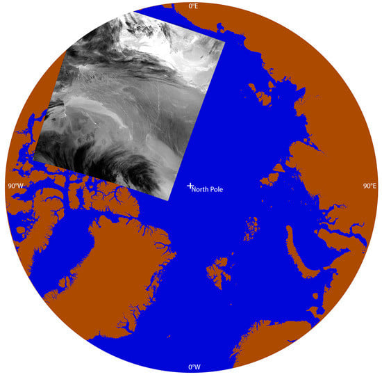
Figure 1.
MODIS-Terra 11 µm brightness temperature greyscale image from 15 February 2018 at 0545 UTC. Notice leads appear as bright (warm) features relative to the darker (colder) ice and clouds. The granule projection onto a 1 km Equal-Area Scalable Earth Grid version 2 (EASE2-Grid, [27]). The region shown is north of 65° N, with the North Pole in the center of the map.
2.1. Algorithm Description
The lead detection and characterization algorithm is divided into three steps. Figure 2 is a flowchart that summarizes the steps of this algorithm. Table 1 describes the different mask categories in the lead product, references will be given to the codes when describing the algorithm tests.
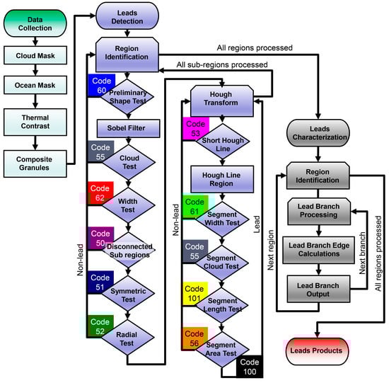
Figure 2.
Lead detection and characterization algorithm flowchart. Each color-coded column corresponds to a step in the process (step 1 in green, step 2 in blue, and step 3 in grey). Mask code numbers are used in NetCDF output files and the mask code colors form the color table used in the output imagery.

Table 1.
Summary of lead product codes and color table.
2.1.1. Step 1: Aggregate Imager Data, Identify Potential Leads
The Terra and Aqua MODIS 11 µm brightness temperature observations north of 65°N in each individual satellite overpass are remapped to a daily 1 km Equal-Area Scalable Earth Grid version 2 (EASE2-Grid, [27]) grid using a nearest neighbor approach. The brightness temperatures are derived from the Level1B Calibrated Radiances within the Collection 6 MxD021KM files [28,29] (“x” in the file name is “O” for Terra and “Y” for Aqua). For reference, Figure 1 shows an example granule using the EASE2-Grid. Land/Sea Mask within the Collection 6 MxD03 1km Geolocation files [30,31] is applied to exclude the land pixels. Cloud screening uses the standard MODIS cloud mask (MxD35; [25,32,33]). For our application, clear is defined when the cloud mask category is “confident clear”, with all other mask values as cloudy. To the nighttime overpasses (solar zenith angle greater than 85°), we apply a cloud removal filter developed by Fraser et al. [34] to remove false cloud detection over sea ice leads. Note that with no filtering the cloud mask flags likely leads as clouds, and the spatial filtering technique is used to reclassify these false clouds as clear, so that these features can be subjected to further lead detection testing.
Grid cells with cloud coverage less than a threshold of 25% in a 5 × 5 convolution kernel are reclassified as clear in Fraser et al. [34]. Using the example Terra overpass from 15 February 2018 at 0545 UTC, we test thresholds of 25% (green), 50% (blue) and 75% (red) of the spatial filter (Figure 3). Note that this image is not geolocated. The example is given to illustrate that filter performance is best for a threshold of 50% in a 5 × 5 pixel window (pixels in blue and green). When the threshold is low (pixels in green: 25% threshold), leads of larger size remain flagged as clouds. With a high threshold (red: 75%), degradation along cloud edges becomes prominent.
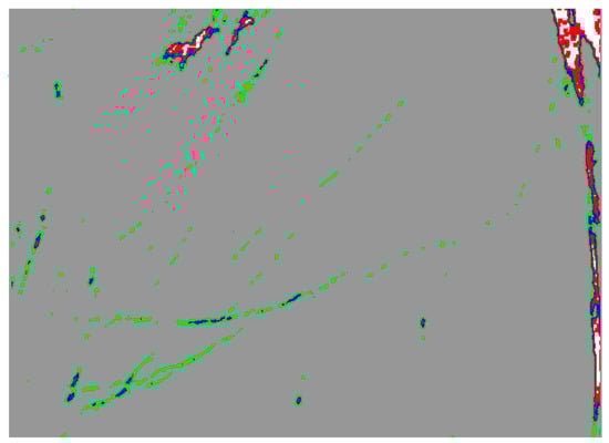
Figure 3.
Sample portion of MODIS-Terra cloud mask from 15 February 2018, at 0545 UTC. Gray areas are clear, unmodified clouds are white, and the original cloud mask defines clouds as all non-gray areas. A spatial filter is applied to remove false cloud detection over sea ice leads from the mask. In green (blue, red), 25% (50%, 75%) or less of the local mean is cloudy. The sample is a small portion of the same granule as Figure 1, the image is in the native, unnavigated satellite projection.
After the remapping, the algorithm detects possible sea ice lead pixels. A thermal contrast method is a primary component of possible lead detection. A pixel is identified as a potential sea ice lead if it has an 11 µm brightness temperature that is both 1.5 K greater than the mean, and greater than the standard deviation of the brightness temperature of its 25 by 25 pixel surrounding area. This approach is similar to what Willmes and Heinemann [16,17] described, except that we use the 11 µm brightness temperature instead of the derived surface temperature product. In addition, we constrain the MODIS scan angle to 30° within nadir, due to the degradation of spatial resolution at larger sensor viewing angles. The algorithm also assumes that a lead pixel will have a brightness temperature less than 271 K—the nominal freezing point of salt water (271.15 K is the freezing point of salt with salinity of 35 ppt). Due to the presence of open water or very thin sea ice, lead pixels will be below freezing but still warmer than the surrounding sea ice (where sea ice concentrations are 100%). At this point, the algorithm has identified potential leads; an example is shown in Figure 4. The algorithm detects most of the leads (black in Figure 4) that appeared as warm (white) features in the brightness temperature image (Figure 1).
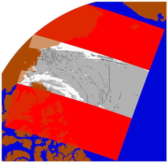
Figure 4.
MODIS-Terra potential lead mask from the single overpass at 0545 UTC on 15 February 2018 in the EASE2 projection. Potential leads are in black, clouds are white, land is brown, water not meeting the thermal contrast characteristics is grey, water outside of the image granule is blue, and the scan angle block-out is illustrated in red.
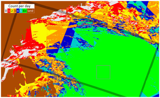
The procedure described above is applied to all Terra and Aqua overpasses on a given day. Rather than generating a composite of all possible sea ice leads pixels from all individual overpasses, our technique produces a map of the number of overpasses in a day where the thermal contrast tests are satisfied. Figure 5 shows a cropped section of a daily composite. Most of the areas where the thermal contrast test is satisfied in only one overpass (red) appear to be false leads - likely caused by short duration features such as clouds (cloud mask omission errors) or cloud shadows. The majority of the features that appear to be leads correspond to a color (shades other than gray and red in Figure 5) that indicates that the detection of the thermal feature occurred in multiple overpasses within the same day. A composite of the number of cloud-free overpasses at each location is also recorded (Figure 6). This map illustrates areas where sampling is limited or missing due to the scan angle constraints (over the pole and lower latitudes) or due to cloud cover. Lead detection is more likely in regions with frequent clear observations and less likely in regions with fewer overpasses or cloud contamination. The counts of clear, cloudy, and potential lead observations are provided in the output file. A user can infer higher confidence in detections when a potential lead (high thermal contrast) is detected in several overpasses, and lower confidence in regions with persistent clouds (a potential lead detection may be a cloud mask omission error).
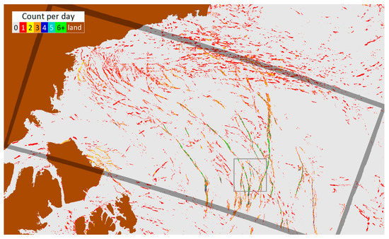
Figure 5.
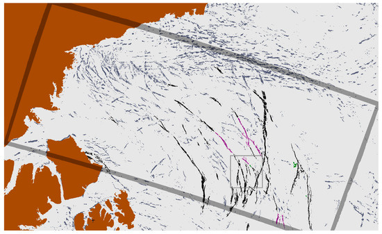
The number of overpasses when a potential lead is detected on 15 February 2018, a composite of all overpasses over the Beaufort Sea, remapped to the EASE2-Grid. The large boxed region corresponds with the location of the 0545 UTC granule shown in Figure 1. The small square is 200 km by 200 km and used for reference in Figure 7.
2.1.2. Step 2: Bulk Lead Detection
The daily composite map from Step 1—the composite of the number of times the thermal contrast suggests a potential lead may exist—will be referred to as the map of “potential leads”, this is represented in panel (a) in Figure 7 where a 200 by 200 km subset of the 15 February 2018 example is shown. In Step 2, the algorithm performs a number of geometric and image analysis tests on the mask of potential leads and builds a subset of positively identified bulk leads. The iterative process is depicted in Figure 7. The image analysis begins by identifying connected points in the potential lead mask (Figure 7, panel b), where each continuous object has a unique color. A rough estimate of the object width is used to test if an object is a non-lead open water feature (e.g., a polynya). This width is defined as the object area divided by the square root of the sum of the square of the span of the object in the x and y directions (in the equal area grid), as the line from point 1 to 4 in panel c. The region is considered as open water and no further lead processing performed if the width estimate is greater than 60 km (code 60 in Table 1). The lead detection algorithm next rejects potential lead regions that contain only one or two pixels as being too small. Applying these preliminary tests reduces algorithm runtime time by removing some features before applying computational expensive image analysis techniques.
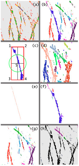
Figure 7.
Example application of lead detection. (a) the number of times a potential lead detected from a small section (gray square) in Figure 5. (b) the region divided into connected objects, each continuous object having a different color. (c) the largest continuous object from panel (b) being subjected to additional testing. (d) the result after applying the Sobel filter with each continuous object having a unique color. (e) the longest Hough Transform line segment. (f) a potential lead cluster, with discontinuous object being connected in the Sobel filter version of the object in panel (d). (g) a new iteration with the object from (f) removed from (b). (h) the final results; refer to Table 1 for the product color table.
A Sobel image filter [35] is applied to the mask of the remaining potential leads, resulting in each continuous object being assigned a unique color (Figure 7, panel d). The Sobel image filter is an edge detection image-processing tool. For lead detection, the advantage of using the Sobel filter is that it can connect discontinuous features. The width of a lead may fluctuate above and below the nominal resolution of the MODIS imager along the path of the lead. The result would be a single object (lead) that appears as a series of discontinuous (sub-resolution) points in the native imagery. Applying the Sobel filter to the binary mask of the number of times a potential lead is detected, related groups of discontinuous objects are combined into a single continuous object that is subjected to further lead testing.
Cloud artifacts (cloud shadows, cloud mask omission errors, and cloud edges) can cause thermal contrast features that look similar to the thermal contrast from a lead. However, cloud artifacts tend to be short-lived either because the cloud moves, the satellite and/or solar view angle changes, or cloud mask omission errors might not persist in subsequent observations. Therefore, the algorithm contains a test that checks the number of overpass the thermal contrast conditions have been satisfied. For the area of each continuous potential lead feature, a test requires that more than 90% of the observed area within a lead must occur in two or more overpasses within a day. This test (Table 1, code 55) removes features that are most likely cloud contamination (cloud mask omission error) from becoming detected leads, but still allows detection of a lead that is changing (growing, shrinking, or moving) over the course of a day (providing that no more than 10% of the lead area is detected in only one overpass). This 90%/10% threshold was derived empirically by examining several test scenes over several days.
The potential lead undergoes additional geometric testing. First, the original mask (panel b of Figure 7) is compared against the Sobel filtered mask (panel d of Figure 7) to form panel (f) of Figure 7. The number of disconnected features in the original mask (number of colors in panel (f)) are counted that correspond to the single potential lead object region from the Sobel filter (coral color object in panel (d)). A non-lead flag (code 50) is assigned if an object has too many sub-regions or if too much of the object area is made up of small (less than 5 km2) sub-regions. There is also a test for the object symmetry to test if the object area is too symmetrical (Table 1, code 51), it fails to be a lead. The symmetry test defines four equal-sized quadrants that encompass the test object, black rectangles in panel (c) of Figure 7 and an object fails to be a lead if each of the quadrants contain between 17%-33% of the object area. Similarly, the radial test defines a green circle in panel (c) of Figure 7 centered on the center of the rectangle (point 5) that encompasses the object undergoing analysis. The radius of the circle is half of the average of the length and width of the rectangle that encompasses the object. For the radial test, the number of object points that overlap with the edge of test circle versus the number of points where the object does not overlap with edge of the test circle are calculated. The test object fails to be a lead if more than 50% of the circumference of the test circle overlaps with the test object (Table 1, code 52). The geometric thresholds described in this paragraph were all established empirically by testing a range of values on the synthetic dataset and examining several test scenes over several days.
After passing the preliminary shape tests, the next step is to identify linear features. Leads can be assumed to be polylines and for this reason a Hough Transform [36] is used to locate linear features in imagery. The Hough Transform identifies the longest linear feature within the mask of the number of times a potential lead has been detected. For example, the transform is applied to Figure 7, panel d, and the longest resulting line is shown in panel e. Processing iterations of the longest remaining line continue in a loop until the longest Hough line has three points or less (regions with less than three points are too short and flagged as a non-lead, code 53, Table 1). If the Hough line (panel f) is longer than three points, then a sub-region is defined as all continuous points connected with the longest Hough line segment (panel c). This sub-region undergoes additional testing. The length of the longest line segment within the sub-region is compared against the length of the Hough line segment (lengths of panel c points 1 to 4 compared against panel e). If the sub-region area is greater than 2 points, a few final tests classify the region as a lead or non-lead (Table 1, codes 61, 55, 101, and 56). Processing the largest remaining lead sub-region, each potential lead object is processed until no more valid Hough line segments in the region are found. Or, using the illustration, panel f is removed from panel b to form panel g, the iterative process continues with panel g replacing panel b until the only remaining features contain less than 2 continuous points (features too small to identify a linear features).
2.1.3. Step 3: Lead Branch Characterization
The last step in the processing determines lead characterization. Prior to this step a lead has been defined as a bulk object, or a continuous feature that has high thermal contrast and has passed a series of image processing tests. The previous tests derive characteristics of individual segments or branches that are within the larger, and potentially complex, multifaceted object. The input for this step is the bulk lead mask, described in previous sections. A morphological erosion function (3 by 3 square array) removes the edges from lead object regions. By essentially removing the thinnest segments from a lead, the result is a mask that contains more disconnected regions than the original mask; these discontinuous sub-regions are defined as lead branch segments. An example is shown in Figure 8. In the example, panel e represents a bulk lead object detected in Step 2, each color in panel g represents a lead branch segment. Each bulk and branch object are represented in separate text output files, the object (bulk lead or branch segment) area, length, width, orientation, and coordinates for a start and end point are listed in the respective text output file.
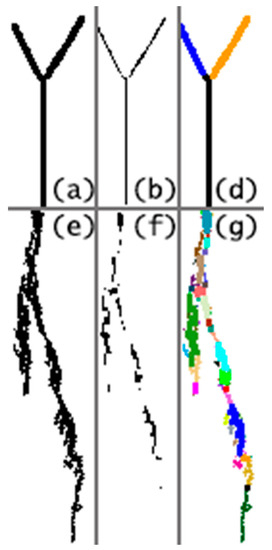
Figure 8.
Left objects (a) and (e) show bulk lead; the eroded branched lead is in the center panels (b) and (f); and the right panels (d) and (g) show the restored lead with each branch shown as a different color. The top row is an idealized synthetic lead, the bottom row is an example lead detected on 15 February 2018.
The branch processing loop starts by identifying the remaining branch with the largest area. For each lead branch, the first step is to isolate the edge or outline of the region. The start and end point of the lead branch are identified by finding the set of coordinates that are the furthest distance apart from each other. The great circle distance and azimuth angle are calculated between the start and end points. The segment width is another derived characteristic, found by dividing the segment area by the great circle distance. The sea-basin code for start and end points of the branch is recorded to more readily locate leads as a function of sea, while noting that some leads may span across sea boundaries.
An output text file describes lead characteristics for every (branch or bulk) lead identified in the raster mask. These files serve two purposes: the text file can provide lead location information to users with low bandwidth capabilities and the files provide the metadata of lead characteristics. For each lead branch, the start and end coordinates (x, y, longitude, and latitude), length, azimuth, width area, and the sea code that corresponds to the start and end point of the branch.
2.2. Output Format
The leads product is available online (ftp://frostbite.ssec.wisc.edu). A navigation file is provided (ftp://frostbite.ssec.wisc.edu/latlon.nc) with the latitude and longitude for each point of the EASE2-Grid. The leads products are arranged in subdirectories by year. The daily product file format is NetCDF. Within the NetCDF file are four different masks, the leads mask and three ancillary arrays. The leads mask is a coded field indicating lead detection (code 100) and rejection codes (see Table 1). The ancillary data includes a cloud mask that reports the number of overpasses at each location that was cloudy (or rejected from processing due to the scan angle block-out), a coverage array that reports the number of cloud-free overpasses, and a potential lead array reports the number of overpasses a potential lead was detected. Two daily text files are also available, one for the bulk lead objects and the other for lead branches. These text files report the coordinates of the start and end point of the lead as well as characteristics such as length (great circle distance from start and end point), azimuth angle, object area, and width (derived as area divided by length). Readme files are included on the ftp site to help describe each output field.
3. Results
This paper presents a technical description of the algorithm. A later publication is anticipated with a greater focus on the results and trend analyisis. A synthetic test case and a real-world test case are presented as an assessment of the algorithm. The synthetic case is designed to assist in the development of the algorithm; tests and thresholds are set by testing performance against the synthetic scene as well as real-world case studies. Comparisons are presented against products from previously published lead detection technique. Annual lead area coverage maps over the Arctic are also included.
3.1. Synthetic Test
A synthetic test scene is used to assess algorithm performance. Using this synthetic data, in combination with test cases with real data, many of the algorithm thresholds were tested and defined. The test scene contains lead-like features as well as features that do not resemble leads and should fail a lead detection algorithm. Figure 9 shows the test scene with results from the algorithm. Black represents areas that pass as lead detections; other colors represent areas that the algorithm rejects object as a lead for reasons shown in Table 1. The top three quarters of the bulk objects resemble leads, the bottom quarter of the image represents features that were designed to not resemble leads. Several of the algorithm tests were designed and thresholds adjusted based on the detection/rejection performance with the synthetic dataset. Detection is successful for the continuous linear features in the test scene (except for some lines that are too straight and too thin). Detection failures occur sometimes when breaks in a line segment are too small or too wide. This testing provides us with the confidence to apply the algorithm to satellite imagery scenes.
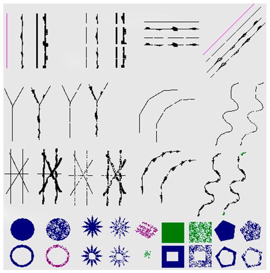
Figure 9.
Synthetic algorithm test scenes and test results. Objects that pass lead detection are in black; other colors represent potential leads that fail one of the tests. Refer to Table 1 for mask code colors. Not all categories are represented in this example.
3.2. Case Studies
An example MODIS product result from 15 February 2018 is shown in Figure 10. This is the same case illustrated in previous figures. One image granule is shown on a map in Figure 1 and the potential leads identified in that single overpass are mapped in Figure 4. The majority of potential lead features found in only in one overpass (red in Figure 5) are rejected from the final leads product mask. A more detailed description of the algorithm for the small gray square was presented in Figure 7. Notice that some of features that look like leads are rejected sometimes; these objects have complex shapes that fail one of the identification tests. Also, for cases where there was only one clear overpass, a potential lead will fail our detection technique.
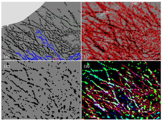
For comparison against other lead detection methods, a second case study from 3 March 2009 is presented in Figure 11 and Figure 12. For a general overview, Figure 11 shows the entire polar domain. Figure 12 highlights some details enlarged on a small box region in Figure 11. Our leads products are shown in panels (A) and (a); refer to Table 1 for the color table of leads (black) and potential leads that fail the linear classification technique. MODIS lead detections from Willmes and Heinemann product [37] are shown in black and the artifact (high uncertainty) category is colored red in panels (B) and (b); lead detections from Röhrs and Kaleschke [18] (and Röhrs et al. [19]) using AMSR-E [38] are also shown in black in panels (C) and (c). These products have been remapped and resampled with a nearest neighbor technique to match the same projection and 1km resolution as our product. To highlight the product similarities and differences, the fourth panel (D) and (d) is an RGB composite of the three products. With leads from our product in the red channel, the Willmes and Heinemann product is in the blue channel, and the Röhrs AMSR-E product is in the green channel. Notice that where all three products detect a lead, the pixel is colored white; yellow, cyan, and purple result when two of the three products detect a lead. As expected, the advantage of AMSR-E is the ability to detect leads in cloud regions, the drawback is that it only detects relatively large leads and tends to over-represent lead width due to the coarser spatial resolution (see the Discussion section). The Willmes and Heinemann technique detects more leads than our product (Figure 11 and Figure 12); many features Willmes and Heinemann classify as leads fail our tests that try to identify linear features.
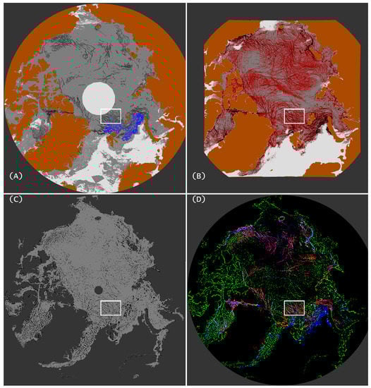
Figure 11.
Example case from 3 March 2009. Our leads product in panel (A), refer to Table 1 for the leads color table. Leads detected from Willmes and Heinemann product [37] are shown in black and the artifact (high uncertainty) category is in red in panel (B). AMSR-E [38] leads are in black in panel (C). An RGB composite is shown in panel (D), here, our leads are in red, Willmes and Heinemann leads in blue, and AMSR-E in green. A 650 km by 500 km region (white box) is enlarged in Figure 12.
3.3. Lead Timeseries
The lead algorithm is applied to Terra and Aqua MODIS observations for the period January through April for the years 2003–2018. The reasons for limiting the study period to January through April is discussed later in the discussion section. An overview map of annual lead frequency (number of days with a lead detection from January through April) is presented in Figure 13 and Figure 14. A daily animation of lead detections is available in Supplemental Materials S1. The variations of sea ice lead frequency from region-to-region and year-to-year is a topic to be addressed in future work.
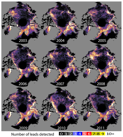
Figure 13.
Lead frequency map by year 2003–2011. Color coded legend is at bottom of the figure represents number of days with a lead detected between January through April.
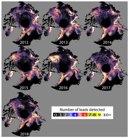
Figure 14.
Lead frequency map by year 2012–2018. Color coded legend is at bottom of the figure represents number of days with a lead detected between January through April.
A comparison of the time-series of our results and the Willmes and Heinemann [37] product is presented in Table 2. The statistics are arranged in rows by year, with all years combined in the bottom row. The second through fourth columns give statistics independent of the spatial domain of other product. The remaining three columns give statistics from the subset of the domain where both products had cloud-free coverage. The area that we classify as potential leads (defined as a percentage of area with a positively identified lead or potential lead, divided by coverage area) is in better agreement with what Willmes and Heinemann classify as leads than the final lead classification (“leads”), as the linear identification techniques that our algorithm employs results in fewer positively identified leads. Comparing the statistics with and without the overlapping coverage of both products, the results are similar. The statistics tend to be only a fraction of a percent higher for the subset where both products have coverage over the same domain.
Table 2.
Annual statistical difference of leads products. Area is reported as a percentage of leads area divided by coverage area. Positively identified leads and potential leads are compared against Willmes and Heinemann [37] leads (artifact category is not included), which is only available for 2003–2015. The left set of columns are for each product independently. On the right, the domains are limited to only the subset where both products have coverage.
Figure 15 is a map of the Arctic divided into seas as defined by Wang and Key [39]. Figure 16 shows the orientation, as an azimuth angle, of leads in the 10 seas for each year in the period 2003–2018. An azimuth of 0 degrees is north-south; azimuth is reported as degrees east of north (or degrees moving clockwise) with a range of 0–180. The distribution of azimuth angles that define orientation of the leads varies for each sea but is relatively consistent for all years within any given sea. Figure 17 shows the relative frequency of lead widths, areas, and lengths for individual years. The aggregate of all seas is used for this series of plots. Lead branch segments (described in algorithm Step 3) are on the top row and bulk lead objects (described in algorithm Step 2) are on the bottom row. Notice that the scales are different between the rows where the branches are smaller than the bulk objects; one or multiple branch segments comprise a bulk lead object. The intent here is to showcase the capabilities of the algorithm. The small inter-annual variability and analysis of the patterns in lead characteristics will be focuses of future research.
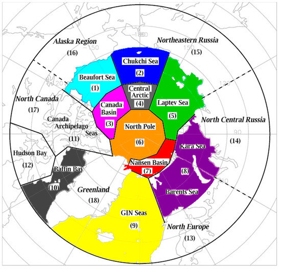
Figure 15.
Color-coded Arctic map with each region assigned a sea name and number.
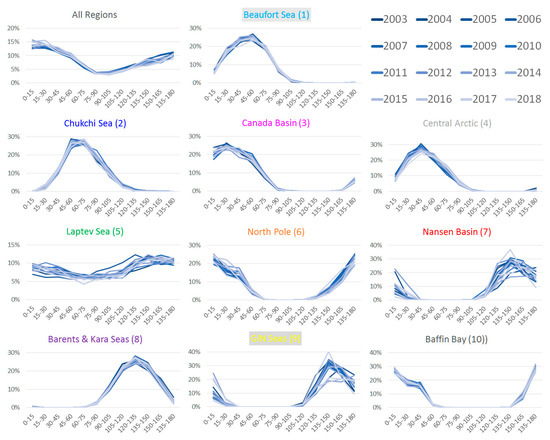
Figure 16.
Sea ice lead azimuth angle distributions in 10 seas (Figure 15), color-coded for years 2003–2018.
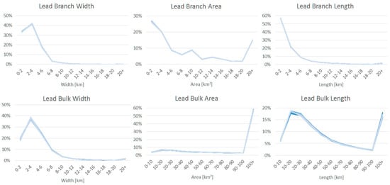
Figure 17.
Relative frequency of lead widths, areas, and lengths with the same color code as Figure 16 for 2003–2018. Here, an aggregate of all seas is shown for the individual lead branch segments on the top row and for overall lead objects on the bottom row, the distinction being that a lead object is made up of one or multiple branch segments.
4. Discussion
The design philosophy of our algorithm is to minimize the errors of commission; i.e., to minimize overestimation of leads. As presented in Table 2, the area classified as potential leads is in better agreement with the Willmes and Heinemann [37] leads area than our positively identified leads. Quantitative results are presented annually; qualitative comparisons of an example day are shown in Figure 11 and Figure 12. The quantitative results from the day of the case study are similar to the annual results (not shown). Although both products are derived from the same satellite, there are some differences in the domain. Willmes and Heinemann [16,17] does not extend as far south however, our algorithm limits the view angle (creating a coverage gap at the pole). Cloud coverage results in some difference as well. We apply a cloud screening technique that allows for some lead retrievals in areas where the ice surface temperature is not retrieved due to cloud, and therefore Willmes and Heinemann [16,17] cannot process a location for leads. Some of these differences are visible in the case study shown in Figure 11.
Furthermore, our positively identified lead area is significantly smaller. When comparing statistics where both have cloud-free coverage, our technique finds leads in approximately 3% of the domain compared with approximately 10% of the Willmes and Heinemann domain. Some of the differences can be attributed to resampling of the Willmes and Heinemann [37] product; the nominal native resolution of that product is 2 km resolution while our product resolution is 1 km. Using the coarser resolution, the contribution of sub-resolution leads may overestimate the total lead area. We are able to achieve the finer resolution by limiting the scan angle to 30°, though the trade-off is a coverage gap over the pole (north of approximately 81°N). The effects of sensor resolution on lead characteristics were examined in [11,12,40]. Using Landsat Multi-Spectral Scanner 80 m data degraded to lower resolutions, Key et al. [12] found that (a) while the manner in which widths of individual leads changes with increasing pixel size is highly variable, the mean lead width over an image changes in a more predictable way. For example, a mean lead width of 400 m derived from data with a 200 m pixel may “grow” to a mean width of 800–1000 m with a 700 m pixel (Figure 6 in [12]). (b) The change in total lead area with increasing pixel size is generally exponential. (c) Leads narrower than approximately 250 m disappear as the resolution of Landsat images is degraded to 320 and 640 m. (d) Lead orientations change if they are anisotropic (i.e., have a preferred orientation), but do not change substantially if they are isotropic. The actual effect of pixel size depends in part upon the temperature or reflectance contrast between a lead and the surrounding ice; see [12] for a quantification of the combined effect.
The difference in lead area is also a result of the different linear identification techniques that our algorithm employs. If there are applications that are less sensitive to commission error and more sensitive to omission error, users can refer back to Table 1 for a summary of lead rejection categories and they may choose to include some rejection categories in addition to our positively identified leads category. A polynya is an example of an ice feature with the thermal signature of leads, but it is irregularly shaped. [41] Our algorithm is tuned towards identifying leads as linear features within the sea ice pack.
We use Level1B 11 μm brightness temperatures [28,29] rather than the MODIS MxD29 ice surface temperature product [42,43,44]. The MODIS noise-equivalent temperature difference is 0.05 K at 11 μm channel, which is sufficiently accurate for lead detection. There is, of course, a strong correlation between ice surface temperature and the 11 μm brightness temperature. Also, the actual surface temperature is less important than the contrast in temperature. Leads become undetectable when the thermal contrast between leads and surrounding ice pack is small (e.g., less than 1.5 K, although the local spatial variability is also a factor, as described earlier). The primary cause of thermal contrast in the Arctic winter would be leads—the contrast between solid ice and either open water, ice and water mixed, or thin ice. In warmer seasons the contrast between ice temperature and water temperature becomes smaller. Detection capabilities decreases as the surface temperature increases. In summary, the temperature contrast becomes small as ice becomes thicker within a lead or when the surface temperature approaches the melting point of ice in the case of an unfrozen lead.
We agree with the findings of Fraser et al. [34] that cloud masks often misidentify leads as clouds. We are able to employ a similar cloud clearing method to reclassify false cloud detections as clear and detect leads using the 11 μm brightness temperature. It would not be possible to detect leads using the sea ice temperature in these locations because the sea ice temperature product would fail to provide a temperature retrieval in these areas flagged as cloudy. Another area of investigation was to use an ice concentration product as the basis for identifying potential leads, but we found that much like ice surface temperature products, cloud product omission errors (associated with leads) often prevented ice concentration retrievals just as clouds also prevent ice surface temperature retrievals.
Clouds present several obstacles in lead detection. The infrared thermal signature of clouds is often similar to that of leads, which is why cloud detection algorithms often errantly flag leads as clouds. Polar cloud detection in the winter is difficult; cloud detection algorithms are designed to detect cold and highly reflective features, which happen to also be characteristics of sea ice. Further, cloud mask performance is in general better during the day—when reflective bands contribute to better performance of cloud detection algorithms—but the polar region is predominately dark during the winter. Also, clouds in the polar winter are commonly warmer than the surface. Cloud detection algorithms use ancillary data to try to identify in advance where snow or ice may exist at the surface in an attempt to detect clouds over snow or ice. The problem with this technique is that the ancillary data might not accurately reflect the actual conditions; the product may be observation based and reflective of past conditions that may be obsolete or based on a forecast that is not reflective of current conditions. Also, the resolution of the snow/ice mask may be too coarse resolution to account for narrow features like leads.
One of the weaknesses of the algorithm is that it was not designed to work in the summer months. The thermal contrast between leads and the surrounding ice would be very different and the surface can be more complex. Melt ponds, for example, may appear in the summer and these could potentially fool the algorithm. When the ice surface temperature approaches the water temperature, the algorithm would not detect thermal contrast and therefore not detect leads. Persistent cloud coverage in the warmer months is another factor for the limited period of coverage. The January through April time period was chosen because this is generally the best season for lead detection and it is consistent with the season provided by Willmes and Heinemann [37].
One of the advantages of the polar region is the frequent coverage from polar satellites. One of the assumptions of the algorithm is that most locations in the domain will have been covered by multiple satellite overpasses. As illustrated in Figure 6, most locations have over six overpasses per day, though cloud coverage will limit the number of overpasses where lead detection is possible.
In addition to frequent repeating coverage, another assumption the algorithm makes is that leads will be stationary or slow moving in order to satisfy the requirement that a lead must be detected in multiple overpasses. To account for lead movement there is a requirement that 90% of the lead area must be detected in multiple overpasses. A fast-moving lead could fail to meet these conditions; however, the alternative has drawbacks. If a lead is moving quickly such that it appears in different locations throughout the day, a daily composite of lead area could over-report lead area because the fast-moving lead area would be counted towards the daily area in each location it was detected (versus stationary leads that would only contribute towards the daily area once). We believe the smearing effect from slow moving leads that could artificially inflate the lead width and area is more acceptable than considering each detection of a fast-moving lead as a contribution towards the daily lead area. We also believe that repeat detections are important to establishing confidence in a lead detection. The type of phenomena that would produce a thermal contrast signature similar to that of leads would either be a broken ice feature like a lead or else related to a cloud. Cloud edges, cloud shadows, and cloud mask omission errors could all produce a thermal contrast signature similar to a lead. These cloud related features are more likely to be short lived; we would expect viewing geometry and cloud movement to change overpass-to-overpass and make the reoccurrence of false lead signatures less likely than for repeat observations of a real lead. Establishing a confidence parameter would be a non-trivial undertaking. Providing the number of times a potential lead was detected can be used subjectively to help establish user confidence in lead detections. In future work a confidence may be established based on observation frequency as well as other factors such as making an attempt to track a previously detected lead or perhaps quantifying the thermal contrast signature into a confidence parameter.
5. Conclusions
This paper describes an algorithm to detect sea ice leads (fractures) over the Arctic using measurements from MODIS on the Terra and Aqua satellites. We describe the algorithm and demonstrate results by applying the algorithm over the entire MODIS Aqua/Terra period, 2003–2018, for the winter and early spring months of January–April. The algorithm consists of three main steps. The first step makes a 1-km grid composite of the potential leads based on the thermal contrast in the satellite infrared window data over the Arctic Ocean. The second step defines lead objects using a series of image analysis techniques to identify pixels that may have spatial characteristics of leads. In the third and final step, lead objects are broken into smaller individual branches and the characteristics of each branch of a potentially multi-faceted lead are calculated. This step also determines the area, length, width and orientation of the lead. The results of this algorithm are compared with the products from Willmes and Heinemann [37] who also use MODIS but employ a different methodology.
Cloud coverage constrains lead detection, optically thick clouds in particular, thus an infrared algorithm for lead detection requires an accurate cloud mask. Unfortunately, the most difficult conditions for automated cloud identification techniques—nighttime darkness, bright surfaces, and cold surfaces—are also the most prevalent conditions in the Arctic winter. Also, the thermal contrast and shape of cloud edges and cloud shadows often have a similar shape and temperature contrast as lead. Passive microwave observations overcome many problems associated with cloudy conditions but have a larger footprint. Combining collocated microwave and imager observations may be the best approach to determining changing lead characteristics in the Arctic.
Instrument resolution is another limiting factor. By limiting the sensor scan angle we are able to keep our observation resolution at a relatively consistent 1 km. We did not attempt to define the minimum detectable lead size; it would be a function of the lead size, water temperature (and sea ice concentration) within the leads, and the temperature of the surrounding sea ice.
Future work will explore the relationship between cloud cover and the lead detection, trends in lead length and width, relationships between lead azimuth angle and anomalies in wind and ocean currents, and relationships between changes in lead properties and sea ice thickness. Application of the algorithm indicates that the annual variation in lead coverage is large, both spatially and temporally. The algorithm will be adapted to the Visible Infrared Imaging Radiometer Suite (VIIRS), which has more consistent spatial resolution of 375 m across the entire 11 μm swath. With a wider swath than MODIS, the two-satellite system of NOAA-20 and the Suomi National Polar-orbiting Partnership satellites will be able to provide even greater coverage than has been available with MODIS.
Supplementary Materials
The following are available online at https://youtu.be/r7ax0uJtZX0, Video S1: 2003–2018 Daily Leads Detections.
Author Contributions
Conceptualization, J.P.H., S.A.A., Y.L. and J.R.K.; Data curation J.P.H. and Y.L.; Funding acquisition, S.A.A.; Investigation, J.P.H.; Methodology, J.P.H. and J.R.K.; Project administration, S.A.A.; Resources, J.R.K.; Software, J.P.H., Y.L. and J.R.K.; Supervision, S.A.A.; Validation, J.P.H. and Y.L.; Writing—original draft, J.P.H.; Writing—review & editing, J.P.H., S.A.A., Y.L. and J.R.K.
Funding
This research was funded by NASA, grant number NNX14AJ42G and 80NSSC18K0786.
Acknowledgments
The Aqua and Terra MODIS datasets were acquired from the Level-1 and Atmosphere Archive & Distribution System (LAADS) Distributed Active Archive Center (DAAC), located in the Goddard Space Flight Center in Greenbelt, Maryland (https://ladsweb.nascom.nasa.gov/). The Willmes and Heinemann MODIS leads product dataset acquired from https://doi.pangaea.de/10.1594/PANGAEA.854411. The Röhrs et al. AMSR-E dataset acquired from https://icdc.cen.uni-hamburg.de/1/daten/cryosphere/lead-area-fraction-amsre.html. The views, opinions, and findings contained in this report are those of the author(s) and should not be construed as an official National Oceanic and Atmospheric Administration or U.S. Government position, policy, or decision.
Conflicts of Interest
The authors declare no conflict of interest.
References
- Smith, S.D.; Muench, R.D.; Pease, C.H. Polynyas and leads: An overview of physical processes and environment. J. Geophys. Res. Oceans 1990, 95, 9461–9479. [Google Scholar] [CrossRef]
- Alam, A.; Curry, J. Lead-induced atmospheric circulations. J. Geophys. Res. Oceans 1995, 100, 4643–4651. [Google Scholar] [CrossRef]
- Maykut, G.A. Energy exchange over young sea ice in the central arctic. J. Geophys. Res. Oceans 1978, 83, 3646–3658. [Google Scholar] [CrossRef]
- Lüpkes, C.; Vihma, T.; Birnbaum, G.; Wacker, U. Influence of leads in sea ice on the temperature of the atmospheric boundary layer during polar night. Geophys. Res. Lett. 2008, 35. [Google Scholar] [CrossRef]
- Douglas, T.; Sturm, M.; Simpson, W.; Brooks, S.; Lindberg, S.; Perovich, D. Elevated mercury measured in snow and frost flowers near arctic sea ice leads. Geophys. Res. Lett. 2005, 32. [Google Scholar] [CrossRef]
- Steiner, N.; Lee, W.; Christian, J. Enhanced gas fluxes in small sea ice leads and cracks: Effects on CO2 exchange and ocean acidification. J. Geophys. Res. Oceans 2013, 118, 1195–1205. [Google Scholar] [CrossRef]
- Wadhams, P.; Davis, N.R. Further evidence of ice thinning in the Arctic Ocean. Geophys. Res. Lett. 2000, 27, 3973–3975. [Google Scholar] [CrossRef]
- Vaughan, D.G.; Comiso, J.C.; Allison, I.; Carrasco, J.; Kaser, G.; Kwok, R.; Mote, P.; Murray, T.; Paul, F.; Ren, J. Observations: Cryosphere. Clim. Chang. 2013, 2103, 317–382. [Google Scholar]
- Laxon, S.W.; Giles, K.A.; Ridout, A.L.; Wingham, D.J.; Willatt, R.; Cullen, R.; Kwok, R.; Schweiger, A.; Zhang, J.; Haas, C. Cryosat-2 estimates of arctic sea ice thickness and volume. Geophys. Res. Lett. 2013, 40, 732–737. [Google Scholar] [CrossRef]
- Rampal, P.; Weiss, J.; Marsan, D. Positive trend in the mean speed and deformation rate of arctic sea ice, 1979–2007. J. Geophys. Res. Oceans 2009, 114. [Google Scholar] [CrossRef]
- Key, J.; Stone, R.; Maslanik, J.; Ellefsen, E. The detectability of sea-ice leads in satellite data as a function of atmospheric conditions and measurement scale. Ann. Glaciol. 1993, 17, 227–232. [Google Scholar] [CrossRef]
- Key, J.; Maslanik, J.; Ellefsen, E. The effects of sensor field-of-view on the geometrical characteristics of sea ice leads and implications for large-area heat flux estimates. Remote Sens. Environ. 1994, 48, 347–357. [Google Scholar] [CrossRef]
- Lindsay, R.; Rothrock, D. Arctic sea ice leads from advanced very high resolution radiometer images. J. Geophys. Res. Oceans 1995, 100, 4533–4544. [Google Scholar] [CrossRef]
- Miles, M.W.; Barry, R.G. A 5-year satellite climatology of winter sea ice leads in the western arctic. J. Geophys. Res. Oceans 1998, 103, 21723–21734. [Google Scholar] [CrossRef]
- Drüe, C.; Heinemann, G. High-resolution maps of the sea-ice concentration from MODIS satellite data. Geophys. Res. Lett. 2004, 31. [Google Scholar] [CrossRef]
- Willmes, S.; Heinemann, G. Pan-arctic lead detection from MODIS thermal infrared imagery. Ann. Glaciol. 2015, 56, 29–37. [Google Scholar] [CrossRef]
- Willmes, S.; Heinemann, G. Sea-ice wintertime lead frequencies and regional characteristics in the arctic, 2003–2015. Remote Sens. 2015, 8, 4. [Google Scholar] [CrossRef]
- Röhrs, J.; Kaleschke, L. An algorithm to detect sea ice leads by using AMSR-E passive microwave imagery. Cryosphere 2012, 6, 343–352. [Google Scholar] [CrossRef]
- Röhrs, J.; Kaleschke, L.; Bröhan, D.; Siligam, P.K. Corrigendum to “An algorithm to detect sea ice leads by using amsr-e passive microwave imagery.”. Cryosphere 2012, 6, 365. [Google Scholar]
- Bröhan, D.; Kaleschke, L. A nine-year climatology of arctic sea ice lead orientation and frequency from AMSR-E. Remote Sens. 2014, 6, 1451–1475. [Google Scholar] [CrossRef]
- Ivanova, N.; Rampal, P.; Bouillon, S. Error assessment of satellite-derived lead fraction in the arctic. Cryosphere 2016, 10, 585–595. [Google Scholar] [CrossRef]
- Murashkin, D.; Spreen, G.; Huntemann, M.; Dierking, W. Method for detection of leads from Sentinel-1 SAR images. Ann. Glaciol. 2018, 59, 124–136. [Google Scholar] [CrossRef]
- Zakharova, E.A.; Fleury, S.; Guerreiro, K.; Willmes, S.; Remy, F.; Kouraev, A.V.; Heinemann, G. Sea ice leads detection using Saral/Altika altimeter. Mar. Geod. 2015, 38, 522–533. [Google Scholar] [CrossRef]
- Wernecke, A.; Kaleschke, L. Lead detection in arctic sea ice from Cryosat-2: Quality assessment, lead area fraction and width distribution. Cryosphere 2015, 9, 1955–1968. [Google Scholar] [CrossRef]
- Frey, R.A.; Ackerman, S.A.; Liu, Y.; Strabala, K.I.; Zhang, H.; Key, J.R.; Wang, X. Cloud detection with MODIS. Part i: Improvements in the MODIS cloud mask for Collection 5. J. Atmos. Ocean. Technol. 2008, 25, 1057–1072. [Google Scholar] [CrossRef]
- Liu, Y.; Key, J.R.; Frey, R.A.; Ackerman, S.A.; Menzel, W.P. Nighttime polar cloud detection with MODIS. Remote Sens. Environ. 2004, 92, 181–194. [Google Scholar] [CrossRef]
- Brodzik, M.J. EASE-Grid: A versatile set of equal-area projections and grids. In Discrete Global Grids; Goodchild, M., Knowles, K.W., Eds.; National Center for Geographic Information & Analysis: Santa Barbara, CA, USA, 2002. [Google Scholar]
- MODIS Science Data Support Team (SDST). Available online: http://dx.doi.org/10.5067/MODIS/MOD021KM.006 (accessed on 29 January 2019).
- MODIS Science Data Support Team (SDST). Available online: http://dx.doi.org/10.5067/MODIS/MYD021KM.006 (accessed on 29 January 2019).
- MODIS Science Data Support Team (SDST). Available online: http://dx.doi.org/10.5067/MODIS/MYD03.006 (accessed on 29 January 2019).
- MODIS Science Data Support Team (SDST). Available online: http://dx.doi.org/10.5067/MODIS/MOD03.006 (accessed on 29 January 2019).
- Ackerman, S.A.; Strabala, K.I.; Menzel, W.P.; Frey, R.A.; Moeller, C.C.; Gumley, L.E. Discriminating clear sky from clouds with MODIS. J. Geophys. Res. Atmos. 1998, 103, 32141–32157. [Google Scholar] [CrossRef]
- Baum, B.A. Modis cloud-top property refinements for collection 6. J. Appl. Meteorol. Climatol. 2012, 51, 1145. [Google Scholar] [CrossRef]
- Fraser, A.D.; Massom, R.A.; Michael, K.J. A method for compositing polar MODIS satellite images to remove cloud cover for landfast sea-ice detection. IEEE Trans. Geosci. Remote Sens. 2009, 47, 3272–3282. [Google Scholar] [CrossRef]
- Sobel, I. Camera Models and Perception. Ph.D. Thesis, California: Artificial Intelligence Lab. Stanford University, Stanford, CA, USA, 1970. [Google Scholar]
- Ballard, D.H. Generalizing the Hough transform to detect arbitrary shapes. Pattern Recognit. 1981, 13, 111–122. [Google Scholar] [CrossRef]
- Willmes, S.; Heinemann, G. Daily pan-arctic sea-ice lead maps for 2003–2015, with links to maps in netCDF format. In Supplement to: Willmes, S; Heinemann, G (2015): Sea-Ice Wintertime Lead Frequencies and Regional Characteristics in the Arctic, 2003–2015. Remote Sens. 2015, 8, 4. [Google Scholar] [CrossRef]
- Integrated Climate Date Center. AMSR-E Lead Area Fraction for the Arctic, 3 March 2009, Ed; University of Hamburg: Hamburg, Germany.
- Wang, X.; Key, J.R. Arctic surface, cloud, and radiation properties based on the AVHRR Polar Pathfinder dataset. Part I: Spatial and temporal characteristics. J. Clim. 2005, 18, 2558–2574. [Google Scholar] [CrossRef]
- Key, J.R. The area coverage of geophysical fields as a function of sensor field-of-view. Remote Sens. Environ. 1994, 48, 339–346. [Google Scholar] [CrossRef]
- Paul, S.; Willmes, S.; Heinemann, G. Long-term coastal-polynya dynamics in the southern Weddell Sea from MODIS thermal-infrared imagery. Cryosphere 2015, 9, 2027–2041. [Google Scholar] [CrossRef]
- Hall, D.K.; Riggs, G.A.; Salomonson, V.V.; Barton, J.; Casey, K.; Chien, J.; DiGirolamo, N.; Klein, A.; Powell, H.; Tait, A. Algorithm Theoretical Basis Document (ATBD) for the MODIS Snow and Sea Ice-Mapping Algorithms; NASA GSFC: Greenbelt, MD, USA, 2001.
- Riggs, G.A.; Hall, D.K.; Salomonson, V.V. Modis Sea Ice Products User Guide to Collection 5; NASA Goddard Space Flight Center: Greenbelt, MD, USA, 2006.
- Riggs, G.A.; Hall, D.K.; Salomonson, V.V. Modis Sea Ice Products User Guide to Collection 6; NASA Goddard Space Flight Center: Greenbelt, MD, USA, 2015.


© 2019 by the authors. Licensee MDPI, Basel, Switzerland. This article is an open access article distributed under the terms and conditions of the Creative Commons Attribution (CC BY) license (http://creativecommons.org/licenses/by/4.0/).