1. Introduction
Space-borne Synthetic Aperture Radar Interferometry (InSAR) is used for monitoring of land surface deformation, supporting the assessment of geohazards such as rockslides, landslides, and rockfalls [
1,
2,
3,
4]. To take a full advantage of InSAR, the deformation-related phases must be accurately separated from other phase contributions, in particular residual topography and atmosphere-induced phases. Persistent Scatterer Interferometry (PSI) is widely used presently to extract slow deformation taking place gradually over the span of several years. In this technique, the so-called persistent scatterers (PS), i.e., pixels that exhibit long-term temporal phase coherence, are identified in the imaged area. It has been shown in earlier works that the atmospheric phases can be effectively isolated at PS locations by using appropriate spatio-temporal filtering of the interferometric phases [
5,
6,
7,
8].
While the tropospheric path delays are typically considered a nuisance for InSAR/PSI-based deformation mapping, they are also a signal of interest, since the interferometric SAR data inherently contains temporally sparse but spatially dense sampling of tropospheric path delay differences [
9,
10,
11,
12,
13,
14]. On the other hand, the Global Navigation Satellite Systems (GNSS) permanent stations provide temporally dense but spatially sparse estimation of tropospheric parameters. This gives rise to the idea that the two data sources and techniques are of complementary nature and may potentially be combined to improve the spatio-temporal retrieval and mitigation, in the InSAR case, of tropospheric path delays.
The InSAR and GNSS tropospheric modeling have already been connected in multiple ways. To mitigate the tropospheric errors in InSAR, various studies have proposed the use of external data sources, such as numerical weather models (NWM) [
15,
16,
17,
18,
19] and GNSS [
20,
21,
22,
23,
24,
25]. The limitation of using the NWM models or GNSS estimates is too sparse resolution of just several or tens of kilometers. The InSAR tropospheric estimates can be obtained using for example PSI technique with very high spatial resolution that can capture atmospheric variations in much more detail than any model based on GNSS or NWM. Moreover, even though the troposphere is a non-dispersive medium, the differences between the delays from different techniques may be correlated with the usage of different wavelength, i.e., X or C-band for InSAR and L-band for GNSS. The sensitivity of the X-band is higher than for L-band as the wavelength is much shorter, which may explain the differences between the delays estimated with both techniques.
On the other hand, a first guess of the tropospheric delay based on GNSS data from a dense network could be beneficial for PSI analysis in alpine conditions, where spatial (layover) and temporal (snow-cover) gaps in the interferograms make spatial-temporal phase unwrapping particularly challenging [
26]. Moreover, if the tropospheric layering is correlated in time (and not independent from date to date, as commonly assumed in PSI processing), it is hard to separate atmospheric phase contributions from displacement phase with PSI only. To support these two cases, a GNSS-based a-priori estimate with low spatial resolution could be sufficient, without considering turbulence. Similar conclusions are drawn in [
23] where the GNSS estimates from a dense network in California are applied into InSAR processing.
The GNSS estimates are also often used in InSAR processing to convert relative tropospheric estimates into absolute ones [
27,
28,
29]. For this purpose, a careful analysis of the data and an interpolation model is necessary, because the InSAR points and GNSS stations locations do not necessarily coincide. Having a better understanding of the differences between InSAR and GNSS estimates can also help in combining the two techniques.
For all the above-mentioned applications, the first step is a comprehensive comparison of the InSAR and GNSS data, which has been made in several studies. For example, ref. [
21] compares the wet delay estimates of SAR (ERS-1 and ERS-2) and GNSS. The authors use only the estimates for one single GPS station for 5 pairs of acquisitions. The pairs of dates were chosen to have similar wind speed and direction. For such conditions, the results show significant correlation between both techniques. They conclude that GPS tropospheric delays combined with the wind speed information could be used to provide an a-priori estimate of the amount of tropospheric delay variation in an interferogram. Ref. [
22] shows that a linear relationship between the tropospheric delays and height can be confirmed in both InSAR and GNSS data of the L’Aquila area during 6.3Mw earthquake.
The goal of our study is to compare the tropospheric delay estimates from PSI and GNSS techniques in a case study of alpine area with strong topographic variation. We use an interferometric stack of SAR data acquired by the space-borne X-band SAR system COSMO-SkyMed. The GNSS-based estimates are interpolated to the locations of PS using the least-squares collocation software COMEDIE (Collocation of Meteorological Data for Interpretation and Estimation of Tropospheric Path delays) developed at ETH Zürich [
30,
31,
32,
33,
34]. In [
35] we have interpolated a sparse data in the alpine area into high-resolution 20 m grid. Three data sources were evaluated, namely NWM, GNSS, and low-cost GPS. The GNSS estimates have been proven to provide the interpolations with the highest accuracy regarding the reference data and the low-cost GPS estimates have the highest variability. The research area of this study has been extended from [
35] to cover the entire footprint of the ordered SAR images. The GNSS and InSAR estimates are compared for this region for the first time.
This introduction is followed by
Section 2 where we describe the data sources: SAR and GNSS.
Section 3 presents the methods of calculating the tropospheric delays from both data sources.
Section 4 presents the comparisons between the two techniques and investigates the reasons for different agreements between the estimates and
Section 5 summarizes the study.
2. Data
We compare the tropospheric delays from two different space-borne techniques, namely SAR and GNSS.
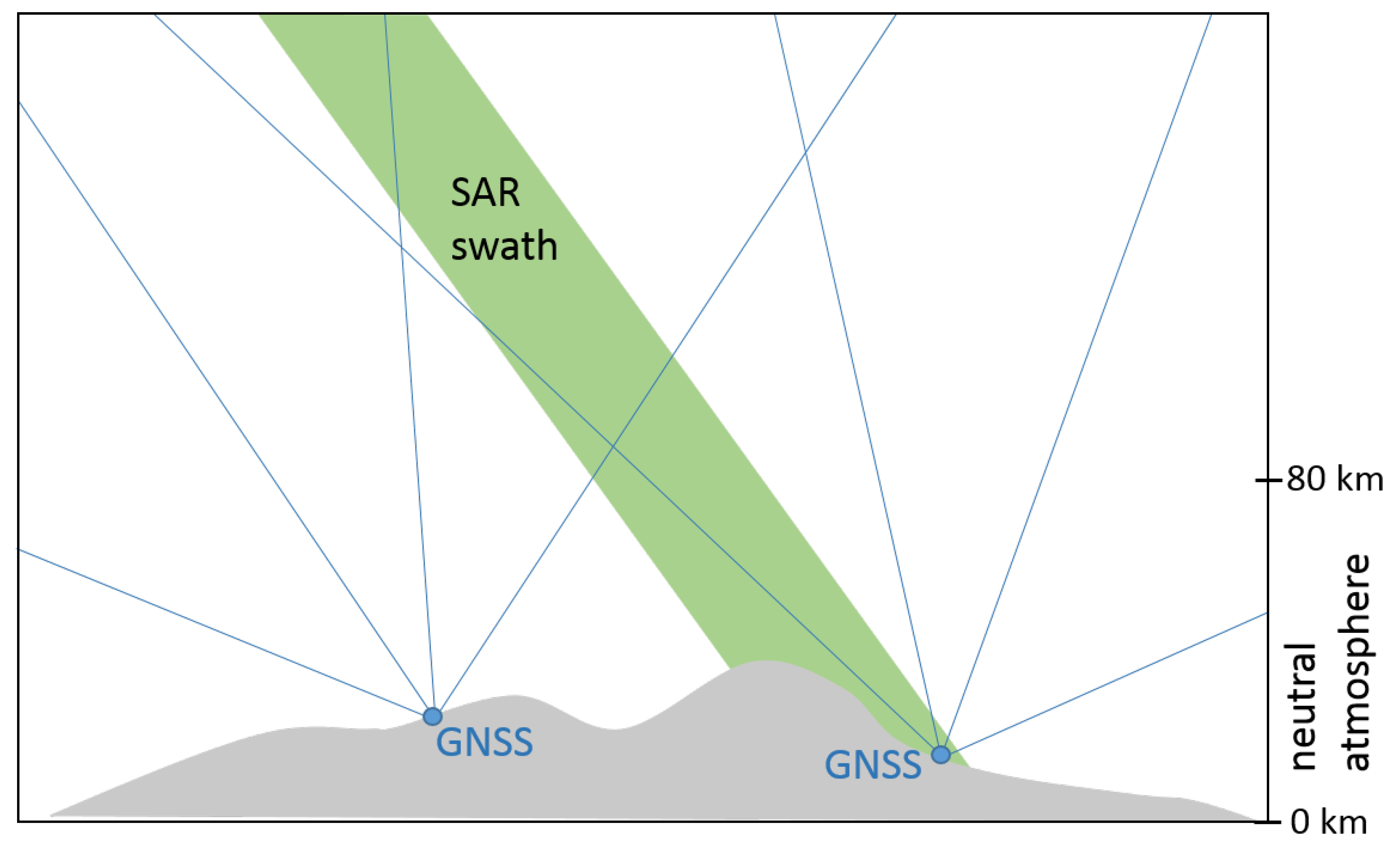
Figure 1 shows the geometry of the propagated signal in the neutral atmosphere. The SAR satellites’ orbits are located at around 800 km, while for GNSS it is around 20,000 km (depending on the system). The chosen X-band SAR signal propagates only along a very narrow range of incidence angles (here between
and
), whereas, the GNSS estimates are derived from a large set of views to the satellites spread over a wide range of different directions (here the zenith angles take values from
to
).
The test site selected for this work is a mountainous area of approximately 15 km × 25 km located in the canton of Valais, over Matter Valley, Swiss Alps. The altitudes of the area vary from around 1100 m to 4100 m above mean sea level (amsl). This region is chosen for two reasons: (a) the high mountains are a special case as the high relief is causing large spatial and temporal variability of the atmospheric signals and (b) this particular region has active landslides, rock slides and rockfalls [
7].
2.1. Synthetic Aperture Radar (SAR)
The interferometric data stack used in this work consists of 32 COSMO-SkyMed stripmap SAR repeat-pass acquisitions in a snow-free time period from June to October between 2008–2013. All the acquisitions were taken at a similar time, around 17:45 UTC. COSMO-SkyMed is an X-band satellite with the corresponding wavelength of
= 3.12 cm. For such frequencies, ionospheric effects are often ignored [
36], thus, we assume that the atmospheric phase component comes from the neutral atmosphere only. The footprint of the satellite image is depicted in
Figure 2 on top of the topography of the area (yellow parallelogram).
2.2. Global Navigation Satellite Systems
We focus on exploring the existing network of GNSS stations instead of setting up new stations.
Figure 2 shows the permanent GNSS stations in the vicinity of the selected area. We test both the geodetic permanent stations (red dots) and low-cost L1-only GPS permanent stations (green stars).
2.2.1. Geodetic Stations
The GNSS zenith tropospheric delays (
) and horizontal gradients are estimated with 1 h resolution by the Swiss Federal Office of Topography (swisstopo (
www.swisstopo.admin.ch)). Two networks are used: the Automated GNSS Network for Switzerland (AGNES) and permanent GNSS network of ETH Zürich installed in the alpine region of Valais within the framework of the project Coupled Seismogenic Geohazards in Alpine Regions (COGEAR (
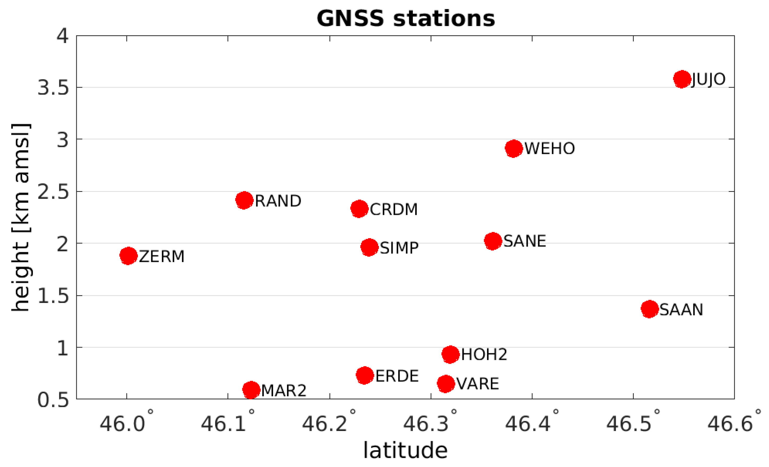
www.mpg.igp.ethz.ch/research/geomonitoring/cogear-gnss-monitoring.html)). In total, for the chosen period, up to 72 geodetic stations are used. Depending on the date, from five to 12 geodetic stations are operated close to the study area. The stations in the area are located at heights from 592 m to 3584 m asml. The heights are presented in
Figure 3. The
s are calculated in a double-difference post-processing mode from GPS and GLONASS observations using a development version 5.3 of Bernese software [
37]. The cut-off elevation angle is set up to
and the mapping function is VMF (Vienna Mapping Function) [
38].
2.2.2. Low-Cost L1-Only X-Sense Stations
A network of low-cost L1-only GPS stations was installed within a region of the study as a part of X-Sense project of nano-tera.ch (
www.nano-tera.ch/projects/227.php), a program of Swiss National Science Foundation [
39]. There are 32 stations located in an area of approximately 7 km × 7 km in the Randa Valley.
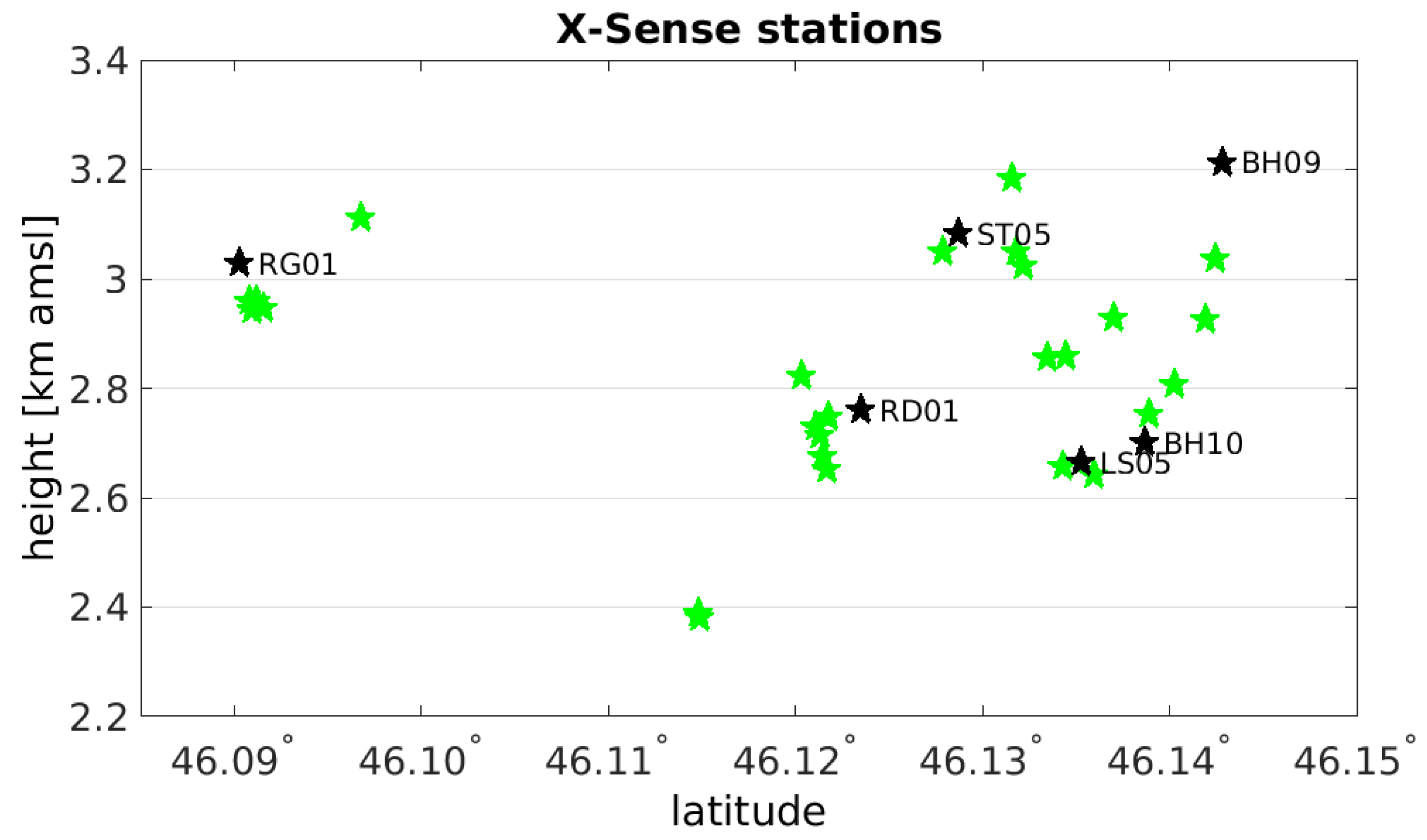
Figure 2 shows the locations of the stations (marked in green) and
Figure 4 depicts the height distribution of the X-Sense stations. The stations are located at altitudes of 2380–3213 m asml. The stations are equipped with single frequency (L1) receivers, thus, the
s are calculated in a relative sense referenced to the COGEAR station RAND, which is also located within the study area. The station RAND has been operated only since July 2012; thus, the X-Sense stations can only support the interpolation models for 11 acquisitions that took place in years 2012–2013. The
s are estimated without horizontal gradients with 1 h resolution using Bernese version 5.2 software [
37]. The Niell mapping function [
40] is used and the cut-off elevation angle is set to
, due to the possible obstructions of visibility.
3. Methodology
To compare the tropospheric delays estimates from two different space-borne techniques, namely GNSS and InSAR, we must reduce them to the same form and location. From InSAR, we calculate the phase differences, which are converted to the difference slant tropospheric delays (). From GNSS, we calculate the s at permanent stations. Then, we interpolate the GNSS s to the locations of persistent scatterers and convert them to s. In this section, we describe the methodology of these conversions in more detail.
3.1. Persistent Scatterer Interferometry
PSI [
5,
6,
41,
42] is a state-of-the-art method for deformation assessments with space-borne SAR data. PSI attempts to identify long-term temporally coherent targets for which the deformation phase can be separated from other sources of interferometric phase such as the atmosphere-induced phases and phase contributions induced by initially unknown residual topographic height differences with respect to a reference digital elevation model. In our work, we use an interferometric stack that was processed using the Interferometric Point Target Analysis (IPTA) module of the GAMMA software [
8,
43,
44].
An initial list of PS candidates is set up based on high temporal stability of the backscattering and low spectral diversity. The interferometric phases across the stack are double-differenced relative to a reference (master) acquisition and a reference point in the scene. The reference acquisition is on 20 September 2010, 17:46:45, which is roughly in the middle of all acquisition times. The reference point is shown in
Figure 5a and
Figure 6 as a white star.
The atmospheric phases separated from deformation and residual topography are isolated with a spatio-temporal filtering of the phase values. We assume that the atmospheric phases are spatially correlated to a certain extent while being uncorrelated from one pass to the next (given several weeks of separation among the repeat passes). The atmospheric phases estimated for the PS are low-pass filtered and spatially interpolated over the scene for example with a kriging interpolator [
5,
8]. The PS candidate list is iteratively refined using least-squares regression with quality control at each iteration [
41]. After several iterations, 326,552 PS have been identified within the chosen area. The unwrapped atmospheric phases,
(relative to the reference acquisition and reference point), estimated after the final refinement step are used to compute the
as follows:
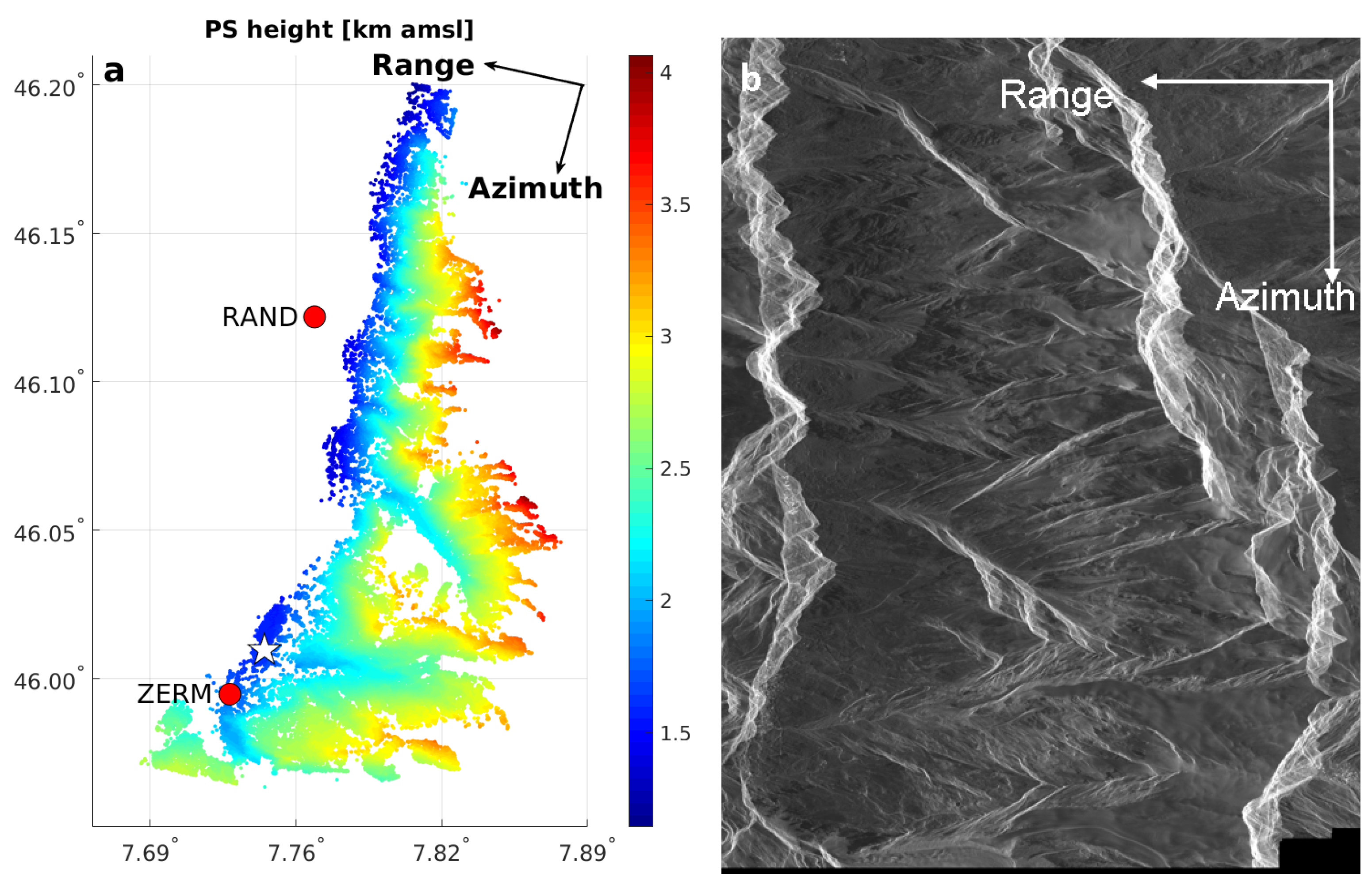
Figure 5a shows the heights of the identified PS points. The heights are spread between 1.1 km and 4 km amsl. The average intensity of the SAR image in the radar coordinates (range and azimuth) is shown in
Figure 5b. In the geographical coordinates, the descending COSMO-SkyMed satellite passes approximately from the north to the south and the radar looks to the west. Thus, the west side of the valley is affected by layover in the SAR images and the PS points are mostly located on the east side. By definition, a persistent scatterer is one single dominant scatterer per resolution cell. Thus, a layover induced by the mountain ridge leads to a very small number of PS being detected in the areas affected by layover.
3.2. Calculation of GNSS-Based Interpolation Models
The GNSS measurements are conducted for relatively few stations compared to the number of identified PS points. However, by taking advantage of a diversified height distribution of the stations, we can calculate the GNSS-based tropospheric estimates for all the PS. The chosen interpolation method is the least-squares collocation technique using an in-house developed software COMEDIE [
30,
31]. In the collocation technique, each measurement is divided into the deterministic part, the correlated stochastic part (signal) and the uncorrelated stochastic part (noise). With the estimated coefficients of the deterministic part and the signal, the considered parameters such as
can be interpolated at any given position and time. The deterministic model of
is given as:
where
x,
y,
z,
t are the Swiss projected coordinates LV03, orthometric height and time of the investigated point;
,
,
,
are the coordinates, height and time of the reference point (average point from all the observations in one time batch),
is the
at the reference position and time,
is the scale height (the increase in altitude for which the value of
decreases by a factor of
e) and
are the gradient parameters in
, and time, respectively.
The correlated stochastic part is assumed to be normally distributed with mean 0 and the covariance matrix
, which is chosen to be:
where
is the a-priori variance of the signal,
,
,
,
are the projected Swiss coordinates, orthometric height, and time of observation
i,
,
,
,
are the coordinates, height and time of observation
j,
= 4 km is a parameter modifying the correlation lengths as a function of height,
= 50 km,
= 50 km,
= 1 km,
= 1.7 h are the empirically determined correlation lengths of space and time. These collocation models have already been tested for the interpolation of GNSS data in [
34,
35]. In [
35], the cross-validation was performed for the stations in the similar area as in this study. The average bias between the reference stations and the interpolation models was close to 0 mm with 4 mm of standard deviation.
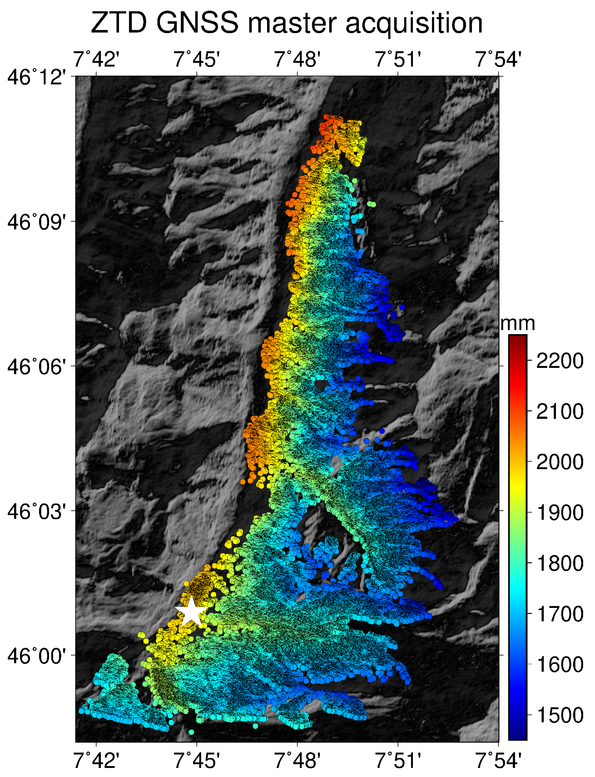
Figure 6 shows the absolute
s calculated from GNSS data for all 326,552 PS for the master acquisition. To calculate the slant tropospheric delays (
), we map the
s with a simple mapping function:
where
is the incidence (zenith) angle of the COSMO-SkyMed satellite. For this simple mapping function approach, it is recommended to use the exact incidence angle for each pixel of an InSAR image [
15], not an averaged one nor the one in the middle of the scene. For our study area, the angles vary from
in the near-range to
in the far-range.
From the absolute
s, we calculate the
for each point
and time
t as:
where
is the time of the master acquisition and
is the radar reference point on ground.
4. Results and Discussion
We compute the GNSS and InSAR-based relative tropospheric delay estimates for all the 32 acquisitions. Due to the relative nature of the delays, we cannot compare them for the master acquisition. Moreover, we removed three of the acquisitions from the comparisons due to unwrapping errors in PSI processing. For the 28 remaining dates, we assess the agreement between the two techniques using 4 metrics with the following assumptions of the level of the agreement:
R [unitless]: Pearson’s correlation coefficient, which measures the values of linear correlation between two variables; it takes values from −1 to 1, with 1 being a full correlation,
means strong correlation,
means moderate,
weak and
a very weak or no correlation [
45].
Index of Agreement (
) [unitless]: developed by [
46] is a standard measure of a model prediction error; it takes values between 0 and 1; where 1 is a perfect match,
means good agreement,
moderate,
poor and
very poor agreement. The
can detect additive and proportional differences between the two models; however, it is very sensitive to extreme values [
47].
bias [mm]: the difference between and averaged over the study area; it describes the model tendency of an overestimation (bias > 0) or underestimation (bias < 0); mm means good agreement, 2 mm mm moderate, 4 mm mm poor and mm very poor agreement.
standard deviation () [mm] of the differences is a measure of a variation of data; mm means good agreement, 3.5 mm mm moderate, 5 mm mm poor and mm very poor agreement.
The levels of agreement for biases and s are decided arbitrarily based on the experience of the authors to make the interpretation of the results easier.
4.1. Comparisons of InSAR and GNSS Tropospheric Estimates
Firstly, we compare the InSAR delays with the GNSS-based estimates computed from the geodetic network of Switzerland (AGNES and COGEAR).
Table 1 presents an overview of the statistics for all 28 acquisitions, sorted by the level of the agreement.
Table 1 presents on average 7 acquisitions with a good agreement, 8 with moderate, 8 with poor, and 5 with very poor agreement. In
Section 4.3 we discuss the possible reasons for the good/poor agreement for particular acquisitions. However, firstly, we take a closer look at some examples of both situations.
Figure 7 shows an example of a good agreement between the two techniques for one day 23 September 2011.
Most of the dates of good agreement between GNSS and InSAR look similar to
Figure 7. For such days, the variability of GNSS estimates is high, almost as high as for InSAR. However, InSAR measurements have much higher spatial resolution and sometimes the estimates from InSAR are more detailed than for GNSS. This behavior is visible in the correlation plots as ‘tails’ that are the variability of the delay captured by InSAR but not by GNSS.
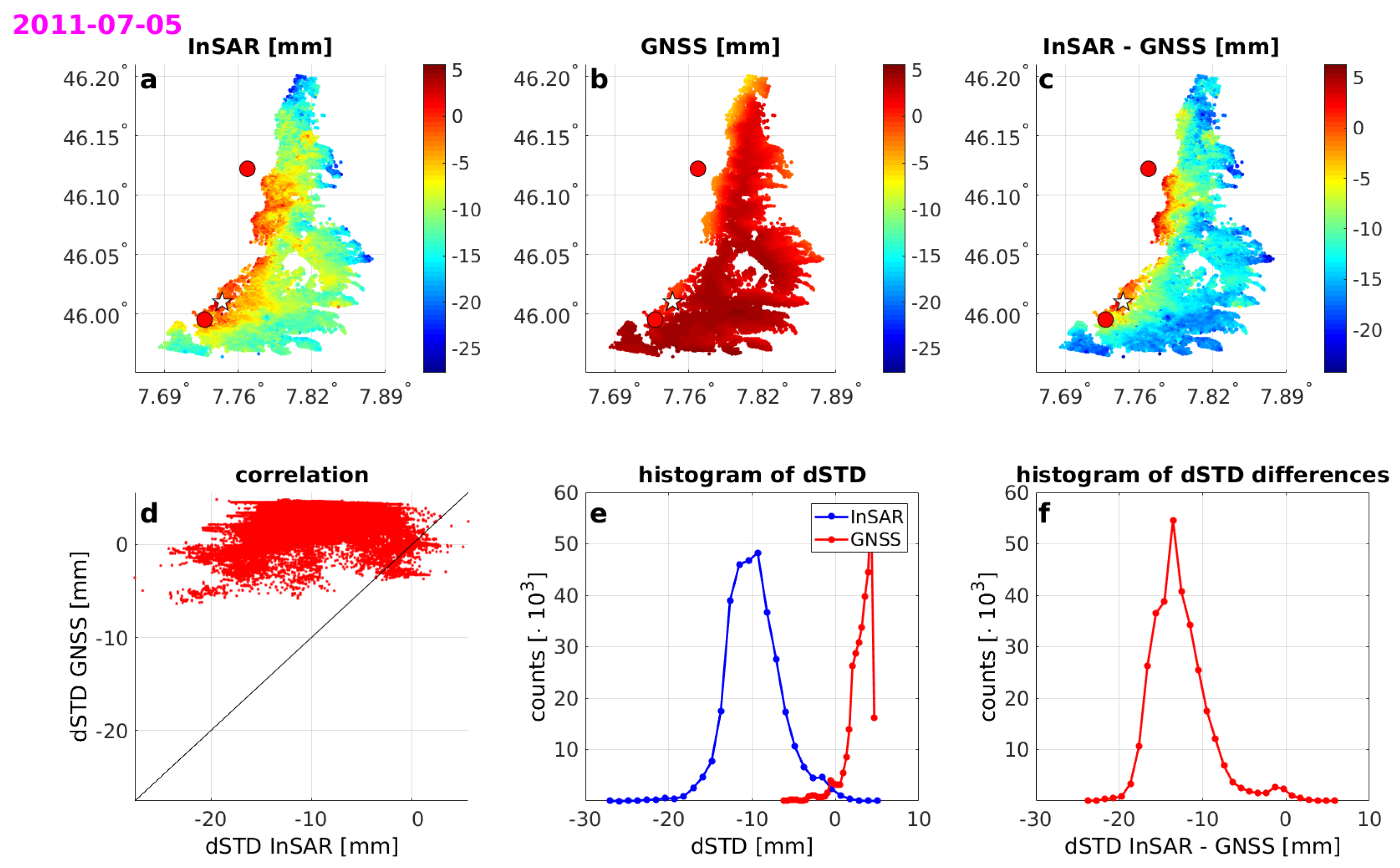
Figure 8 depicts the worst agreement between InSAR and GNSS from all dates (5 July 2011). The correlation coefficient for this date is equal to only 0.07. As shown in
Figure 8b, the estimates based on GNSS are almost constant. This is the most common feature for the days with poor agreement—the GNSS estimates are very stable, almost constant, while the InSAR estimates show variability. An interesting example of poor agreement is day 4 September 2010, presented in
Figure 9. Visually, the agreement could be evaluated as good, especially looking only at the histograms, but in the northern part of the area, there is a negative correlation between InSAR and GNSS. This could be only explained by some very local tropospheric conditions that cannot be captured by the sparse GNSS data.
Considering the spatial location of the PS points, the highest agreement is close to the only GNSS station within the area, ZERM. The agreement between the techniques for the PS points located around this station is usually good, even for acquisitions that are overall classified as poor. There is another GNSS station, RAND, which is located close to the PS points, but on the other side of the valley and no PS were found at the exact location of the station due to layover. Nonetheless, this station influences the GNSS-based estimates. RAND is located at around 2.5 km amsl and the closest (in a planar sense) PS points are in the valley at around 1.5–2 km amsl. Thus, the GNSS estimates for these points, influenced by RAND, are often underestimated, which manifests as positive differences between InSAR and GNSS for that area. This behavior is also visible for other dates, which are not shown here.
In general, the GNSS estimates are highly dependent on the topography. The PS heights, as shown in
Figure 5, reach up to 4 km amsl, while the two stations located in the closest vicinity, RAND and ZERM are located at 2.5 and 2 km amsl respectively. Thus, there is a possibility of overestimating the delays at higher altitudes (located in the northeast side of the area). On the other hand, in that area, the slope is very steep, and the height differences are very rapid. This is also a challenge for the InSAR technique—estimating the points that are very close horizontally but with large height differences. Although it is evidently a challenging area to estimate, there is no clear pattern of the InSAR-GNSS differences. In
Figure 7, the GNSS is underestimated compared to InSAR, in
Figure 8 overestimated and in
Figure 10 there is no relation between the PS heights and the agreement. There is one batch of PS points where the two techniques differ significantly for many of the acquisitions. It is in the south-west of the area at altitudes 2.5–3 km amsl, which is much higher than the altitudes of the other PS points that are horizontally close. There are usually large differences between the techniques for this area, even for days of overall good agreement. The probable reason is that the closest points in a planar way are actually located at much higher altitudes and the InSAR estimates may be wrong due to erroneous phase wrapping. Such situations occur sometimes for PSI processing in the high mountains and we see a potential in using GNSS-based estimates for detecting them.
4.2. Comparisons of InSAR and GNSS/X-Sense Tropospheric Estimates
Furthermore, we test if adding the low-cost L1-only stations can improve the agreement between the techniques.
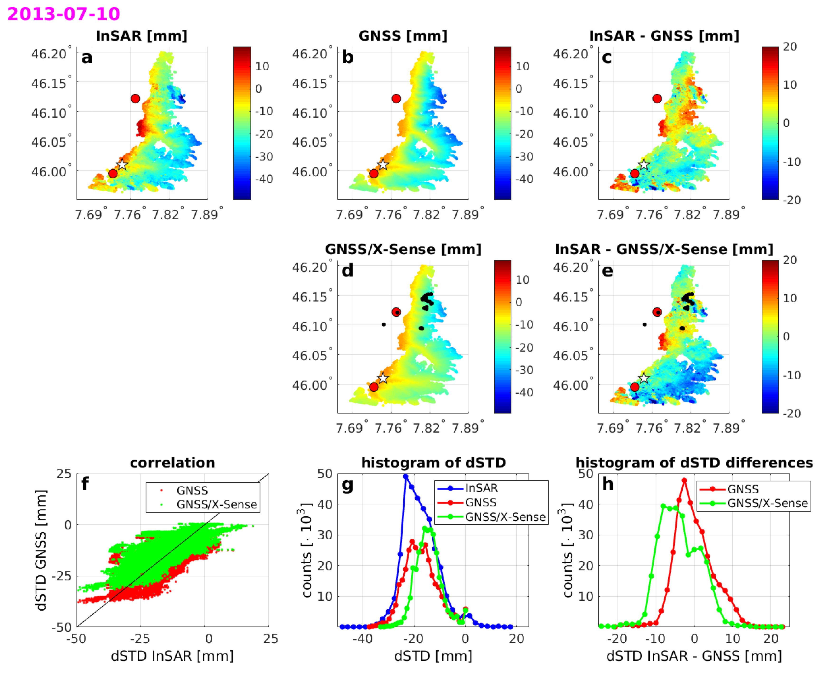
Figure 10 shows an example of the tropospheric delay estimates based on three data sources: ‘InSAR’, ‘GNSS only’ and ‘GNSS/X-Sense’ for one date 10 July 2013.
The
estimates based on the ‘GNSS/X-Sense’ data set show even less variability than ‘GNSS only’. A possible reason may be that we take too many stations over too small area that are located at altitudes within less than 1 km. Thus, the vertical distribution of the stations may not be sufficient. To test this hypothesis, we take only six X-Sense stations out of 32 into the collocation procedure. The selected stations are nearly uniformly distributed as shown in
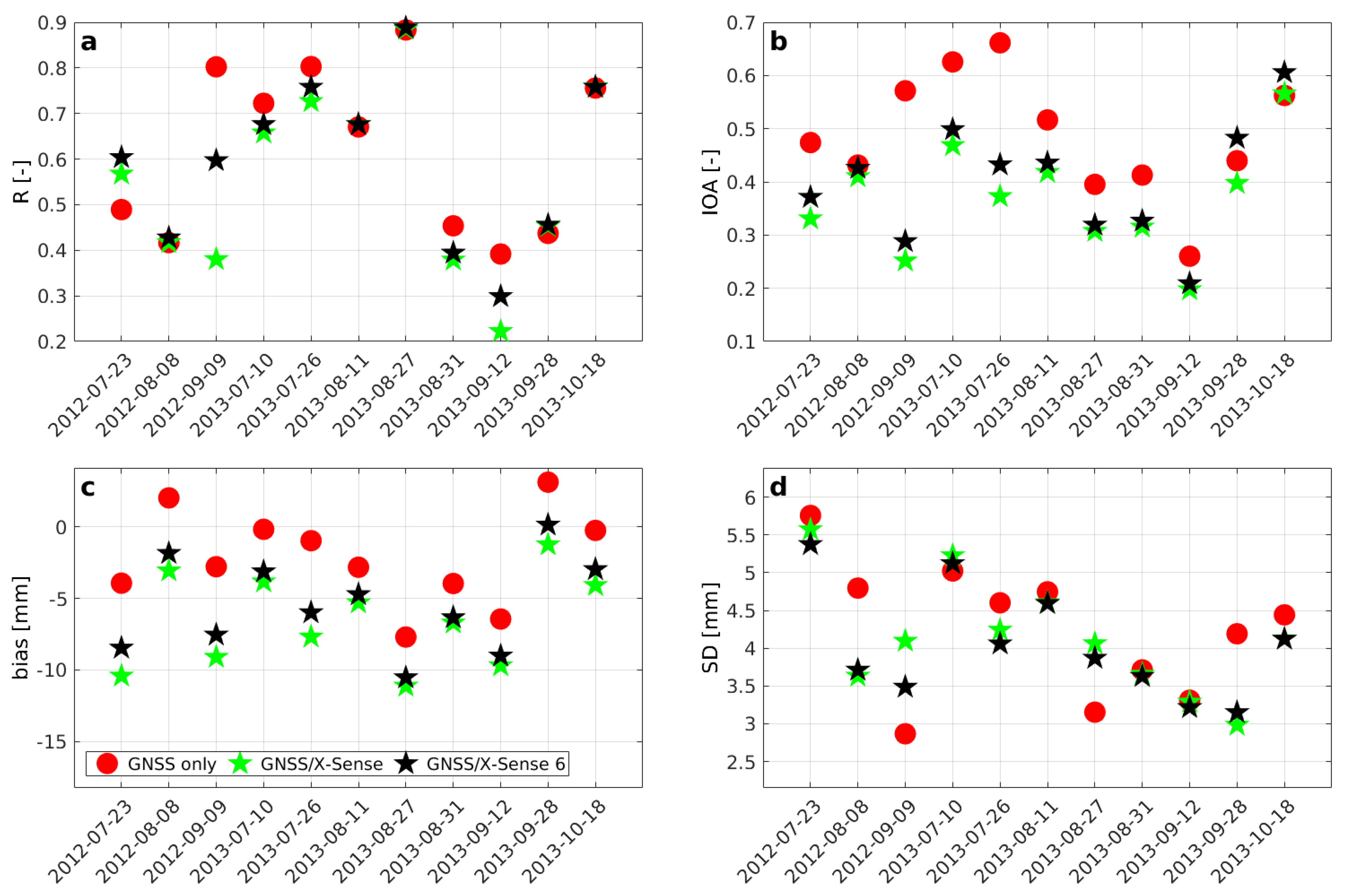
Figure 4. Using the ‘GNSS/X-Sense 6’ data set, we achieve a slight improvement compared to ‘GNSS/X-Sense’, although, for most of the days, it is still worse than ‘GNSS only’ set. Correlation coefficients,
s, biases and
s for all three data sets are shown in
Figure 11. The X-Sense data are only available from July 2012; thus, the statistics are only calculated for the corresponding 11 acquisitions of COSMO-SkyMed.
Unfortunately, adding the X-Sense data does not improve the agreement between InSAR and GNSS for the area of this study. Thus, we test if it can improve the estimates only for the area covering the X-Sense stations.
Figure 12 shows the estimates analogical to depicted in
Figure 10, for the same date 10 July 2013, but for the limited area and
Figure 13 shows the statistics calculated only for the limited area.
For the limited area, the estimates from ‘GNSS/X-Sense’ data set are in a higher agreement with InSAR than for the whole area, but on average the agreement is still worse than for the ‘GNSS only’ data set. However, for some dates, the s for the combined estimates are higher and the biases are smaller. A positive impact of using X-Sense stations is that the s of the differences between techniques for almost all dates are smaller for ‘GNSS/X-Sense’ than ‘GNSS only’.
The ‘GNSS/X-Sense 6’ data set is almost always slightly better or similar to ‘GNSS/X-Sense’ set, which includes all of the X-Sense stations. The low-cost, L-1 only X-Sense stations have of course worse quality than GNSS geodetic stations. The comparisons show that unfortunately, taking such low-cost stations into combinations with geodetic stations can deteriorate the results, especially in the areas where there are no stations and we have to extrapolate (as shown in
Figure 10 and
Figure 11). For the limited area that included the X-Sense stations, the combination model is still worse than ‘GNSS only’, which can be attributed to the quality of the X-Sense stations.
It is worth further noting that the agreement of the ‘GNSS only’ subset with the InSAR estimates is worse for the limited area than it is for the entire area. The closest GNSS station, RAND is located on the other side of the valley where there are no PS points, due to a layover. This station is located also at higher altitude than the closest PS points in the valley. This affects the GNSS-based model and can explain why the general agreement between GNSS and InSAR deteriorates in the limited area. However, for the acquisition depicted in
Figure 12, the differences are not height dependent. There are some very local changes in
captured by InSAR but not by either ‘GNSS only’ nor ‘GNSS/X-Sense’ estimates. For this scene, the agreement between the techniques is the worst for the area of X-Sense stations. Thus, the agreement of GNSS is worse for the limited area compared to the entire area. Moreover, there are a few acquisitions where the correlation for the limited area is actually negative, which deteriorates the agreement for the entire scene.
4.3. Discussion
The agreement between the InSAR and GNSS-based tropospheric delays differs spatially within one acquisition and temporally between different acquisitions. The reasons of the spatial differences are discussed in
Section 4.1 and
Section 4.2. Here, we investigate the reasons of the differences between the techniques for different acquisitions. Firstly, we test if the agreement is correlated with meteorological conditions. We compare the GNSS estimates with NWM ERA-Interim provided by European Centre for Medium-Range Weather Forecasts (ECMWF (
https://www.ecmwf.int/)). This model is calculated with a very sparse resolution of approximately 80 km. To compare the weather situation with the delays, we interpolate the meteorological parameters of ERA-Interim to the locations of chosen uniformly distributed PS points (approx. 5000 points) using the GOP-TropDB–TropModel online service (
http://www.pecny.cz/GOP-TropDB/form-online/) [
48,
49]. We compare the values of the water vapor partial pressure (
), temperature, and air pressure with the agreements between InSAR and GNSS. For temperature and air pressure there is no visible relation between the parameters and the agreement. However, there is a weak correlation between
and the agreement.
Figure 14 shows the average values and
s of water vapor averaged over the entire area. The colors for each day indicate the agreement for that day consistent with
Table 1.
For many days with poor agreement, the s of values are lower than for days with good agreement. This may indicate that a better agreement can be achieved for days with more variability of the troposphere which is mostly influenced by the variability of . Better agreement is also achieved for days for which s are closer to the s of the master acquisition. For the average values, there is no such correspondence.
We test further the influence of the tropospheric conditions on the agreement between InSAR and GNSS. The standard deviation of
GNSS is the simplest measure of the tropospheric variability in space. Last column of
Table 1 presents these
s. There is a visible relation between the agreement and the GNSS
, i.e., for the days with a good agreement the GNSS
is relatively high (>5 mm) compared to the days with poor agreement where the
is relatively low (<3 mm). This may indicate that for our case study, the good agreement between GNSS and InSAR is obtained for the days of more spatially varying troposphere. The reason for that may be that master acquisition has been chosen to be of calm tropospheric conditions. The
s are relative to the master acquisition and thus, for days of calm troposphere, when the GNSS
s are too similar to the master acquisition, the GNSS
s are too constant.
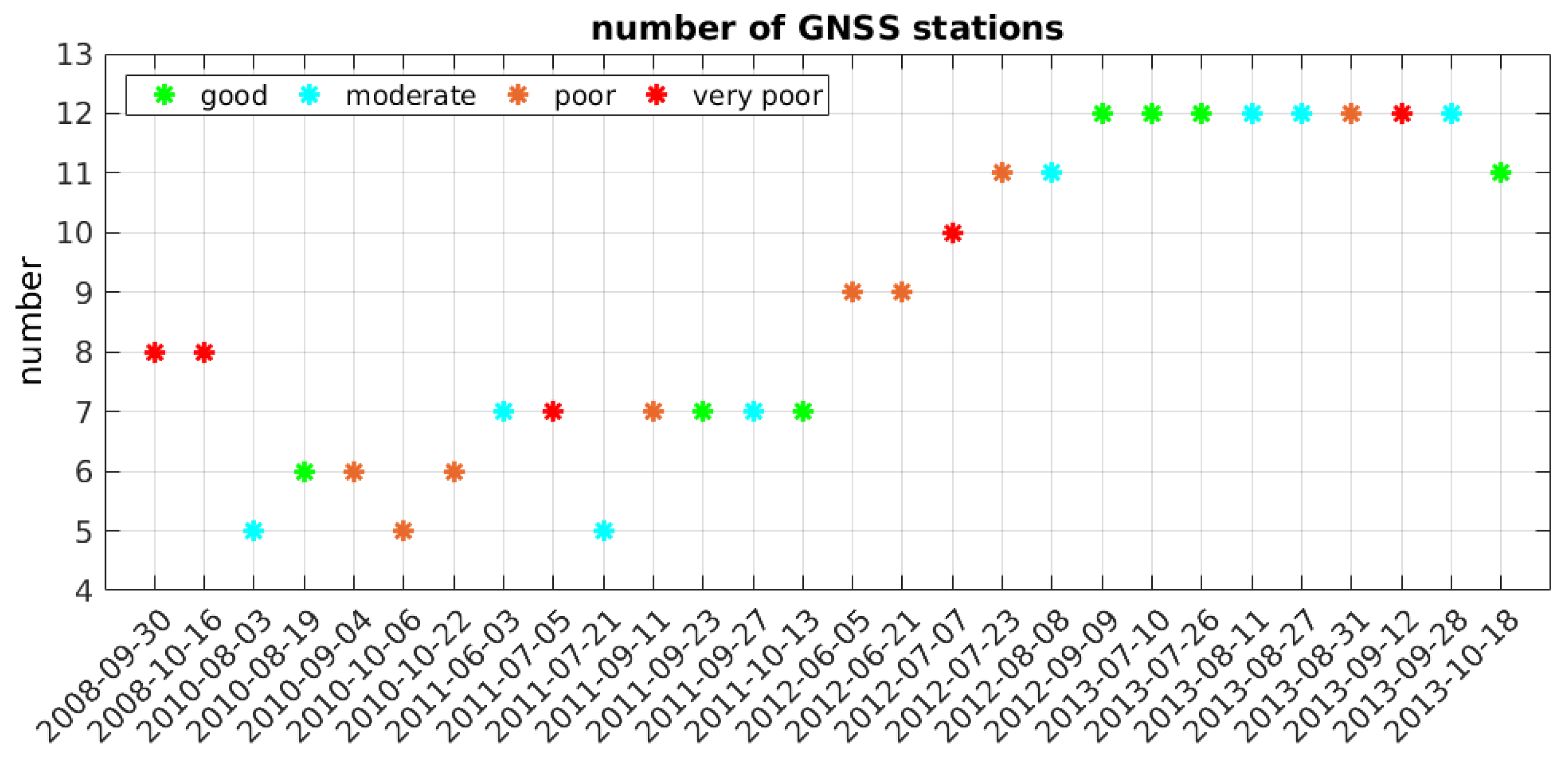
Another characteristic that can differentiate between the particular days is the number of GNSS stations in the closest vicinity of the study area. There are less stations for the earlier dates (from five to eight) and more stations (from 9 to 12) starting from 2012, when the majority of the COGEAR stations was installed.
Figure 15 shows the number of stations for each day, where the colors indicate the level of agreement.
As shown in
Figure 15, for the earlier dates, there are more times with poor agreement than for the later, but it is difficult to see a clear relation between the number of stations and the level of the agreement. For example, there are three days with only 5 stations available, and for two of them the agreement is moderate, while only for one it is poor. Also, for the days with the maximum number of stations, there are 5 days with good or moderate agreement, but two days with poor. On the other hand, the average metrics calculated from years 2012–2013, where there are more stations are similar or better than for all the dates. For
R and
there is almost no difference, but
from the two-year period equals to 0.49 (compared to 0.42 from all acquisitions) and the largest improvement is with bias, which equals to −2.1 mm averaged from two last years and −5.5 mm for all the acquisitions.
5. Conclusions
We compared the estimates obtained from two geodetic space-borne techniques, InSAR and GNSS, for 32 SAR acquisitions spanned over a period of five years. Three of the acquisitions were removed from the analysis due to phase unwrapping errors in the interferometric processing. We divided the remaining 28 pairs into days with good, moderate, poor and very poor agreements based on the correlation coefficients, , biases, and s between the data sets. The good or moderate agreement was achieved for more than a half of the acquisitions. We also incorporated the information from low-cost GPS-only stations located in Randa Valley for 11 acquisitions where the data were available. Unfortunately, this inclusion did not improve the overall agreement between the two techniques. The only improved measure was the of the differences for a limited area, where the X-Sense stations are located.
The differences in the agreement between the two techniques varied spatially within one interferogram but also temporally between different acquisitions. Spatially, the best agreement was obtained for PS points located close to GNSS station ZERM. There is another GNSS station (RAND), close to the study area, but on the other side of the Randa Valley. The GNSS estimates from RAND had rather negative impact on the agreement, because the station is located much higher than horizontally close PS points. Similar impact can be seen for some of the PS points that are located at much higher altitudes than the points nearby. For these points, the agreement between the techniques was always the worst.
Temporally, the agreement for different acquisitions also varied. We investigated the possible reasons of the poor agreement between techniques, considering the meteorological conditions in the area, the tropospheric conditions and the number of available stations. There is a weak correlation between the agreement and the variability of water vapor—for days of higher variability, the agreement is better. The variability of water vapor is directly linked to the variability of troposphere, which can be expressed for example in standard deviations of the GNSS s. For days with higher s of the GNSS estimates, the agreement between techniques was higher. The agreement was also moderately dependent on the number of stations. For the years 2012–2013, where there are mores stations available in the vicinity of the area, there were more instants of a good agreement and some statistics, namely biases and s were improved.
As expected, there occurred considerable differences between the GNSS and the InSAR estimates in the challenging alpine conditions, due to different spatio-temporal characteristics of both techniques. The geometry of the satellites is different. The SAR signal propagates only in a narrow swath from one direction, while the GNSS estimates are obtained from a wide range of angles. This is one of the limiting factors, why the two approaches lead to sometimes significantly different delays. Moreover, it may be impossible to capture the spatial variability of the troposphere with only a few GNSS stations in as much detail as with PSI at X-band, which has a much higher sensitivity to the tropospheric delay than the L-band GNSS on top of the much higher spatial resolution. On the other hand, the InSAR estimates will never reach the temporal resolution of GNSS stations, although, the planned new geosynchronous SAR missions are designed to provide a higher temporal resolution. Nonetheless, this study showed that it is possible in some cases to obtain a good level of agreement between techniques, which may open the possibility of combining these techniques into one tropospheric product.
Author Contributions
Conceptualization, K.W., M.A.S., A.G., T.S. and O.F.; methodology, K.W., M.A.S. and T.S.; validation, K.W., M.A.S.; formal analysis, K.W.; investigation, K.W., M.A.S.; resources, T.S.; data curation, T.S.; writing—original draft preparation, K.W. and M.A.S.; writing—review and editing, A.G., T.S., O.F.; visualization, K.W., M.A.S.; supervision, A.G., O.F.; project administration, A.G., O.F.; funding acquisition, A.G., O.F.
Funding
This research has been partially funded by the Swiss Federal Office of Environment project ‘Geodetic geomonitoring: Tropospheric corrections for satellite InSAR by Model and GNSS’ (14.0022.PJ). The research has also been partially funded by the Swiss Space Office, State Secretariat for Education and Research of the Swiss Confederation (SER/SSO), in the frame of the MdP2012 ‘Space Technology Studies’ and internal ETH funding.
Acknowledgments
We thank Elmar Brockmann from swisstopo for providing AGNES/COGEAR GNSS data, Philippe Limpach from BSF Swissphoto for carrying out path delays calculations from X-Sense data and Jan Dousa from Geodetic Observatory Pecny for providing the ERA-Interin interpolations. The interferometric data stack used in this work is a COSMO-SkyMed Product-©ASI—Agenzia Spaziale Italiana (2013). M.A. Siddique’s research work was performed while he was with ETH Zurich, funded by the Swiss Space Office, State Secretariat for Education and Research of the Swiss Confederation (SER/SSO), in the frame of the MdP2012 ‘Space Technology Studies’ and by internal ETH funding.
Conflicts of Interest
The authors declare no conflict of interest.
Abbreviations
The following abbreviations are used in this manuscript:
| AGNES | Automated GNSS Network for Switzerland |
| COGEAR | Coupled Seismogenic Geohazards in Alpine Regions |
| COMEDIE | Collocation of Meteorological Data for Interpretation and Estimation of Tropospheric Path delays |
| DEM | Digital Elevation Model |
| dSTD | difference Slant Tropospheric Delay |
| ECMWF | European Centre for Medium-Range Weather Forecasts |
| GPS | Global Positioning System |
| GNSS | Global Navigation Satellite System |
| InSAR | SAR Interferometry |
| IOA | Index of Agreement |
| NWM | Numerical Weather Model |
| PS | Persistent Scatterer |
| PSI | Persistent Scatterer Interferometry |
| SAR | Synthetic Aperture Radar |
| SD | Standard Deviation |
| STD | Slant Tropospheric Delay |
| WV | Water Vapor |
| ZTD | Zenith Tropospheric Delay |
References
- Strozzi, T.; Ambrosi, C.; Raetzo, H. Interpretation of aerial photographs and satellite SAR interferometry for the inventory of landslides. Remote Sens. 2013, 5, 2554–2570. [Google Scholar] [CrossRef]
- Tofani, V.; Raspini, F.; Catani, F.; Casagli, N. Persistent Scatterer Interferometry (PSI) technique for landslide characterization and monitoring. Remote Sens. 2013, 5, 1045–1065. [Google Scholar] [CrossRef]
- Lambiel, C.; Delaloye, R.; Strozzi, T.; Lugon, R.; Raetzo, H. ERS InSAR for assessing rock glacier activity. In Proceedings of the Ninth International Conference on Permafrost, Fairbanks, AK, USA, 29 June–3 July 2008; Kane, D.L., Hinkel, K.M., Eds.; University of Alaska Fairbanks: Fairbanks, AK, USA, 2008; pp. 1019–1024. [Google Scholar]
- Kääb, A.; Huggel, C.; Fischer, L.; Guex, S.; Paul, F.; Roer, I.; Salzmann, N.; Schlaefli, S.; Schmutz, K.; Schneider, D.; et al. Remote sensing of glacier-and permafrost-related hazards in high mountains: An overview. Nat. Hazards Earth Syst. Sci. 2005, 5, 527–554. [Google Scholar] [CrossRef]
- Ferretti, A.; Prati, C.; Rocca, F. Permanent scatterers in SAR interferometry. IEEE Trans. Geosci. Remote Sens. 2001, 39, 8–20. [Google Scholar] [CrossRef]
- Kampes, B.M.; Adam, N. The STUN algorithm for persistent scatterer interferometry. In Proceedings of the European Space Agency Fringe 2005 Workshop, Frascati, Italy, 28 November–2 December 2005; ESA Publications Div.: Neuilly-sur-Seine, Noordwijk, 2006; Volume 610. [Google Scholar]
- Strozzi, T.; Raetzo, H.; Wegmüller, U.; Papke, J.; Caduff, R.; Werner, C.; Wiesmann, A. Satellite and terrestrial radar interferometry for the measurement of slope deformation. In Engineering Geology for Society and Territory—Volume 5; Springer: Berlin, Germany, 2015; pp. 161–165. [Google Scholar]
- Siddique, M.A.; Strozzi, T.; Hajnsek, I.; Frey, O. A Case Study on the Correction of Atmospheric Phases for SAR Tomography in Mountainous Regions. IEEE Trans. Geosci. Remote Sens. 2018, 57, 416–431. [Google Scholar] [CrossRef]
- Zebker, H.A.; Rosen, P.A.; Hensley, S. Atmospheric effects in interferometric synthetic aperture radar surface deformation and topographic maps. J. Geophys. Res. Solid Earth 1997, 102, 7547–7563. [Google Scholar] [CrossRef]
- Hanssen, R.F.; Weckwerth, T.M.; Zebker, H.A.; Klees, R. High-resolution water vapor mapping from interferometric radar measurements. Science 1999, 283, 1297–1299. [Google Scholar] [CrossRef]
- Hanssen, R.F. Radar Interferometry: Data Interpretation and Error Analysis; Springer Science & Business Media: Berlin, Germany, 2001; Volume 2. [Google Scholar]
- Elliott, J.; Biggs, J.; Parsons, B.; Wright, T. InSAR slip rate determination on the Altyn Tagh Fault, northern Tibet, in the presence of topographically correlated atmospheric delays. Geophys. Res. Lett. 2008, 35. [Google Scholar] [CrossRef]
- Doin, M.P.; Lasserre, C.; Peltzer, G.; Cavalié, O.; Doubre, C. Corrections of stratified tropospheric delays in SAR interferometry: Validation with global atmospheric models. J. Appl. Geophys. 2009, 69, 35–50. [Google Scholar] [CrossRef]
- Bekaert, D.; Hooper, A.; Wright, T. A spatially variable power law tropospheric correction technique for InSAR data. J. Geophys. Res. Solid Earth 2015, 120, 1345–1356. [Google Scholar] [CrossRef]
- Hobiger, T.; Kinoshita, Y.; Shimizu, S.; Ichikawa, R.; Furuya, M.; Kondo, T.; Koyama, Y. On the importance of accurately ray-traced troposphere corrections for Interferometric SAR data. J. Geod. 2010, 84, 537–546. [Google Scholar] [CrossRef]
- Nico, G.; Tome, R.; Catalao, J.; Miranda, P.M. On the use of the WRF model to mitigate tropospheric phase delay effects in SAR interferograms. IEEE Trans. Geosci. Remote Sens. 2011, 49, 4970–4976. [Google Scholar] [CrossRef]
- Mateus, P.; Nico, G.; Tomé, R.; Catalao, J.; Miranda, P.M. Experimental study on the atmospheric delay based on GPS, SAR interferometry, and numerical weather model data. IEEE Trans. Geosci. Remote Sens. 2013, 51, 6–11. [Google Scholar] [CrossRef]
- Kinoshita, Y.; Furuya, M.; Hobiger, T.; Ichikawa, R. Are numerical weather model outputs helpful to reduce tropospheric delay signals in InSAR data? J. Geod. 2013, 87, 267–277. [Google Scholar] [CrossRef]
- Foster, J.; Brooks, B.; Cherubini, T.; Shacat, C.; Businger, S.; Werner, C. Mitigating atmospheric noise for InSAR using a high resolution weather model. Geophys. Res. Lett. 2006, 33, L16304. [Google Scholar] [CrossRef]
- Williams, S.; Bock, Y.; Fang, P. Integrated satellite interferometry: Tropospheric noise, GPS estimates and implications for interferometric synthetic aperture radar products. J. Geophys. Res. Solid Earth 1998, 103, 27051–27067. [Google Scholar] [CrossRef]
- Van der Hoeven, A.; Hanssen, R.F.; Ambrosius, B. Tropospheric delay estimation and analysis using GPS and SAR interferometry. Phys. Chem. Earth 2002, 27, 385–390. [Google Scholar] [CrossRef]
- Fornaro, G.; D’Agostino, N.; Giuliani, R.; Noviello, C.; Reale, D.; Verde, S. Assimilation of GPS-derived atmospheric propagation delay in DInSAR data processing. IEEE J. Sel. Top. Appl. Earth Obs. Remote Sens. 2015, 8, 784–799. [Google Scholar] [CrossRef]
- Houlié, N.; Funning, G.J.; Bürgmann, R. Use of a GPS-derived troposphere model to improve InSAR deformation estimates in the San Gabriel Valley, California. IEEE Trans. Geosci. Remote Sens. 2016, 54, 5365–5374. [Google Scholar] [CrossRef]
- Del Soldato, M.; Farolfi, G.; Rosi, A.; Raspini, F.; Casagli, N. Subsidence evolution of the Firenze–Prato–Pistoia plain (Central Italy) combining PSI and GNSS data. Remote Sens. 2018, 10, 1146. [Google Scholar] [CrossRef]
- Yu, C.; Li, Z.; Penna, N.T. Interferometric synthetic aperture radar atmospheric correction using a GPS-based iterative tropospheric decomposition model. Remote Sens. Environ. 2018, 204, 109–121. [Google Scholar] [CrossRef]
- Strozzi, T.; Kääb, A.; Frauenfelder, R. Detecting and quantifying mountain permafrost creep from in situ inventory, space-borne radar interferometry and airborne digital photogrammetry. Int. J. Remote Sens. 2004, 25, 2919–2931. [Google Scholar] [CrossRef]
- Parker, A.L.; Featherstone, W.E.; Penna, N.T.; Filmer, M.S.; Garthwaite, M.C. Practical Considerations before Installing Ground-Based Geodetic Infrastructure for Integrated InSAR and cGNSS Monitoring of Vertical Land Motion. Sensors 2017, 17, 1753. [Google Scholar] [CrossRef]
- Alshawaf, F.; Hinz, S.; Mayer, M.; Meyer, F.J. Constructing accurate maps of atmospheric water vapor by combining interferometric synthetic aperture radar and GNSS observations. J. Geophys. Res. Atmos. 2015, 120, 1391–1403. [Google Scholar] [CrossRef]
- Bock, Y.; Wdowinski, S.; Ferretti, A.; Novali, F.; Fumagalli, A. Recent subsidence of the Venice Lagoon from continuous GPS and interferometric synthetic aperture radar. Geochem. Geophys. Geosyst. 2012, 13. [Google Scholar] [CrossRef]
- Eckert, V.; Cocard, M.; Geiger, A. COMEDIE:(Collocation of Meteorological Data for Interpretation and Estimation of Tropospheric Pathdelays) Teil I: Konzepte, Teil II: Resultate; Technical Report 194; Grauer Bericht; ETH Zürich: Zürich, Switzerland, 1992. [Google Scholar]
- Eckert, V.; Cocard, M.; Geiger, A. COMEDIE:(Collocation of Meteorological Data for Interpretation and Estimation of Tropospheric Pathdelays) Teil III: Software; Technical Report 195; Grauer Bericht; ETH Zürich: Zürich, Switzerland, 1992. [Google Scholar]
- Troller, M. GPS Based Determination of the Integrated and Spatially Distributed Water Vapor in the Troposphere; Geodätisch-geophysikalische Arbeiten in der Schweiz; Swiss Geodetic Commission: Zurich, Switzerland, 2004; Volume 67. [Google Scholar]
- Hurter, F.; Maier, O. Tropospheric profiles of wet refractivity and humidity from the combination of remote sensing data sets and measurements on the ground. Atmos. Meas. Tech. 2013, 6, 3083–3098. [Google Scholar] [CrossRef]
- Wilgan, K.; Hurter, F.; Geiger, A.; Rohm, W.; Bosy, J. Tropospheric refractivity and zenith path delays from least-squares collocation of meteorological and GNSS data. J. Geod. 2017, 91, 117–134. [Google Scholar] [CrossRef]
- Wilgan, K.; Geiger, A. High-resolution models of tropospheric delays and refractivity based on GNSS and numerical weather prediction data for alpine regions in Switzerland. J. Geod. 2019, 93, 819–835. [Google Scholar] [CrossRef]
- Meyer, F.J. Performance requirements for ionospheric correction of low-frequency SAR data. IEEE Trans. Geosci. Remote Sens. 2011, 49, 3694–3702. [Google Scholar] [CrossRef]
- Dach, R.; Lutz, S.; Walser, P.; Fridez, P. Bernese GNSS Software Version 5.2; Astronomical Institute, University of Bern: Bern, Switzerland, 2015. [Google Scholar]
- Boehm, J.; Werl, B.; Schuh, H. Troposphere mapping functions for GPS and very long baseline interferometry from European Centre for Medium-Range Weather Forecasts operational analysis data. J. Goephys. Res. Solid Earth 2006, 111. [Google Scholar] [CrossRef]
- Beutel, J.; Buchli, B.; Ferrari, F.; Keller, M.; Zimmerling, M. X-SENSE: Sensing in extreme environments. In Proceedings of the Design, Automation & Test in Europe Conference & Exhibition (DATE), Grenoble, France, 14–18 March 2011; pp. 1–6. [Google Scholar]
- Niell, A. Improved atmospheric mapping functions for VLBI and GPS. Earth Planets Space 2000, 52, 699–702. [Google Scholar] [CrossRef]
- Werner, C.; Wegmuller, U.; Wiesmann, A.; Strozzi, T. Interferometric point target analysis with JERS-1 L-band SAR data. In Proceedings of the IGARSS 2003, 2003 IEEE International Geoscience and Remote Sensing Symposium, Toulouse, France, 21–25 July 2003; Volume 7, pp. 4359–4361. [Google Scholar]
- Blanco-Sanchez, P.; Mallorquí, J.J.; Duque, S.; Monells, D. The coherent pixels technique (CPT): An advanced DInSAR technique for nonlinear deformation monitoring. In Earth Sciences and Mathematics; Springer: Berlin, Germany, 2008; pp. 1167–1193. [Google Scholar]
- Werner, C.; Wegmuller, U.; Strozzi, T.; Wiesmann, A. Interferometric point target analysis for deformation mapping. In Proceedings of the IGARSS 2003, 2003 IEEE International Geoscience and Remote Sensing Symposium, Toulouse, France, 21–25 July 2003; Volume 7, pp. 4362–4364. [Google Scholar]
- Wegmuller, U.; Walter, D.; Spreckels, V.; Werner, C.L. Nonuniform ground motion monitoring with TerraSAR-X persistent scatterer interferometry. IEEE Trans. Geosci. Remote Sens. 2010, 48, 895–904. [Google Scholar] [CrossRef]
- Guilford, J.P. Fundamental Statistics in Psychology and Education; McGraw-Hill Book Company: New York, NY, USA, 1956. [Google Scholar]
- Willmott, C.J.; Robeson, S.M.; Matsuura, K. A refined index of model performance. Int. J. Climatol. 2012, 32, 2088–2094. [Google Scholar] [CrossRef]
- Legates, D.R.; McCabe Jr, G.J. Evaluating the use of “Goodness-of-Fit” measures in hydrologic and hydroclimatic model validation. Water Resour. Res. 1999, 35, 233–241. [Google Scholar] [CrossRef]
- Gyori, G.; Dousa, J. GOP-TropDB Developments for Tropospheric Product Evaluation and Monitoring: Design, Functionality and Initial Results. In IAG 150 Years; Springer: Berlin, Germany, 2015; pp. 595–602. [Google Scholar]
- Dousa, J.; Elias, M. An improved model for calculating tropospheric wet delay. Geophys. Res. Lett. 2014, 41, 4389–4397. [Google Scholar] [CrossRef]
Figure 1.
The geometry of SAR and GNSS propagated signal.
Figure 1.
The geometry of SAR and GNSS propagated signal.
Figure 2.
Locations of the GNSS stations in the alpine region of Valais superimposed with NASA ASTER Global Digital Elevation Model (GDEM). The yellow parallelogram indicates the footprint of COSMO-SkyMed SAR acquisitions used in this study.
Figure 2.
Locations of the GNSS stations in the alpine region of Valais superimposed with NASA ASTER Global Digital Elevation Model (GDEM). The yellow parallelogram indicates the footprint of COSMO-SkyMed SAR acquisitions used in this study.
Figure 3.
Height distribution of the 12 GNSS stations located close to the study area shown with respect to the latitude.
Figure 3.
Height distribution of the 12 GNSS stations located close to the study area shown with respect to the latitude.
Figure 4.
The green stars present the height distribution of the 32 X-Sense stations shown with respect to the latitude. The black stars indicate the 6 stations that are taken into ‘X-Sense 6’ data set.
Figure 4.
The green stars present the height distribution of the 32 X-Sense stations shown with respect to the latitude. The black stars indicate the 6 stations that are taken into ‘X-Sense 6’ data set.
Figure 5.
(a) The height distribution of the 326,552 PS points. The white star indicates the reference point and the red dots represent the GNSS stations situated within our area of interest (b) the average intensity of the SAR image in radar coordinates.
Figure 5.
(a) The height distribution of the 326,552 PS points. The white star indicates the reference point and the red dots represent the GNSS stations situated within our area of interest (b) the average intensity of the SAR image in radar coordinates.
Figure 6.
The example of s calculated for all 326,552 PS for master acquisition (20 September 2010, T:17:46:45) superimposed with GDEM. The white star indicates the reference point.
Figure 6.
The example of s calculated for all 326,552 PS for master acquisition (20 September 2010, T:17:46:45) superimposed with GDEM. The white star indicates the reference point.
Figure 7.
Comparison between InSAR and GNSS estimates for a day with a good agreement (23 September 2011). The plots show (a) InSAR-based s for all PS points; (b) GNSS-based s for all PS points; (c) the differences between (a,b); (d) the correlation between techniques; (e) the histograms of values for both techniques and (f) the histogram of differences . The white star indicates the reference point and red dots the GNSS stations within the research area.
Figure 8.
Comparison between InSAR and GNSS for a day with the worst agreement (5 July 2011). The plots show (a) InSAR-based s for all PS points; (b) GNSS-based s for all PS points; (c) the differences between (a,b); (d) the correlation between techniques; (e) the histograms of values for both techniques and (f) the histogram of differences . The white star indicates the reference point and red dots the GNSS stations within the research area.
Figure 9.
Comparison between InSAR and GNSS for a day with a poor agreement (4 September 2010). The plots show (a) InSAR-based s for all PS points; (b) GNSS-based s for all PS points; (c) the differences between (a,b); (d) the correlation between techniques; (e) the histograms of values for both techniques and (f) the histogram of differences . The white star indicates the reference point and red dots the GNSS stations within the research area. The rectangles in (a–c) denote the area with the negative correlation between InSAR and GNSS.
Figure 10.
Comparison between InSAR and GNSS-based estimates for 10 July 2013. The plots show (a) InSAR-based s for all PS points; (b) GNSS-based s for all PS points; (c) the differences between (a,b); (d) the combined GNSS/X-Sense estimates; (e) the differences between (a,d); (f) the correlation between InSAR and GNSS or GNSS/X-Sense estimates; (g) the histograms of the values and (h) the histogram of differences between InSAR and the two GNSS-based models. The white star indicates the reference point, red dots the GNSS stations within the closest research area and black dots the X-Sense stations.
Figure 11.
(a) correlation coefficients (b) (c) bias and (d) s of the differences between InSAR and three data sets: ‘GNSS only’ (red dots), ‘GNSS/X-Sense’ (green stars), ‘GNSS/X-Sense 6’ (black stars) averaged over the entire study area for 11 acquisitions that corresponds to the availability of the X-Sense data.
Figure 12.
Comparison between InSAR and GNSS-based estimates for 10 July 2013 for a limited area. The plots show (a) InSAR-based s for all PS points; (b) GNSS-based s for all PS points; (c) the differences between (a,b); (d) the combined GNSS/X-Sense estimates; (e) the differences between (a,d); (f) the correlation between InSAR and GNSS or GNSS/X-Sense estimates; (g) the histograms of the values and (h) the histogram of differences between InSAR and the two GNSS-based models. The white star indicates the reference point, red dots the GNSS stations within the closest research area and black dots the X-Sense stations.
Figure 13.
(a) correlation coefficients (b) IOA (c) bias and (d) SDs of the differences between InSAR and three data sets: ‘GNSS only’ (red dots), ‘GNSS/X-Sense’ (green stars), ‘GNSS/X-Sense 6’ (black stars) averaged over the limited 7 km × 7 km area for 11 acquisitions that corresponds to the availability of the X-Sense data.
Figure 14.
(a) the average values and (b) s of water vapor for each acquisition. The colors denote the level of agreement between InSAR and GNSS for these days. The navy blue lines indicate the values of for master acquisition
Figure 14.
(a) the average values and (b) s of water vapor for each acquisition. The colors denote the level of agreement between InSAR and GNSS for these days. The navy blue lines indicate the values of for master acquisition
Figure 15.
Number of stations for each acquisition. The colors denote levels of agreement between GNSS and InSAR.
Figure 15.
Number of stations for each acquisition. The colors denote levels of agreement between GNSS and InSAR.
Table 1.
The statistics for all acquisitions sorted by the agreement between GNSS and InSAR starting with the best agreement. The colors denote the following: green—good agreement, cyan—moderate agreement, orange—poor agreement and red—very poor agreement. The last column presents the of the GNSS estimates only. The colors denote: pink—high variability (>5 mm), navy blue—low variability (<3 mm), black—average variability (between 3 and 5 mm).
| Date | R [-] | IOA [-] | Bias [mm] | SD [mm] | SD GNSS [mm] |
|---|
| 2011-09-23 | 0.82 | 0.63 | −1.2 | 3.2 | 5.5 |
| 2013-07-26 | 0.80 | 0.66 | −1.0 | 4.6 | 7.7 |
| 2013-07-10 | 0.73 | 0.63 | −0.3 | 4.9 | 6.5 |
| 2011-10-13 | 0.84 | 0.6 | −3.0 | 3.2 | 5.4 |
| 2010-08-19 | 0.85 | 0.61 | −3.1 | 3.8 | 7.1 |
| 2012-09-09 | 0.81 | 0.58 | −2.7 | 2.8 | 4.7 |
| 2013-10-18 | 0.80 | 0.58 | 0.0 | 4.0 | 3.2 |
| 2013-08-11 | 0.69 | 0.52 | −2.7 | 4.6 | 5.3 |
| 2011-09-27 | 0.86 | 0.47 | −5.9 | 3.3 | 5.4 |
| 2013-08-27 | 0.88 | 0.40 | −7.7 | 3.2 | 5.1 |
| 2010-08-03 | 0.43 | 0.42 | −1.9 | 3.5 | 3.4 |
| 2012-08-08 | 0.42 | 0.43 | 2.0 | 4.8 | 4.8 |
| 2013-09-28 | 0.44 | 0.44 | 3.2 | 4.2 | 4.4 |
| 2013-08-31 | 0.49 | 0.42 | −3.8 | 3.5 | 3.0 |
| 2011-06-03 | 0.81 | 0.32 | −8.2 | 3.3 | 4.8 |
| 2011-07-21 | 0.57 | 0.39 | −4.3 | 3.2 | 3.1 |
| 2012-07-23 | 0.49 | 0.48 | −3.9 | 5.8 | 4.3 |
| 2010-09-04 | 0.29 | 0.38 | 0.7 | 4.0 | 2.9 |
| 2012-06-21 | 0.81 | 0.32 | −11.8 | 4.4 | 4.2 |
| 2011-09-11 | 0.88 | 0.35 | −11.7 | 3.8 | 6.8 |
| 2010-10-06 | 0.90 | 0.25 | −11.6 | 3.6 | 1.8 |
| 2012-06-05 | 0.43 | 0.38 | −4.0 | 3.2 | 1.7 |
| 2010-10-22 | 0.67 | 0.24 | −10.9 | 3.3 | 3.8 |
| 2012-07-07 | 0.58 | 0.24 | −11.2 | 3.8 | 3.0 |
| 2013-09-12 | 0.44 | 0.26 | −6.3 | 3.1 | 2.5 |
| 2011-07-05 | 0.07 | 0.16 | −12.7 | 3.4 | 1.4 |
| 2008-09-30 | 0.51 | 0.24 | −16.7 | 5.9 | 2.6 |
| 2008-10-16 | 0.50 | 0.26 | −11.8 | 4.7 | 3.5 |
| average | 0.64 | 0.42 | −5.5 | 3.9 | |
© 2019 by the authors. Licensee MDPI, Basel, Switzerland. This article is an open access article distributed under the terms and conditions of the Creative Commons Attribution (CC BY) license (http://creativecommons.org/licenses/by/4.0/).

 ,
, 


