Constructing a Finer-Resolution Forest Height in China Using ICESat/GLAS, Landsat and ALOS PALSAR Data and Height Patterns of Natural Forests and Plantations

Abstract

Monitoring forest height is crucial to determine the structure and biodiversity of forest ecosystems. However, detailed spatial patterns of forest height from 30 m resolution remotely sensed data are currently unavailable. In this study, we present a new method for mapping forest height by combining spaceborne Light Detection and Ranging (LiDAR) with imagery from multiple remote sensing sources, including the Landsat 5 Thematic Mapper (TM), the Phased Array L-band Synthetic Aperture Radars (PALSAR), and topographic data. The nationwide forest heights agree well with results obtained from 525 independent forest height field measurements, yielding correlation coefficient, root mean square error (RMSE), and mean absolute error (MAE) values of 0.92, 4.31 m, and 3.87 m, respectively. Forest heights derived from remotely sensed data range from 1.41 m to 38.94 m, with an average forest height of 16.08 ± 3.34 m. Mean forest heights differ only slightly among different forest types. In natural forests, conifer forests have the greatest mean forest heights, whereas in plantations, bamboo forests have the greatest mean forest heights. Important predictors for modeling forest height using the random forest regression tree method include slope, surface reflectance of red bands and HV backscatter. The uncertainty caused by the uneven distribution of Geoscience Laser Altimeter System (GLAS) footprints is estimated to be 0.64 m. After integrating PALSAR data into the model, the uncertainty associated with forest height estimation was reduced by 4.58%. Our finer-resolution forest height could serve as a benchmark to estimate forest carbon storage and would greatly contribute to better understanding the roles of ecological engineering projects in China.

1. Introduction

Height is a crucial component of forest ecological structure due to its ability to govern elemental processing, competitive dynamics and habitat suitability for many plant and animal species [1,2]. Moreover, height is main feature for land cover classification, especially for separate forests and shrubs [3]. However, measuring forest height on the ground is laborious and difficult to implement on a national scale. China has the largest area of plantations in the world via some ecological engineering projects [4]. An accurate account of China’s forest height spatial distribution is critical for assessing the effect of ecological projects, such as the Natural Forest Conservation Program and the Grain for Green Program [5]. However, a Chinese forest height map with finer resolution (30 m) is not available to the scientific community. Height variation within forest types and their differences, especially for natural forests and plantations, also remain unknown. Therefore, it is important to quantify forest height and its spatial pattern to reduce uncertainty in forest carbon and ecological value assessments, especially for plantations in China.

Light Detection and Ranging (LiDAR) is commonly used to acquire accurate forest heights by measuring the distance between the top of a tree canopy and the ground [6,7]. The Geoscience Laser Altimeter System (GLAS), located aboard the Ice, Cloud and land Elevation Satellite (ICESat), can measure global forest height from space. Although the height detection accuracy of GLAS has been reported to be 10 cm in flat areas [8], it cannot map wall-to-wall forest height directly because it is operated in a point sampling mode and there is a large distance between its tracks [9]. Specifically, spots are spaced approximately 170 m apart along a given track, with the distance between two tracks ranging from 2.5 km at a latitude of 80° to 15 km at the Equator [10,11]. Therefore, a significant challenge in mapping wall-to-wall forest height is how to extrapolate the height of a given forest area with no GLAS footprints coverage. Many studies use optical images, such as spectral data from the Moderate Resolution Imaging Spectrometer (MODIS) and/or topographic data, to extrapolate heights measured at GLAS footprints into global forest heights with low resolution (500 m or 1000 m) [12,13,14,15]. However, few similar studies have been conducted to map Chinese forest height, especially at 30 m scale [16,17]. Additionally, some of these studies also incorporate climate data, such as temperature and precipitation, in their modeling of forest height [13,15]. However, introducing multi-year climate data into forest height modeling caused autocorrelation to analysis climatic determinants of global patterns of forest canopy height [18].

To date, relatively few studies have combined Synthetic Aperture Radar (SAR) imagery with GLAS data in estimating forest heights in China because high resolution (~30 m) SAR imagery has not been available in the past at national scales [19]. The SAR backscatter is sensitive to biophysical parameters; in forests, double bounces from the ground and tree trunks contribute to backscatter energy, as does the volumetric scattering from the heterogeneous forest canopy and plant stems [20]. The total contribution of each component to this backscatter depends on the frequency used by the SAR. For example, L-band (1–2 GHz) radar backscatter has been shown to be useful in identifying forest areas and can be highly correlated to the presence of woody biomass [21,22]. However, it is still unclear whether this L-band radar backscatter can improve Chinese forest height estimation accuracy due to the variations in forest structure on this spatial scale [23].

This study builds on the previous study conducted by Huang et al. (2017). They employed MODIS Nadir BRDF (Bidirectional Reflectance Distribution Function) Adjusted Reflectance (NBAR) in the growing season, leaf area index (LAI), canopy cover and GLAS data to map Chinese vegetation height at 500 m resolution. Here, we improve upon the model inputs, moving from a coarse resolution MODIS growing season data set to a set of finer resolution Landsat growing season composite and L-band SAR. We will answer the following three questions:

(1)

What is the accuracy of the finer-resolution forest height map of China generated by the combination of GLAS, Landsat imagery, L-band SAR, topographical data and tree cover?

(2)

What is the difference between forest heights in natural forests and those in plantations?

(3)

To what extent can the addition of L-band SAR data improve the accuracy of extrapolated forest heights on a large scale?

2. Data and Methods

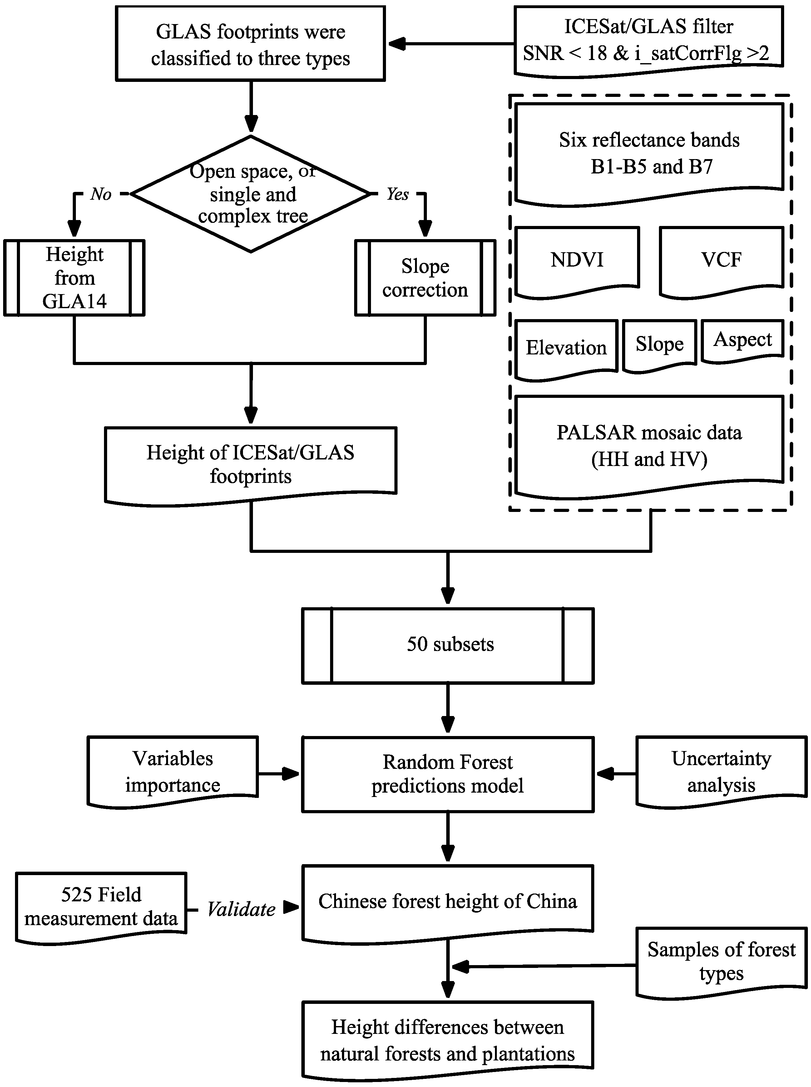
2.1. Height Extraction from Geoscience Laser Altimeter System (GLAS) Footprints

The ICESat/GLAS was launched on 12 January 2003. GLAS acquires data by transmitting a laser pulse with a duration of 10 nanoseconds and subsequently recording the pulse that is returned after being reflected from the footprint on the ground that is approximately 60 m in diameter [24]. GLAS data was acquired from the National Snow and Ice Data Center (NSIDC, http://nsidc.org/data/icesat), Release 33, focusing on the transmitted and received waveform data (GLA01), waveform parameterization data (GLA05) and Land surface altimetry data (GLA14). All of them were obtained from May to June 2006.

A three-step procedure was used to identify high-quality footprints and to extract their heights [25]. First, the footprints with low signal-to-noise (SNR < 18) and saturation (i_satCorrFlg > 2) were removed to reduce atmospheric attenuation, including could. Second, the GLAS footprints were classified to three types (open space, single tree or single layer building, and complex tree or multi-layer building) in terms of waveform indices derived from the GLAS original waveform [26]. Thirdly, for the first type (open space), which might include bare land, water, road, and sparse grassland, heights were derived from the GLA14 product. Due to the number restrictions in the returned waveform and the lack of slope correction in GLA14 product, the other two types (single tree or single layer building, and complex tree or multi-layer building) were processed with a Gaussian decomposition algorithm to extract returned waveforms from GLA01 and with a topographic correction factor (Equation (1)) to correct for the impact of topography on height extraction [27,28,29].

$$V{H}_{slope}=gpCntRng\left(1\right)-SigBeg-3\times \left({\sigma }_{gp}-{\sigma }_{transmit}\right)$$

(1)

where $V{H}_{slope}$ represents the vegetation height in the rugged area; in this study, a ‘rugged area’ is defined as a region with a slope greater than 5°, as determined by previous studies [13,27]. $gpCntRng\left(1\right)$ is the center position of the last peaks corresponding to the ground, $SigBeg$ represents the start of the earliest return peaks, corresponding to the presence of the forest canopy, ${\sigma }_{gp}$ represents the standard deviation of Gaussian decomposition from the ground peak, and ${\sigma }_{transmit}$ is defined as the standard deviation of Gaussian decomposition from a transmitted waveform.

GLAS spots overlaying with areas without vegetation (including bare land, impervious terrains, and water-rich regions) were identified and removed from the dataset with published land cover maps [30,31]. The final GLAS dataset contains 651,265 measurements of heights obtained from across China. The GLAS footprints were assigned to 50 ecozones of China for further modelling given that the similar climatic, geographic, and environmental condition in given ecozone [32]. The corresponding information of 50 ecozones is listed in the supporting Table S1.

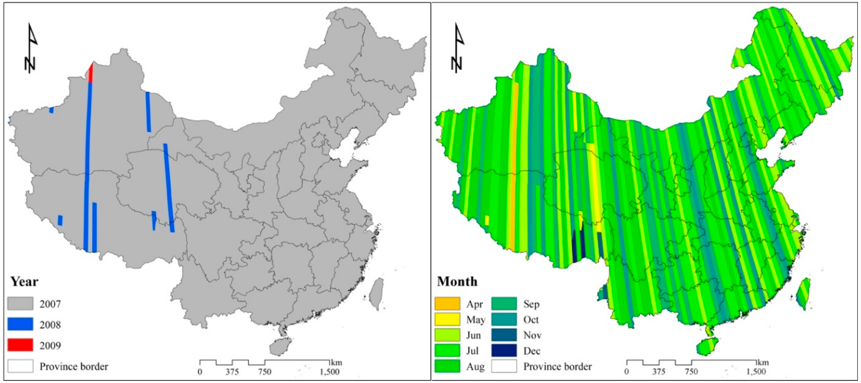
2.2. The Greenest Compositions from Landsat 5 Thematic Mapper (TM)

Landsat 5 Thematic Mapper (TM) images were obtained from the Google Earth Engine (GEE), and original images were obtained from the United States Geological Survey (USGS). We processed all available Landsat 5 TM standard surface reflectance data from 2006, including six reflectance bands B1-B5 and B7, as well as the cloud mask band. These surface reflectance data were processed using the LEDAPS method (http://ledaps.nascom.nasa.gov/, accessed on 6 August 2016), and data with cloud were processed using the Fmask algorithm [33]. We masked pixels from shadows and clouds in the mask band. Then, we calculated the Normalized Difference Vegetation Index (NDVI) for all available Landsat 5 TM data obtained in 2006. Pixels with maximum NDVI in 2006 were selected to represent the greenest compositions recorded in 2006, which relate to data from the growing season. The final ‘greenest composition’ thus includes six reflectance bands from Landsat 5 TM and NDVI.

2.3. Landsat Vegetation Continuous Fields (VCF) Tree Cover and Topographic Data

Vegetation continuous fields (VCF) data represent the percentage of a pixel’s area covered by woody vegetation greater than 5 m in height at a resolution of 30 m. These data are derived from all seven bands of Landsat 5 TM and Landsat 7 ETM+; these datasets have been produced in 2000, 2005 and 2010 [34]. In this study, because our Landsat 5 TM images and GLAS data were obtained close to 2005, we use VCF data obtained in 2005.

Shuttle Radar Topography Mission (SRTM) digital elevation model (DEM) data, which also have a spatial resolution of 30 m, were released in 2015. This dataset underwent a void-filling process [35,36] in which its elevations, slopes, and other aspects [37] were extracted as input variables for subsequent modeling.

2.4. Phased Array L-Band Synthetic Aperture Radar (PALSAR-2/PALSAR) Mosaic Dataset

The Phased Array L-band Synthetic Aperture Radar (PALSAR) yearly mosaic dataset was collected globally from 2007 to 2010. It has a resolution of 25 m and was aggregated from PALSAR located on the Advanced Land Observing Satellite (ALOS) [38]. Original SAR data were obtained using the fine beam dual polarization mode (FBD), which utilizes HH (horizontal-transmit, horizontal receive) and HV (horizontal-transmit, vertical receive). Geometric distortion of these images and topographic effects on the images’ intensities were reduced with an estimated geometric accuracy of 12 m [39]. Original images recording a minimum response to surface moisture were selected and composited to the mosaic dataset, which was then radiometrically calibrated and stored as digital numbers (DN). These DN values can be converted to gamma naught values (representing the backscattering coefficient), which are expressed in decibel units (dB), using the following equation [40]:

$${\gamma }^{°}=10lo{g}_{10}\langle D{N}^2\rangle +CF$$

(2)

where CF represents a calibration factor equal to −83.0 dB, and < > represents the ensemble averaging.

We downloaded all PALSAR HH and HV data acquired in 2007 because it is the closest year to the times our optical and GLAS data were collected. Then we converted these data into backscattering coefficients (in decibels). We also selected PALSAR data from the growing season and from closer years in cases of limited availability in 2007 (Figure 1). To achieve consistency between datasets, HH and HV data were resampled to acquire a resolution of 30 m with a nearest neighbor interpolation.

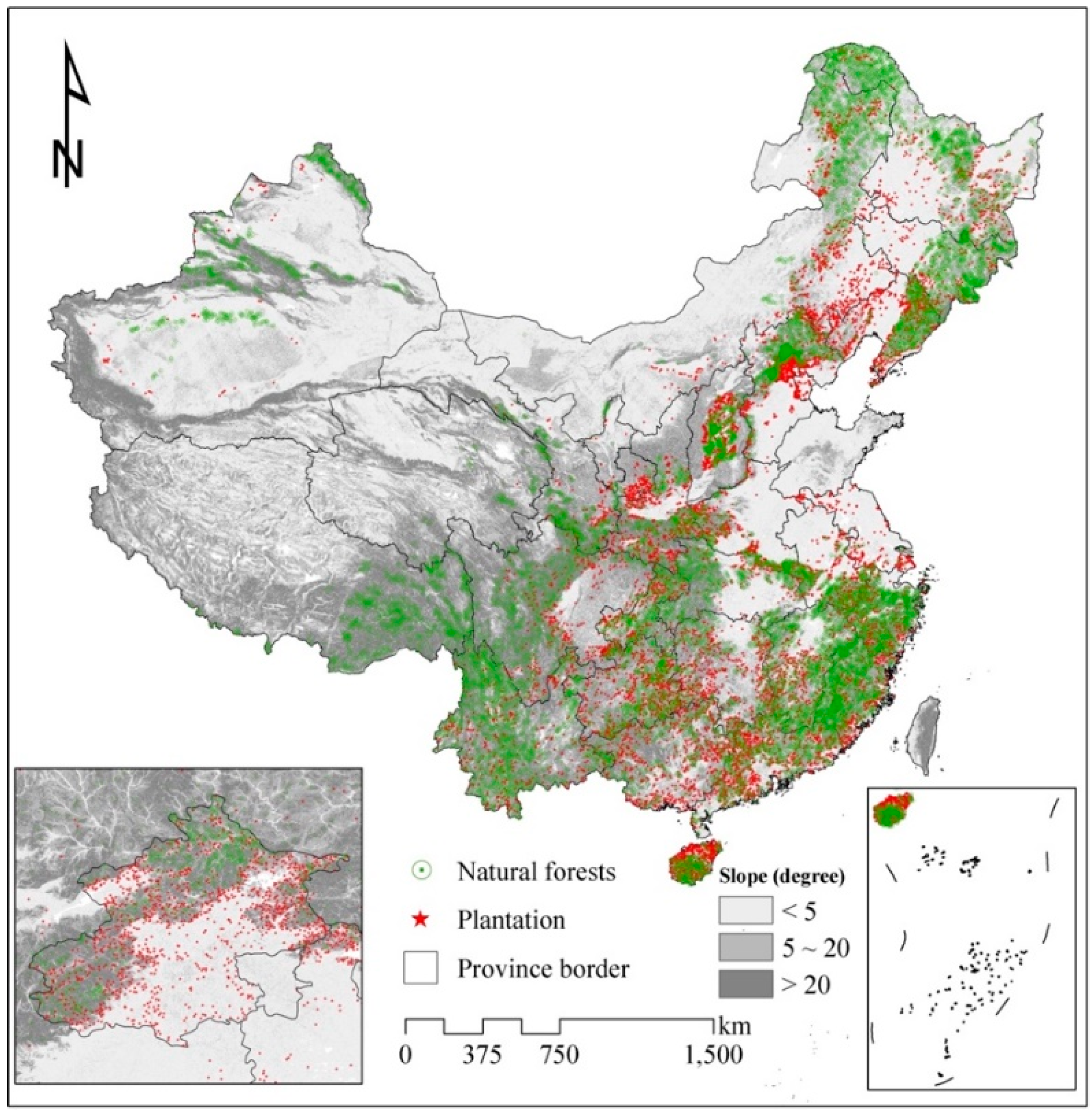
2.5. Sampling Selection for Natural Forests and Plantations

The State Forestry Bureau of China generates and examines the National Forestry Inventories dataset (NFI), which compiles data concerning the areas, types, origins and distributions of forest resources [4]. Survey samples are systematically allocated according to statistical principles, and investigators periodically revisit survey sample sites. For example, the NFI has a 5-year cycle of survey site visits, and approximately 20% of provinces conduct inventories each year. Therefore, national statistics were thus obtained by summing all statistical data from all provinces acquired in a 5-year cycle. Through this sampling, the overall accuracy of these results was assessed to be approximately 95% [41]. We interpreted the forest origins (natural forest or plantations) of these samples at the province scale by using the current forest map of the eighth NFI (2009–2013). In total, 9772 samples were interpreted from the Atlas of Forest Resources of China to have originated from natural forests, and 5010 samples were deemed likely to have originated from plantations (Figure 2). Moreover, forest types for natural forest and plantations were interpreted as natural conifer forests (NCF), natural broadleaf forests (NBF), natural conifer and broadleaf mixed forests (NMF), natural bamboo forests (NB), conifer plantations (CP), broadleaf plantations (BLP), conifer and broadleaf mixed plantations (MP) and bamboo plantations (BP).

2.6. Wall-to-Wall Forest Height Estimation

In order to model spatially continuous forest heights, GLAS height data were used as training data and related to the data from seven Landsat 5 TM variables (B1–B5, B7 and NDVI), two PALSAR mosaic data (HH and HV), three SRTM-derived metrics (elevation, slope and aspect) and VCF with the random forest (RF) regression tree (Figure 3), given its ability to handle a great deal of input predictors that are not independent and non-linearly separable [42,43,44,45].

Using an RF regression tree to produce spatial modeling involves two main steps: first, determining the optimal parameters for the training of the RF regression tree, and second, producing gridded forest heights using RF regression tree. These training and modeling processes were implemented one ecozone at a time. Both the number of trees and the number of variables to split on each node were determined iteratively [46]; the initial value for the number of trees was set at 100 and the initial value for the number of nodes was set at 3. The iterative test was programmed to stop if the predicted height showed a strong correlation with the height measured from its corresponding GLAS footprint in the cross validation dataset, or if the values of trees and nodes reached 500 (using an interval of 100) and 7 (using an interval of 1), respectively. The importance of the 13 input predictors was estimated based on an out-of-bag error estimate [46]. After an ensemble decision tree was built into the training procedure, the rules of each decision tree, along with two optimal parameters, were used to predict height in areas without GLAS footprints. Finally, heights from non-forested areas were masked with previous forest classification data [47].

2.7. Assessment of Accuracy and Prediction of Uncertainty

Since the NFI only provides general information, such as forest type, forest area and origins at provincial level and does not provide forest height at plot scale [48], we collected 525 forest height measurements to estimate the accuracy of the modeled wall-to-wall forest heights. The distribution of these measurements is illustrated in Figure 4. This dataset includes the main tree species across China, including locust, eucalyptus, polar, Korean pine, larch, birch, mason pine, Chinese fir, and spruce. 435 measurements were obtained from peer-reviewed Chinese journals and 90 measurements were collected from national forest inventories [49]. Each plot was at least 0.05 ha in size, and the mean height of dominant trees from the emergent layer and the canopy layer in each plot was recorded. To reduce the difference between the mean tree height of our collected data and the modeled forest canopy height from remote sensing data, the plots belongs to mature forest or relatively uniform growing forests were selected in terms of the screening criteria in a previous study [27].

A regression through the origin (RTO) analysis was used to calculate the degree of correlation between the height data measured in the field and the predicted forest heights [50]. The coefficient of determination (R²) and root mean square error (RMSE) are used to quantify the accuracy of this correlation. MAE also calculated to check the bias between the field measured heights and the modeled forest heights, considering the regression analysis is sensitive to data region.

The uneven spatial distribution and gaps among GLAS footprints would affect wall-to-wall forest height mapping accuracy in the course of extrapolating forest heights in areas without corresponding GLAS footprints. To quantify this uncertainty or variance (${\epsilon }_{GLAS}$), we randomly picked up 10 subsets of GLAS footprints which comprising from 55% to 100% of the whole GLAS footprints (with a 5% interval, e.g., 55%, 60%, 65%, …, 95%, 100%). Ten forest heights were then modeled with the 10 GLAS footprints subsets by running the RF regression tree. The deviation (within ten forest heights) was then calculated to indicate the uncertainty associated with the uneven spatial distribution of GLAS footprints:

$${\epsilon }_{GLAS}=\sqrt{\frac{{{\displaystyle \sum }}_{i=1}^{10}{\left(\widehat{H_i}-\overline{H}\right)}^2}{10}}$$

(3)

where $\widehat{H_i}$ is the predicted forest height at the ith iteration and $\overline{H}$ is the average of all predicted forest heights.

To quantify the performance of PALSAR data on large scale forest heights estimation, we calculate the accuracy (RMSE and R²) and uncertainty (${\epsilon }_{GLAS}$) after and before integrating PALSAR data.

3. Results and Discussion

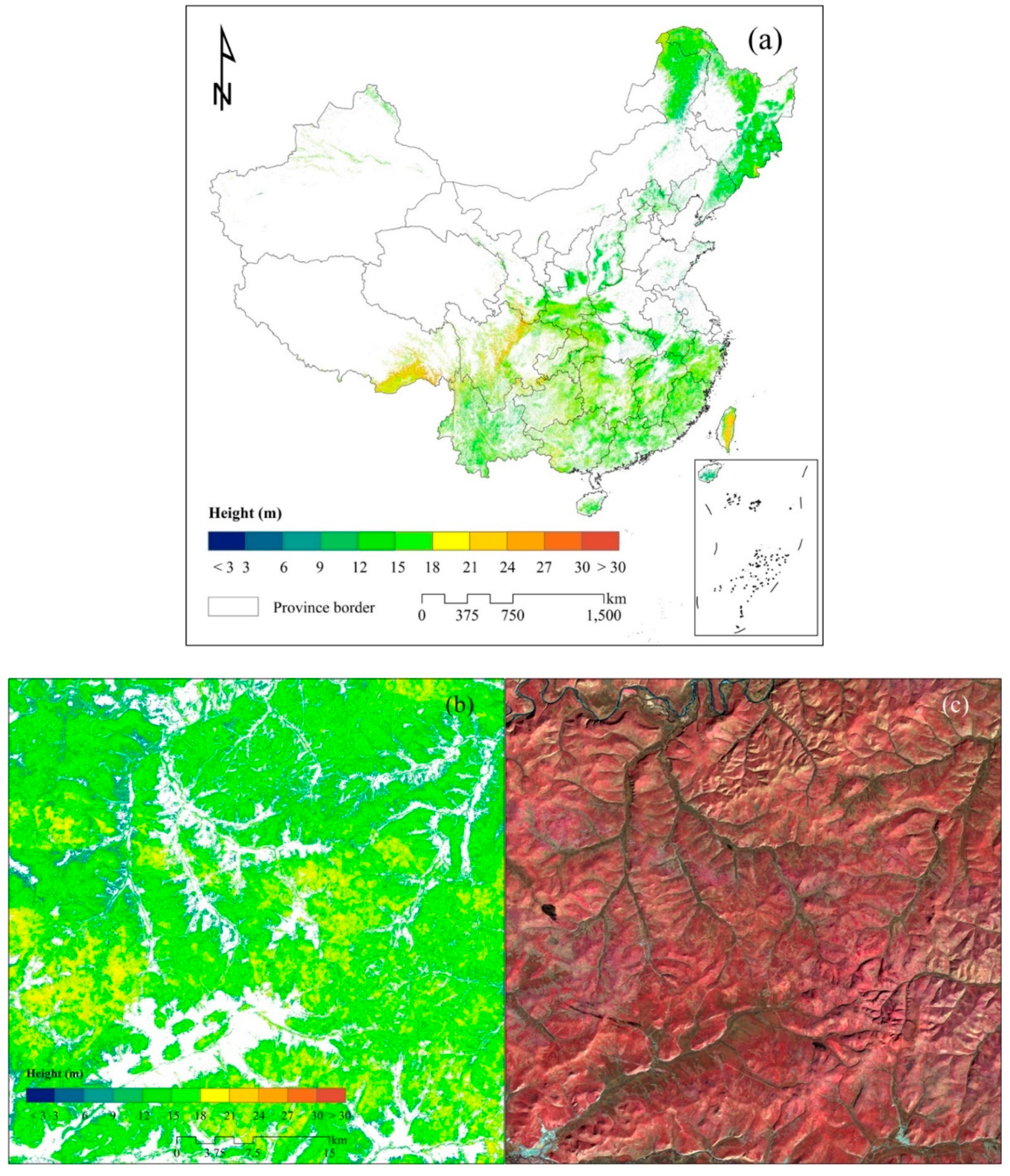
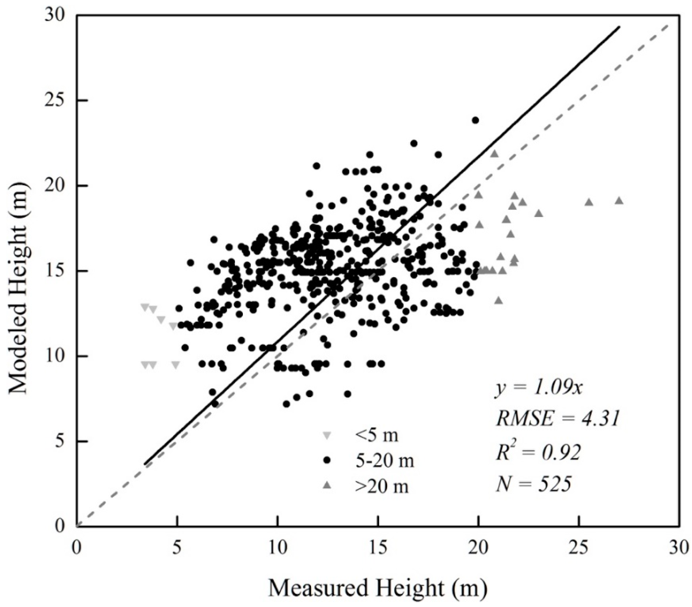
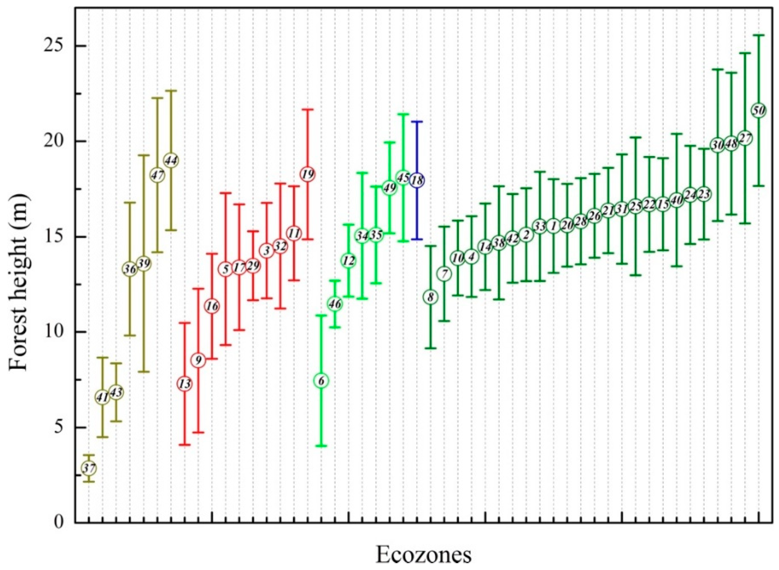
3.1. Accuracy and Spatial Patterns of Forest Height in China

The modeled wall-to-wall forest heights, as shown in Figure 5, have a linear correlation with the 525 in situ measured forest heights, yielding an R² value of 0.92 and an RMSE value of 4.31 m with regression through the origin, and with an overall MAE for height estimation of 3.87 m. Compared with field measurement, low (<5 m) and high (>20 m) forest heights show over and under estimations, respectively (Figure 6). The modeled forest heights in China range from 1.41–38.94 m, with an average forest height of 16.08 m, a median forest height of 15.78 m and a standard deviation of 3.34 m. In general, regions of maximum forest height in China (mean heights > 20 m) include the regions of southeast Tibet which are occupied by tropical rainforests and monsoon forests, the conifer forests of the Sichuan, and the tropical forests, rainforests, and evergreen broadleaf forests of Taiwan. The region with the minimum forest height (mean height < 3 m) is located in western Inner Mongolia. Forest height in northeast China, considered to be a major forest resource base, is 14.42 ± 2.37 m. Additionally, forest heights vary among 50 different ecozones (Figure 7). For example, the mean forest height in forest-dominated ecozones is 16.25 ± 2.77 m, which is larger than the mean forest height of 13.05 ± 2.91 m recorded in other ecozones. The statistical information about minimum, maximum, 10th and 90th percentiles, median mean, standard deviation (SD) of forest height in 50 ecozones, is listed in supplement Table S2.

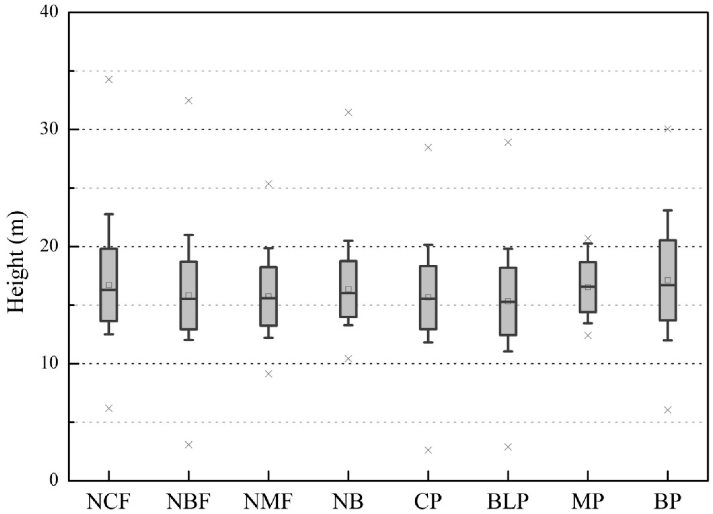
3.2. Height Differences between Natural Forests and Plantations

Analysis of these samples indicates that natural forests have a mean height of 16.17 ± 2.94 m (N = 9772), whereas plantations have a mean height of 15.60 ± 2.82 m (N = 5010). Therefore, these samples suggest that natural forests and plantations have similar mean heights. These mean heights vary only slightly between different forest types (Figure 8): the greatest mean heights are seen in natural conifer forests (NCF: 16.72 ± 3.10 m), followed by natural bamboo forests (NB: 16.37 ± 2.40 m), natural broadleaf forests (NBF: 15.83 ± 2.89 m), and natural conifer and broadleaf mixed forests (NMF: 15.75 ± 2.51 m). Within plantations, the greatest mean heights are seen in bamboo plantations (17.13 ± 3.43 m), followed by conifer and broadleaf mixed plantations (MP: 16.54 ± 2.13 m), conifer plantations (CP: 15.64 ± 2.70 m), and broadleaf plantations (BP: 15.53 ± 2.89 m).

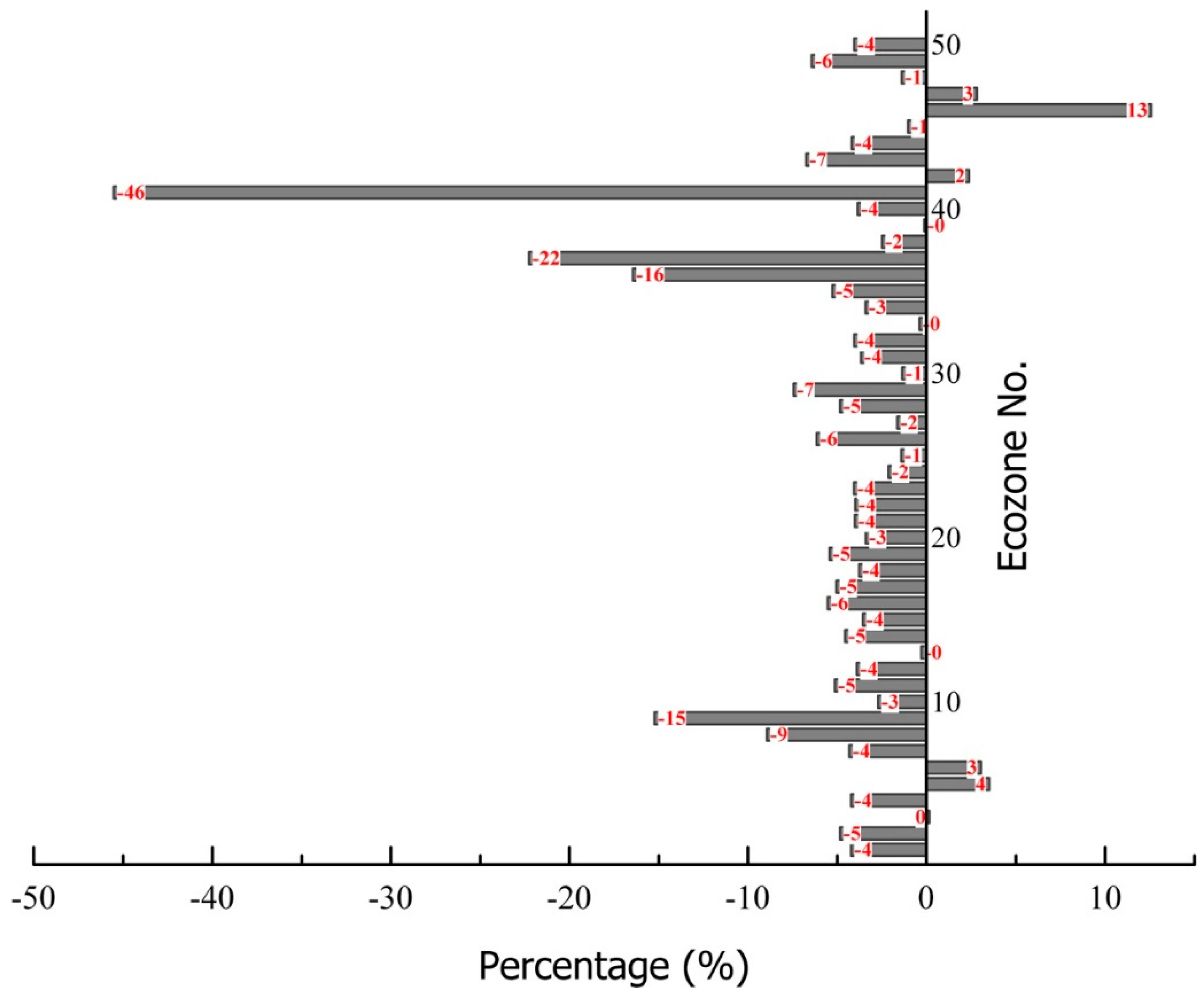
3.3. Improvement after Integrating PALSAR Data

The integration of PALSAR data caused the RMSE to decrease from 4.57 m to 4.31 m and the R² to increase from 0.90 to 0.92 when compared with forest heights without PALSAR data, and the uncertainty (${\epsilon }_{GLAS}$) decreased by an average of 4.58% at the ecozone level (Figure 9). Desert-dominated ecozones recorded the greatest decrease in uncertainty (−45.53%). Meanwhile, uncertainties decreased in all forest-dominated ecozones. Contrastingly, combining PALSAR data slightly increased the uncertainty in six ecozones, with the greatest increase in uncertainty (12.58%) recorded in grassland-dominated ecozones. Previous studies have demonstrated that SAR is useful for estimating forest biomass [51], but few have suggested that PALSAR can be used to estimate forest height. The results of this study demonstrate that PALSAR can improve the accuracy of forest height estimations. García et al., have also reported that including PALSAR for estimating forest height improved the estimation accuracy, and this improvement depends on the vegetation type and structure [52]. Although the improvement of R² and RMSE in our study is not obvious when considering all ecozones together, we also found that the importance of PALSAR varies with forest types and structure among the sub zones.

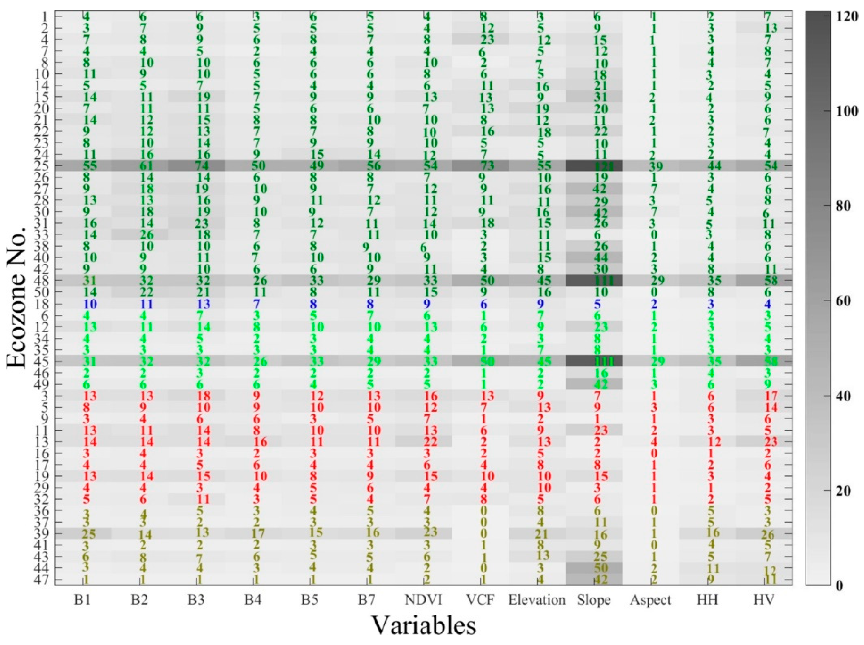
3.4. Importance of Predictors to Model Wall-to-Wall Forest Height

The importance of these 13 predictors varies between different sub zones, as is shown in Figure 10, which emphasizes the importance of a given predictor by the darkness of the variable and the size of its value. In general, the most important metric for modeling gridded forest height is the slope derived from the SRTM, except in ecozones dominated by agricultural ecosystems. Aspect and HH are the least important predictors, and the HV metric is more important in non-forest-dominated ecozones than it is in forest-dominated ecozones. Predictors such as surface reflectance of the red band, HV backscatter, and slope are more important than other Landsat- and PALSAR-related metrics and SRTM-derived metrics. In particular, red band outperformed than other bands from Landsat, which conformed to previous study that employed time series Landsat images to map forest height in Sub-Saharan Africa [53]. Differences in variables’ importance between the sub zones could be explained by forest types and their structural characters in different biomes, such as crown diameter, distance between trees, tree positioning, stand age and LAI. Moreover, determining the relative importance of these predictors can help improve future computational efficiency by allowing researchers to acquire important data for nationwide or worldwide forest-height modeling.

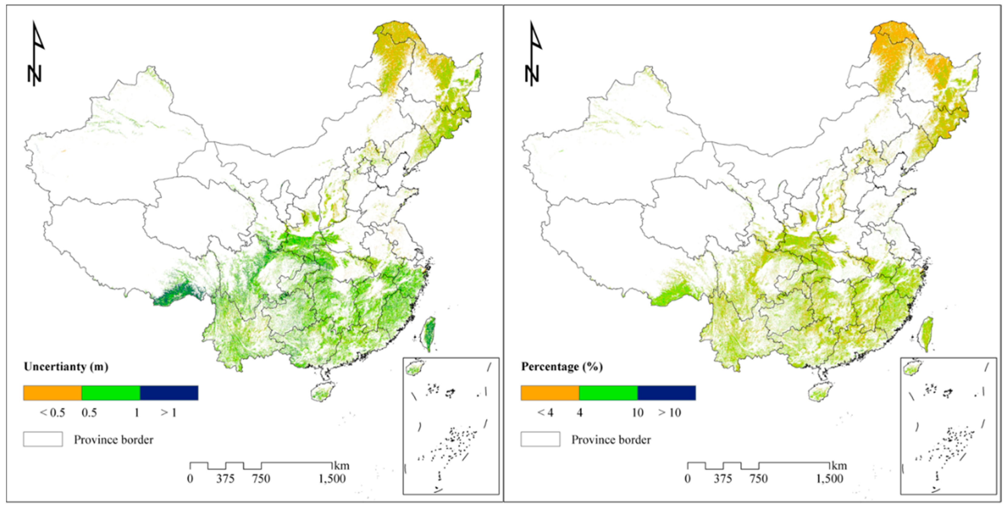
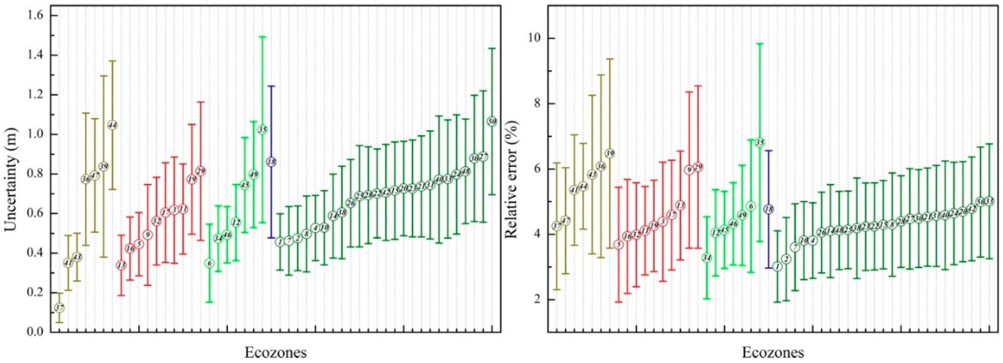
3.5. Quantifying Uncertainty Caused by Footprints Space in Modeled Forest Heights

The uncertainty (${\epsilon }_{GLAS}$) induced by the spatial gaps among GLAS footprints in predicting wall-to-wall forest height varies from 0.026–4.43 m, with a mean uncertainty of 0.64 m (Figure 11). This uncertainty can result in differences between in situ measured forest heights and their corresponding modeled heights, and consideration of this uncertainty reduced the RMSE from 4.40 m to 4.31 m. Forests in southeast Tibet and Taiwan, which have the greatest mean forest heights, contribute the most to this uncertainty (>1 m), whereas forests in Northeast China contribute the least (<0.5 m). When comparing the spatial patterns of forest heights and their uncertainties, it becomes apparent that uncertainty increases with increasing mean forest height in these ecozones. At the pixel scale, the relative error caused by this uncertainty (defined as the percentage of predicted average forest heights that are encompassed by a given uncertainty) has been estimated to be 3.97 ± 1.44% (Figure 11). Additionally, forest-dominated ecozones yield lower relative errors than non-forest-dominated ecozones (Figure 12). According to the standards of China’s NFI, the uncertainty of a tree height measurement should not be greater than 5% [4]. More than 80% (82.59%) of analyzed pixels yield a relative error of less than 5% in this finer-resolution forest height map. To further improve the accuracy of forest height measurements in China, future research should focus on regions with large uncertainties or relative errors, such as southeast Tibet.

3.6. Comparisons with Published Forest Heights

We compared the forest heights presented here with previous forest heights obtained by remote sensing mapping and field measurements. Nationwide field datasets have a mean tree height of ~10 m [54], which is less than the mean forest height reported in our study (16.08 m). This difference might be caused by the limited number of forest plots used in the field datasets. For example, the above nationwide field datasets have included field measurement datasets of approximately 1500 plots, from which mean forest heights are generated by applying statistics through these random samples. However, the modeled mean forest height is dominant canopy height at the pixel scale. This inconsistency causes differences between field data and the forest height generated in this study. Another study used 1 km remote sending data to calculate a mean height of 36.44 m [16], which is much larger than both our results and the nationwide field datasets. The difference between these two forest heights can be explained by the fact that this study was undertaken in the mountainous regions of southeast and northeast Tibet, whereas we used a different slope-correction for GLAS height extraction. This difference could also be caused by differences in the source and scale of the remote-sensing data. Although the differences imply that forest height mapping is still a challenge, our modeled forest heights show good agreement with independent field measurements. Future work should reduce the uncertainty of forest height mapping with more field plots and new LiDAR data.

4. Conclusions

In this study, we developed a new forest height map by integrating results from multiple sources of remote-sensing data, including ICESat/GLAS, LandSat 5 TM, SRTM and PALSAR. Our modeled forest heights vary from 1.41–38.94 m across China, with an average Chinese forest height of 16.08 m and a standard deviation of 3.34 m. These results yield estimated R² and RMSE values of 0.92 and 4.31 m, respectively, when compared with 525 field-measured forest heights. Mean forest heights differ only slightly among different forest types, with natural forests recording mean heights of 16.17 ± 2.94 m and plantations recording mean heights of 15.60 ± 2.82 m.

The uncertainty caused by the distribution of GLAS footprints was estimated to be 0.64 m. Integrating this uncertainty into the model reduced the RMSE from 4.40 m to 4.31 m. Additionally, more than 80% (82.59%) of pixels yielded a relative error of less than 5%. This low relative error implies that the forest heights derived from GLAS footprints can potentially be used to detect changes in forest height.

Integrating PALSAR data into this model increased the accuracy of forest height estimates, especially in forest-dominated ecozones; the average uncertainty decreased by 4.58%. It also demonstrated that, in forest-height modeling, HV backscatter is more important than HH backscatter.

Currently, forest-height measurements in China have the greatest uncertainties in southeast and northeast Tibet. Therefore, future efforts should focus on integrating new LiDAR data, SAR/InSAR data, and additional field plots to reduce the uncertainties in these areas.

References

1. Gong, P. Remote sensing of environmental change over China: A review. Chin. Sci. Bull. 2012, 57, 2793–2801. [Google Scholar] [CrossRef] [Green Version]
2. Pettorelli, N.; Wegmann, M.; Skidmore, A.; Mücher, S.; Dawson, T.P.; Fernandez, M.; Lucas, R.; Schaepman, M.E.; Wang, T.; O’Connor, B.; et al. Framing the concept of satellite remote sensing essential biodiversity variables: Challenges and future directions. Remote Sens. Ecol. Conserv. 2016, 2, 122–131. [Google Scholar] [CrossRef]
3. Bontemps, S.D.P.; Van Bogaert, E.; Arino, O.; Kalogirou, V.; Ramos, P.; Jose, J. GLOBCOVER 2009 Products Description and Validation Report; Université catholique de Louvain (UCL) & European Space Agency (esa): Louvain-la-Neuve, Belgium, 2011. [Google Scholar]
4. Zeng, W.; Tomppo, E.; Healey, S.; Gadow, K. The national forest inventory in China: History-results-international context. For. Ecosyst. 2015, 2, 23. [Google Scholar] [CrossRef]
5. Zhang, P.; Shao, G.; Zhao, G.; Le Master, D.C.; Parker, G.R.; Dunning, J.B.; Li, Q. China’s Forest Policy for the 21st Century. Science 2000, 288, 2135–2136. [Google Scholar] [CrossRef] [PubMed]
6. Lefsky, M.A.; Cohen, W.B.; Parker, G.G.; Harding, D.J. LiDAR Remote Sensing for Ecosystem Studies. Bioscience 2002, 52, 19–30. [Google Scholar] [CrossRef]
7. Asner, G.P.; Knapp, D.E.; Kennedy-Bowdoin, T.; Jones, M.O.; Martin, R.E.; Boardman, J.; Field, C.B. Carnegie Airborne Observatory: In-flight fusion of hyperspectral imaging and waveform light detection and ranging (wLiDAR) for three-dimensional studies of ecosystems. J. Appl. Remote Sens. 2007, 1, 013536. [Google Scholar] [CrossRef]
8. Zwally, H.J.; Schutz, B.; Abdalati, W.; Abshire, J.; Bentley, C.; Brenner, A.; Bufton, J.; Dezio, J.; Hancock, D.; Harding, D.; et al. ICESat’s laser measurements of polar ice, atmosphere, ocean, and land. J. Geodyn. 2002, 34, 405–445. [Google Scholar] [CrossRef]
9. Sun, G.; Ranson, K.J.; Guo, Z.; Zhang, Z.; Montesano, P.; Kimes, D. Forest biomass mapping from lidar and radar synergies. Remote Sens. Environ. 2011, 115, 2906–2916. [Google Scholar] [CrossRef] [Green Version]
10. Wang, X.; Cheng, X.; Gong, P.; Huang, H.; Li, Z.; Li, X. Earth science applications of ICESat/GLAS. Int. J. Remote Sens. 2011, 32, 8837–8864. [Google Scholar] [CrossRef]
11. Schutz, B.E.; Zwally, H.J.; Shuman, C.A.; Hancock, D.; DiMarzio, J.P. Overview of the ICESat Mission. J. Geophys. Res. 2005, 32, L21S01. [Google Scholar] [CrossRef]
12. Lefsky, M.A. A global forest canopy height map from the Moderate Resolution Imaging Spectroradiometer and the Geoscience Laser Altimeter System. Geophys. Res. Lett. 2010, 37, L15401. [Google Scholar] [CrossRef]
13. Simard, M.; Pinto, N.; Fisher, J.B.; Baccini, A. Mapping forest canopy height globally with spaceborne lidar. J. Geophys. Res. Biogeosci. 2011, 116, G04021. [Google Scholar] [CrossRef]
14. Wang, Y.; Li, G.; Ding, J.; Guo, Z.; Tang, S.; Wang, C.; Huang, Q.; Liu, R.; Chen, J.M. A combined GLAS and MODIS estimation of the global distribution of mean forest canopy height. Remote Sens. Environ. 2016, 174, 24–43. [Google Scholar] [CrossRef]
15. Los, S.O.; Rosette, J.A.B.; Kljun, N.; North, P.R.J.; Chasmer, L.; Suárez, J.C.; Hopkinson, C.; Hill, R.A.; van Gorsel, E.; Mahoney, C.; et al. Vegetation height and cover fraction between 60° S and 60° N from ICESat GLAS data. Geosci. Model Dev. 2012, 5, 413–432. [Google Scholar] [CrossRef]
16. Ni, X.; Zhou, Y.; Cao, C.; Wang, X.; Shi, Y.; Park, T.; Choi, S.; Myneni, R. Mapping Forest Canopy Height over Continental China Using Multi-Source Remote Sensing Data. Remote Sens. 2015, 7, 8436–8452. [Google Scholar] [CrossRef] [Green Version]
17. Scarth, P.; Armston, J.; Lucas, R.; Bunting, P. A Structural Classification of Australian Vegetation Using ICESat/GLAS, ALOS PALSAR, and Landsat Sensor Data. Remote Sens. 2019, 11, 147. [Google Scholar] [CrossRef]
18. Tao, S.; Guo, Q.; Li, C.; Wang, Z.; Fang, J. Global patterns and determinants of forest canopy height. Ecology 2016, 97, 3265–3270. [Google Scholar] [CrossRef]
19. Axelsson, S.R.J.; Eriksson, M.; Halldin, S. Tree-heights derived from radar profiles over boreal forests. Agric. For. Meteorol. 1999, 98, 427–435. [Google Scholar] [CrossRef]
20. Hall, F.G.; Bergen, K.; Blair, J.B.; Dubayah, R.; Houghton, R.; Hurtt, G.; Kellndorfer, J.; Lefsky, M.; Ranson, J.; Saatchi, S.; et al. Characterizing 3D vegetation structure from space: Mission requirements. Remote Sens. Environ. 2011, 115, 2753–2775. [Google Scholar] [CrossRef] [Green Version]
21. Thiel, C.; Schmullius, C. The potential of ALOS PALSAR backscatter and InSAR coherence for forest growing stock volume estimation in Central Siberia. Remote Sens. Environ. 2016, 173, 258–273. [Google Scholar] [CrossRef]
22. Mitchard, E.T.A.; Saatchi, S.S.; Woodhouse, I.H.; Nangendo, G.; Ribeiro, N.S.; Williams, M.; Ryan, C.M.; Lewis, S.L.; Feldpausch, T.R.; Meir, P. Using satellite radar backscatter to predict above-ground woody biomass: A consistent relationship across four different African landscapes. Geophys. Res. Lett. 2009, 36, L23401. [Google Scholar] [CrossRef]
23. Joshi, N.; Mitchard, E.; Schumacher, J.; Johannsen, V.; Saatchi, S.; Fensholt, R. L-Band SAR Backscatter Related to Forest Cover, Height and Aboveground Biomass at Multiple Spatial Scales across Denmark. Remote Sens. 2015, 7, 4442–4472. [Google Scholar] [CrossRef] [Green Version]
24. Harding, D.J.; Carabajal, C.C. ICESat waveform measurements of within-footprint topographic relief and vegetation vertical structure. J. Geophys. Res. 2005, 32, L21S10. [Google Scholar] [CrossRef]
25. Huang, H.; Liu, C.; Wang, X.; Biging, G.S.; Chen, Y.; Yang, J.; Gong, P. Mapping vegetation heights in China using slope correction ICESat data, SRTM, MODIS-derived and climate data. ISPRS J. Photogramm. Remote Sens. 2017, 129, 189–199. [Google Scholar] [CrossRef]
26. Liu, C.; Huang, H.; Gong, P.; Wang, X.; Wang, J.; Li, W.; Li, C.; Li, Z. Joint Use of ICESat/GLAS and Landsat Data in Land Cover Classification: A Case Study in Henan Province, China. IEEE J. Sel. Top. Appl. Earth Obs. Remote Sens. 2015, 8, 511–522. [Google Scholar] [CrossRef]
27. Wang, X.; Huang, H.; Gong, P.; Liu, C.; Li, C.; Li, W. Forest Canopy Height Extraction in Rugged Areas With ICESat/GLAS Data. IEEE Trans. Geosci. Remote Sens. 2014, 52, 4650–4657. [Google Scholar] [CrossRef]
28. Gong, P.; Li, Z.; Huang, H.; Sun, G.; Wang, L. ICESat GLAS Data for Urban Environment Monitoring. IEEE Trans. Geosci. Remote Sens. 2011, 49, 1158–1172. [Google Scholar] [CrossRef]
29. Huang, H.; Liu, C.; Wang, X.; Zhou, X.; Gong, P. Integration of multi-resource remotely sensed data and allometric models for forest aboveground biomass estimation in China. Remote Sens. Environ. 2019, 221, 225–234. [Google Scholar] [CrossRef]
30. Arino, O.; Ramos Perez, J.J.; Kalogirou, V.; Bontemps, S.; Defourny, P.; Van Bogaert, E. Global land cover map for 2009 (GlobCover 2009). In Proceedings of the ESA Living Planet Symposium, Bergen, Norway, 28 June–2 July 2010. [Google Scholar]
31. Gong, P.; Wang, J.; Yu, L.; Zhao, Y.; Zhao, Y.; Liang, L.; Niu, Z.; Huang, X.; Fu, H.; Liu, S.; et al. Finer resolution observation and monitoring of global land cover: First mapping results with Landsat TM and ETM+ data. Int. J. Remote Sens. 2013, 34, 2607–2654. [Google Scholar] [CrossRef]
32. Fu, B.J.; Liu, G.H.; Lü, Y.H.; Chen, L.D.; Ma, K.M. Ecoregions and ecosystem management in China. Int. J. Sustain. Dev. World Ecol. 2004, 11, 397–409. [Google Scholar] [CrossRef]
33. Zhu, Z.; Wang, S.; Woodcock, C.E. Improvement and expansion of the Fmask algorithm: Cloud, cloud shadow, and snow detection for Landsats 4–7, 8, and Sentinel 2 images. Remote Sens. Environ. 2015, 159, 269–277. [Google Scholar] [CrossRef]
34. Sexton, J.O.; Song, X.-P.; Feng, M.; Noojipady, P.; Anand, A.; Huang, C.; Kim, D.-H.; Collins, K.M.; Channan, S.; DiMiceli, C.; et al. Global, 30-m resolution continuous fields of tree cover: Landsat-based rescaling of MODIS vegetation continuous fields with lidar-based estimates of error. Int. J. Digit. Earth 2013, 6, 427–448. [Google Scholar] [CrossRef] [Green Version]
35. Reuter, H.I.; Nelson, A.; Jarvis, A. An evaluation of void-filling interpolation methods for SRTM data. Int. J. Geogr. Inf. Sci. 2007, 21, 983–1008. [Google Scholar] [CrossRef]
36. Farr, T.G.; Rosen, P.A.; Caro, E.; Crippen, R.; Duren, R.; Hensley, S.; Kobrick, M.; Paller, M.; Rodriguez, E.; Roth, L.; et al. The Shuttle Radar Topography Mission. Rev. Geophys. 2007, 45, RG2004. [Google Scholar] [CrossRef]
37. Moore, I.D.; Grayson, R.B.; Ladson, A.R. Digital terrain modelling: A review of hydrological, geomorphological, and biological applications. Hydrol. Process. 1991, 5, 3–30. [Google Scholar] [CrossRef]
38. Shimada, M.; Itoh, T.; Motooka, T.; Watanabe, M.; Shiraishi, T.; Thapa, R.; Lucas, R. New global forest/non-forest maps from ALOS PALSAR data (2007–2010). Remote Sens. Environ. 2014, 155, 13–31. [Google Scholar] [CrossRef]
39. Qin, Y.; Xiao, X.; Dong, J.; Zhang, G.; Shimada, M.; Liu, J.; Li, C.; Kou, W.; Moore, B., III. Forest cover maps of China in 2010 from multiple approaches and data sources: PALSAR, Landsat, MODIS, FRA, and NFI. ISPRS J. Photogramm. Remote Sens. 2015, 109, 1–16. [Google Scholar] [CrossRef] [Green Version]
40. Shimada, M.; Isoguchi, O.; Tadono, T.; Isono, K. PALSAR Radiometric and Geometric Calibration. IEEE Trans. Geosci. Remote Sens. 2009, 47, 3915–3932. [Google Scholar] [CrossRef]
41. Chinese Ministry of Forestry. Forest Resource Report of China for Periods 2009–2013; Department of Forest Resource and Management, Chinese Ministry of Forestry: Beijing, China, 2014. [Google Scholar]
42. Van Beijma, S.; Comber, A.; Lamb, A. Random forest classification of salt marsh vegetation habitats using quad-polarimetric airborne SAR, elevation and optical RS data. Remote Sens. Environ. 2014, 149, 118–129. [Google Scholar] [CrossRef]
43. Belgiu, M.; Drăguţ, L. Random forest in remote sensing: A review of applications and future directions. ISPRS J. Photogramm. Remote Sens. 2016, 114, 24–31. [Google Scholar] [CrossRef]
44. Huang, H.; Chen, Y.; Clinton, N.; Wang, J.; Wang, X.; Liu, C.; Gong, P.; Yang, J.; Bai, Y.; Zheng, Y.; et al. Mapping major land cover dynamics in Beijing using all Landsat images in Google Earth Engine. Remote Sens. Environ. 2017, 202, 166–176. [Google Scholar] [CrossRef]
45. Gong, P.; Liu, H.; Zhang, M.; Li, C.; Wang, J.; Huang, H.; Clinton, N.; Ji, L.; Li, W.; Bai, Y.; et al. Stable classification with limited sample: transferring a 30-m resolution sample set collected in 2015 to mapping 10-m resolution global land cover in 2017. Sci. Bull. 2019, 64, 370–373. [Google Scholar] [CrossRef] [Green Version]
46. Breiman, L. Random Forests. Mach. Learn. 2001, 45, 5–32. [Google Scholar] [CrossRef] [Green Version]
47. Li, C.; Wang, J.; Hu, L.; Yu, L.; Clinton, N.; Huang, H.; Yang, J.; Gong, P. A Circa 2010 Thirty Meter Resolution Forest Map for China. Remote Sens. 2014, 6, 5325–5343. [Google Scholar] [CrossRef] [Green Version]
48. Piao, S.; Fang, J.; Zhu, B.; Tan, K. Forest biomass carbon stocks in China over the past 2 decades: Estimation based on integrated inventory and satellite data. J. Geophys. Res. Biogeosci. 2005, 110, G01006. [Google Scholar] [CrossRef]
49. Zhang, C.; Ju, W.; Chen, J.M.; Zan, M.; Li, D.; Zhou, Y.; Wang, X. China’s forest biomass carbon sink based on seven inventories from 1973 to 2008. Clim. Chang. 2013, 118, 933–948. [Google Scholar] [CrossRef]
50. Eisenhauer, J.G. Regression through the Origin. Teach. Stat. 2003, 25, 76–80. [Google Scholar] [CrossRef]
51. Chowdhury, T.A.; Thiel, C.; Schmullius, C. Growing stock volume estimation from L-band ALOS PALSAR polarimetric coherence in Siberian forest. Remote Sens. Environ. 2014, 155, 129–144. [Google Scholar] [CrossRef]
52. García, M.; Saatchi, S.; Ustin, S.; Balzter, H. Modelling forest canopy height by integrating airborne LiDAR samples with satellite Radar and multispectral imagery. Int. J. Appl. Earth Obs. Geoinf. 2018, 66, 159–173. [Google Scholar] [CrossRef]
53. Hansen, M.C.; Potapov, P.V.; Goetz, S.J.; Turubanova, S.; Tyukavina, A.; Krylov, A.; Kommareddy, A.; Egorov, A. Mapping tree height distributions in Sub-Saharan Africa using Landsat 7 and 8 data. Remote Sens. Environ. 2016, 185, 221–232. [Google Scholar] [CrossRef] [Green Version]
54. Fang, J.; Shen, Z.; Tang, Z.; Wang, X.; Wang, Z.; Feng, J.; Liu, Y.; Qiao, X.; Wu, X.; Zheng, C. Forest community survey and the structural characteristics of forests in China. Ecography 2012, 35, 1059–1071. [Google Scholar] [CrossRef]
Figure 1. Date acquisition of Phased Array L-band Synthetic Aperture Radar (PALSAR) mosaic dataset in China in 2007, including years (left) and months (right).
Remotesensing 11 01740 g001
Figure 2. Sample distribution for natural forests and plantations. Differences in slopes are indicated from light gray to dark gray.
Remotesensing 11 01740 g002
Figure 3. Overall workflow of finer resolution Chinese forest height mapping.
Remotesensing 11 01740 g003
Figure 4. Geographic distribution of 525 forest plots. Red indicates the code of each ecozone; their corresponding information are listed in the supporting Table S1.
Remotesensing 11 01740 g004
Figure 5. Spatial patterns of forest heights in China (a). (b) is a subset in Greater Xiang’an Mountains that centered at 53.09°N, 123.19°E to show detailed height distribution and (c) corresponds to Landsat image (near infrared (NIR)–Red–Green).
Remotesensing 11 01740 g005
Figure 6. Comparison of heights modeled using multiple sources of remotely sensed data and heights measured in the field. Down triangles and up triangles indicate field measured heights less than 5 m and greater than 20 m, respectively, the dotted line is 1:1 line.
Remotesensing 11 01740 g006
Figure 7. Distribution of forest heights from remote-sensing data in 50 ecozones. Colors indicate different ecozones: dark yellow areas are desert, red are agricultural areas, light green areas are grassland, olive areas are forests, and blue areas represent a special ecozone in the Three Gorges Reservoir. Numbers in circle represent different ecozones, and the bar represents the standard deviation. The statistical information of forest height in 50 ecozones is listed in supplement Table S2.
Remotesensing 11 01740 g007
Figure 8. Distribution of forest heights from remote sensing data between different forest types in natural forests and plantations. Box represents data within the range of median ± standard deviation (SD), the square represents the mean, the dash is the whisker within 5%~95%, and the cross represents minimum and maximum values.
Remotesensing 11 01740 g008
Figure 9. Changes after combined PALSAR of uncertainty in 50 ecozones. Red represents the value of the uncertainty of change in each ecozone.
Remotesensing 11 01740 g009
Figure 10. The importance of 13 variables for forest height modeling in each ecozone. The value is the out-of-bag decreased error; the larger the number is or the darker the color is, the more important the variable is. Colors of numbers indicate different ecozones, with dark yellow signifying desert, red representing agriculture, light green representing grassland, olive indicating forest, and blue representing a special ecozone in the Three Gorges Reservoir.
Remotesensing 11 01740 g010
Figure 11. Uncertainty of forest heights in China (left) and the relative error pattern (right).
Remotesensing 11 01740 g011
Figure 12. Distribution of uncertainty (left) and relative error (right) values in 50 ecozones. Colors indicate different ecozones: dark yellow represents deserts, red is agricultural areas, light green is grasslands, olive indicates forests, and blue is special ecozone in the Three Gorges Reservoir. Numbers in circle represent the different kinds of ecozones, and the bar represents the standard deviation.
Remotesensing 11 01740 g012