Prediction of Competition Indices in a Norway Spruce and Silver Fir-Dominated Forest Using Lidar Data

Abstract

Competitive interactions are important predictors of tree growth. Spatial and temporal changes in resource availability, and variation in species and spatial patterning of trees alter competitive interactions, thus affecting tree growth and, hence, biomass. Competition indices are used to quantify the level of competition among trees. As these indices are normally computed only over small areas, where field measurements are done, it would be useful to have a tool to predict them over large areas. On this regard, remote sensing, and in particular light detection and ranging (lidar) data, could be the perfect tool. The objective of this study was to use lidar metrics to predict competition (on the basis of distance-dependent competition indices) of individual trees and to relate them with tree aboveground biomass (AGB). The selected study area was a mountain forest area located in the Italian Alps. The analyses focused on the two dominant species of the area: Silver fir (Abies alba Mill.) and Norway spruce (Picea abies (L.) H. Karst). The results showed that lidar metrics could be used to predict competition indices of individual trees (R² above 0.66). Moreover, AGB decreased as competition increased, suggesting that variations in the availability of resources in the soil, and the ability of plants to withstand competition for light may influence the partitioning of biomass.

1. Introduction

Tree growth is influenced by several factors, including climate patterns, site conditions, and competition processes [1,2,3,4] Among them, tree competition measures are the main predictors of individual trees’ growth [5]. Competition among trees is defined as the negative effects that neighboring trees have on a subject tree. These negative effects depend on the interactions between trees in acquiring limited resources, such as light, water, and nutrients [6,7]. Quantifying the competitive effect of neighboring trees is difficult due to the co-occurring effects of various environmental factors on trees.

Many indices have been developed in numerous studies in order to quantify the level of competition that individual trees experience, and to assess how competition affects growth rates (e.g., [8,9,10,11,12]). Competition models, based on competition indices of single trees, can be classified into two main groups: distance-independent and distance-dependent models [13,14,15,16]. Distance-independent models use only non-spatial competition indices. These indices are based on the size distribution of competitor trees within a given area, without considering their spatial distribution. Differently, distance-dependent models are based on spatial competition indices that incorporate both the size and the spatial distribution of competitors [17]. Distance-dependent indices may offer more reliable forecasts of the growth of single trees [18,19], as tree size, species composition, and stand structure vary within a stand and, consequently, the availability of resources [20]. In forests with a spatially inhomogeneous distribution of trees, and in particular in unmanaged mountainous areas, there is usually stronger growth competition between neighboring trees and thus biomass growth can be more easily influenced by the available light intensity and site quality.

Several studies (e.g., [16,21]) found that the canopy neighborhood plays a key role in understanding tree competition. Therefore, the availability of light is probably a determining factor for the growth of individual trees [22,23,24,25]. However, species-specific differences in crown characteristics may influence light capture differently in different canopy classes [26]. Yet, the co-occurrence of species that differ in their root architecture may improve the uptake of nutrients and water [27,28]. Below-ground competition does not only consider the interactions between dominant and/or subdominant trees with the subject tree but also those trees whose roots occupy the root distribution area of the subject tree [29]. These differences in functional traits for the capture and assimilation of resources (such as light, water, and nutrients) may lead to changes in biomass partitioning and, therefore, change the productivity of forests. According to Fox et al. [30], the productive potential of forest stands can be greatly increased by competition. Competition is linked to the acquisition of environmental resources by species in close spatial proximity, so changes in biomass partitioning may affect the productivity of forests [31,32]. Many studies (e.g., [33,34]) have investigated the relationship between biomass partitioning and plant competition. For example, Lin et al. [34] showed that the allocation of biomass can vary due to different types of competition, above and below ground. Increased competition among trees due to the limitation of underground resources can lead to changes in roots’ biomass [35]. Furthermore, according to Petersen et al. [36], removal of the effects of competition in a controlled environment led to an increase in the above ground biomass of Douglas fir. These studies suggest that competition is closely related to biomass partitioning, and biomass distribution directly affects forest productivity. Furthermore, according to Zhou et al. [33], biomass distribution directly affects forest productivity, and productivity is closely related to forest competition.

Obtaining information regarding the spatial distribution of individual trees, and their height, diameter, crown projection, and biomass requires methods based on field measurements. Although these conventional techniques provide reasonably accurate estimates, they often require labor-intensive and time-consuming measurements and inspections. Moreover, the measurements are always limited to small areas while in many cases, it is necessary to have measurements over large areas. Therefore, the use of remote sensing, in particular of light detection and ranging (lidar) remote sensing technology, partially overcomes these limitations. Several methods have been developed using airborne lidar metrics (e.g., [37,38,39]) for the estimation of forest biomass and volume (e.g., [40]), and other forest characteristics (e.g., [41]). The majority of the studies in the literature have focused on the prediction of volume and biomass, many on forest structure, and few on competition. As an example, Lo et al. [42] predicted volume, DBH, and a height-based competition index using lidar metrics at the individual tree level. Relating volume and DBH to the competition index, they showed that they are negatively related. Similarly, Lin et al. [43] showed that by using a lidar-based height competition index it is possible to predict the aboveground carbon density of individual trees. Ma et al. [44] predicted tree growth in terms of an increase in height crown area and crown volume using bi-temporal airborne lidar data and they related this to some competition indices.

The objective of this study was to use lidar metrics to predict competition indices and to show how they relate with tree aboveground biomass (AGB). In particular, we focused on two competition indices, one related to height and one to the diameter at breast height (DBH). To the best of our knowledge, no study has explored the possibility of predicting DBH and height competition indices for individual trees detected on lidar data, using lidar metrics extracted both at the plot and ITC level.

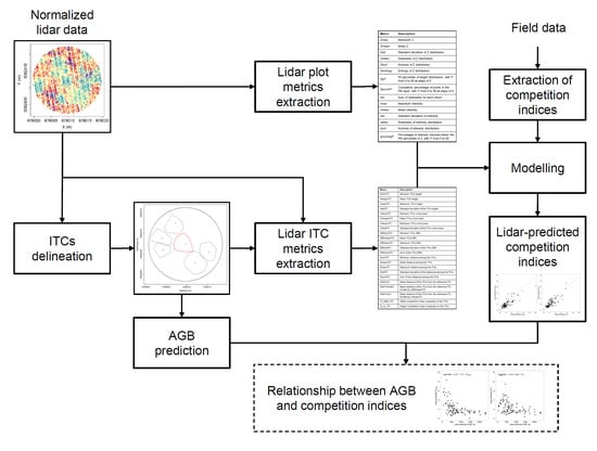
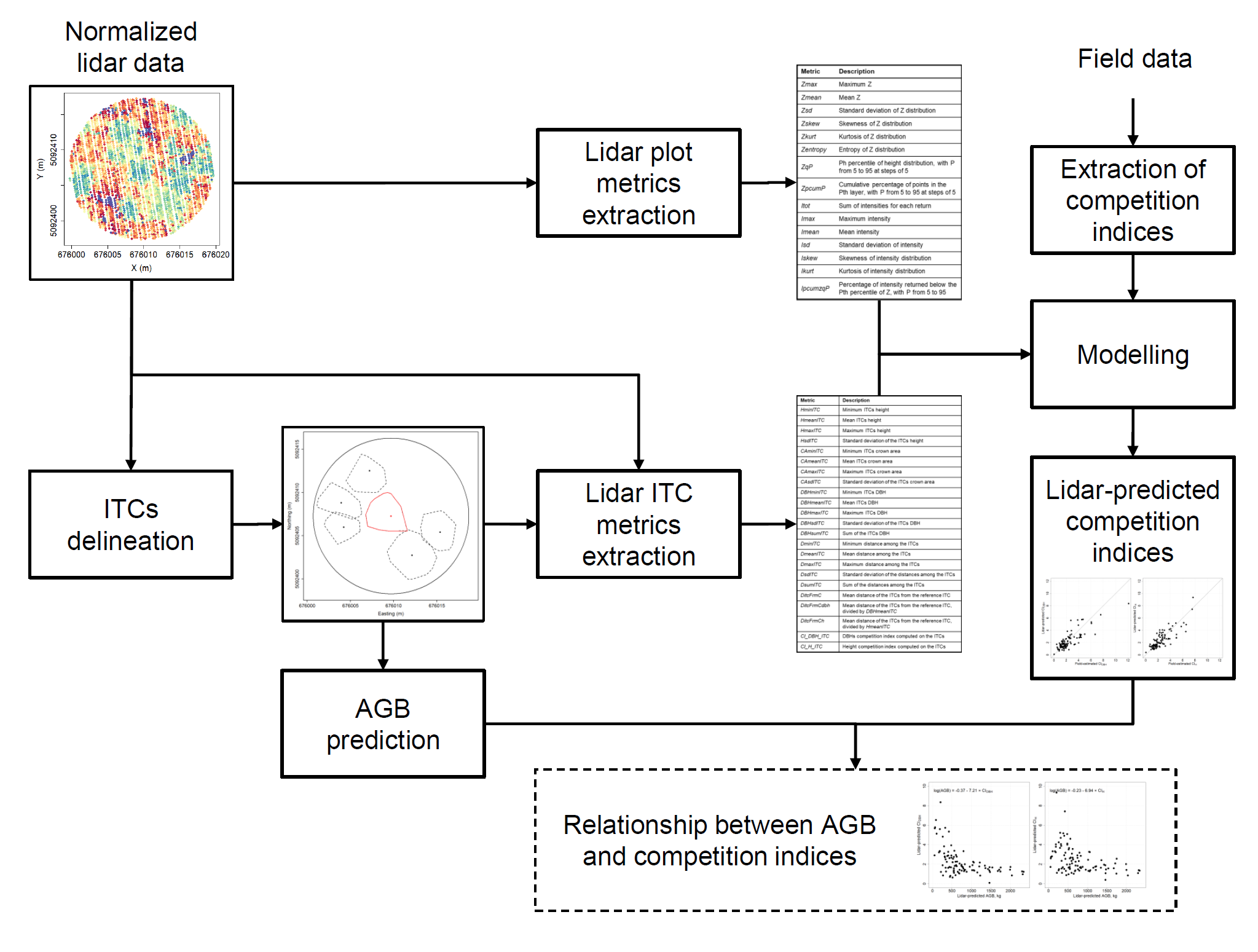
2. Materials and Methods

The workflow in Figure 1 shows the analyses carried out in this work. In the following subsections, we present the dataset analyzed in this study and each step of the workflow.

2.1. Data Set Description

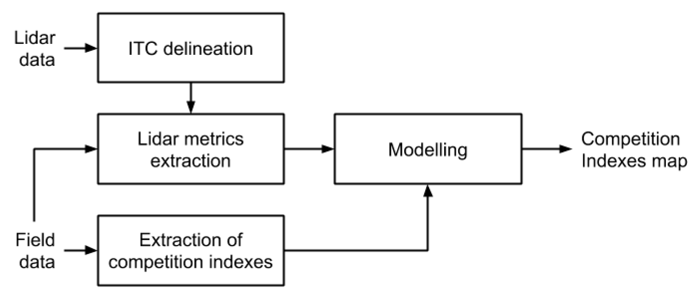
2.1.1. Study Area

This study was conducted in the Autonomous Province of Trento (Italy), in the municipality of Lavarone (45°57′30.09”N, 11°16′25.17′’E). The study area of approximately 4 km² (Figure 2) presents an altitude between 1200 and 1600 m above sea level, and it is composed of an uneven-aged forest with patches of mixed-species and pure-forest stands. The average number of trees per hectare is 839.4. In particular, dominant tree species are Norway spruce (Picea abies (L.) H. Karst.), about 47% of the total stem volume, and silver fir (Abies alba Mill.), about 36% of the total stem volume. Other tree species are present in the study area, although with a low percentage of the total stem volume: European beech (Fagus sylvatica L.) with about 13%, and European larch (Larix decidua Mill.) and Scots pine (Pinus sylvestris L.) with an overall percentage of about 4%.

2.1.2. Lidar Data

Lidar data were acquired in 2015 by an Optech ALTM 3100EA sensor with a maximum scan angle of 21 degrees. The mean point density was 21.5 points per square meter for the first return. Up to four returns per pulse were measured. A digital terrain model (DTM) was generated from the lidar points by the vendor using the TerraScan software with a grid size of 0.5 m. The lidar point cloud was normalized to create a canopy height model (CHM) by subtracting the DTM from the z values of the lidar pulses. This operation was carried out using the software lasground of the package LAStools (https://rapidlasso.com/). The intensity value of each lidar point was range calibrated using the following equation:

$$I_C=I\ast {\left(\frac{R}{Rs}\right)}^{\alpha },$$

(1)

where $I_C$ is the calibrated intensity, $I$ is the raw intensity, $R$ is the sensor-to-target range, and $Rs$ is the reference range or average flying height. An exponential factor, $\alpha$, of 2.5 was considered since the environmental factors can be considered stable and the same acquisition parameters and instruments were maintained during the survey [45].

2.1.3. Field Data

Inside the study area, 49 circular plots of a 15-m radius were placed (see Figure 2). In summer 2016, within each plot, diameter at breast height (DBH), species, and positions were measured for all the trees with DBH ≥ 7 cm. Height was measured only for certain trees while for the others, it was predicted using height–DBH models defined on the basis of the measured trees. Above-ground biomass was obtained for all trees using local stem volume equations [46,47] multiplied by a conversion factor [48]. In

Table 1. Summary of the field data collected in the 49 field plots. Data refer to the mean, maximum, and minimum values.

	All Trees	Norway Spruce	Silver Fir
Height (m)	16.9 (40.1, 2.1)	20.5 (40.1, 3.1)	18.1 (40.0, 3.2)
DBH (cm)	22.3 (81.0, 7.0)	28.6 (79.5, 7.0)	25.4 (81.0, 7.0)
AGB (kg)	284.7 (3468.5, 1.2)	453.5 (3215.0, 1.6)	353.6 (2917.7, 1.6)
$C{I}_H$	5.1 (19.3, 0.04)	5.0 (18.3, 0.7)	4.2 (19.3, 0.04)
$C{I}_{DBH}$	5.7 (22.8, 0.02)	5.1 (17.5, 0.5)	4.3 (15.8, 0.02)

, a summary of the collected field data and plot characteristics is presented.

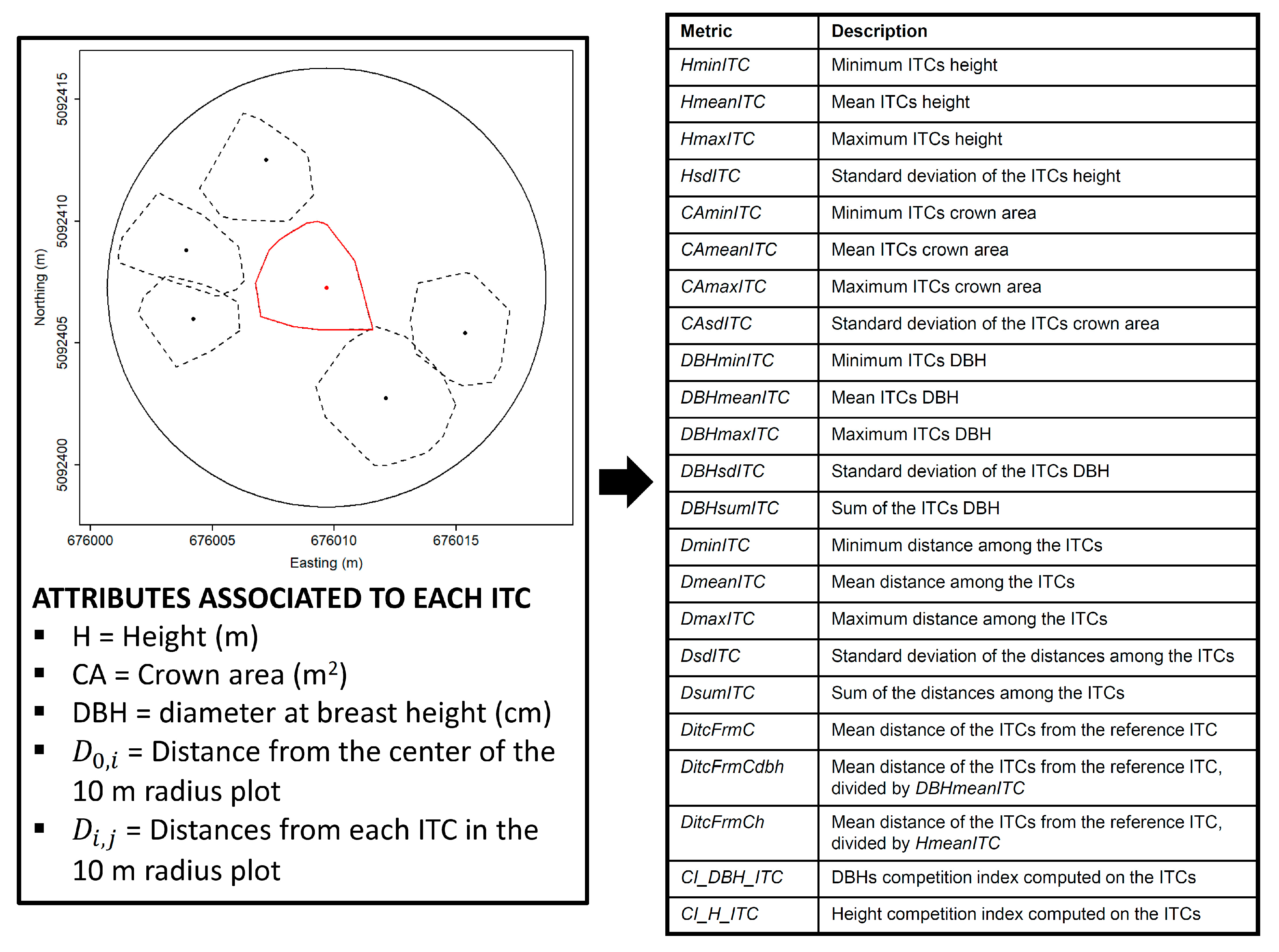
2.2. Extraction of Competition Indices

Competition dynamics were analyzed using distance-dependent individual competition indices (CIs). These indices provide spatial information of the competitive status of an individual tree [49]. In this study, we used the indices proposed by Hegyi [50] in order to represent different combinations of tree characteristics (i.e., DBH and height).

The first step to calculate individual-based competition indices for a tree (called the subject tree) is the identification of the trees actively competing with it. A search radius around the subject tree needs to be defined: The radius influences the number of competitors to consider and thus the indices. A too small or too large radius may lead to underestimates or overestimates of the competitive effects between the subject tree and its real competitors [49]. In the literature, different methods to define the neighborhood area are presented. In our case, to evaluate the level of competition for each tree, we considered only the competitors located within a certain radius from the subject tree. Previous studies showed that a search radius of 10 m is sufficiently wide to capture all the competitive effects of neighboring trees [51,52]. In particular Szwagrzyk et al. [53] used a radius of 10 m in an area with similar structural parameters to the area in this study. Thus, we decided to use such a value. Moreover, to avoid edge effects, the competition indices were calculated only for trees positioned less than 10 m from any of the plot borders.

Two competition indices were considered in this study, one related to stem DBH and one to tree height. The two indices were calculated using the following formulas [50]:

$$C{I}_{DBH}^i={{\displaystyle \sum }}_{j=1}^n\left(\frac{\frac{DB{H}_j}{DB{H}_i}}{dis{t}_{ij}+1}\right),$$

(2)

$$C{I}_H^i={{\displaystyle \sum }}_{j=1}^n\left(\frac{\frac{H_j}{H_i}}{dis{t}_{ij}+1}\right),$$

(3)

where $C{I}_{DBH}^i$ and $C{I}_H^i$ are the DBH and height competition indices for the subject tree, i; $DB{H}_i$ is the diameter at breast height of the subject tree, i; $DB{H}_j$ is the diameter at breast height of the competitor tree, j; $H_i$ is the height of the subject tree, i; $H_j$ is the height of the competitor tree, j; $dis{t}_{ij}$ is the distance between the subject tree, i, and the competitor tree, j; and n is the number of competitors in the neighborhood zone.

Because the most abundant species in our study area are silver fir and Norway spruce, we considered only these species as subject trees, while all trees were competitors.

2.3. ITCs Delineation

The delineation of the ITCs was carried out on the lidar data using the delineation algorithm of the R package itcSegment [54]. In particular, we used the function itcLiDAR. A detailed description of the method adopted can be found in [55]. This approach takes as input the canopy height model (CHM) on which local maxima (i.e., treetops) are located, and around them the crowns of the trees are delineated. The approach included three phases: (1) Smoothing of the canopy height model for which a Gaussian low-pass filter is applied to the rasterized CHM to smooth the surface and to reduce the number of potential local maxima; (2) local maxima extraction: A circular moving window of variable size is applied to the smoothed CHM to find a set of potential treetops (local maxima). A pixel of the CHM is identified as a local maximum when its value is greater than the other values contained in the moving window. The window size is defined according to the height of its central pixel and it spans in a range of odd values defined by the user (e.g., 3,5,7,9). If the height of the central pixel is low, a small value of the window size is used and vice versa; and 3) crown region growing: The crown of a tree is identified by the algorithm through the proximity of the pixels to that particular local maximum. A pixel is considered to belong to a specific region when its vertical distance is less than a percentage of a default difference given by the height of the local maximum. This process is repeated until no pixel is added to a region. Once the region is fully grown, a 2D convex hull is applied, resulting in polygons that represent individual trees (ITCs). The algorithm assigns to each delineated ITC a value of height (i.e., the value of the maximum elevation value of the lidar points inside the ITC) and a value of the crown area derived from the convex hull. The input parameters of the function itcLiDAR used in this study were: Resolution 0.5, MinSearchFilSize 3, MaxSearchFilSize 9, TRESHSeed 0.55, TRESHCrown 0.6, minDIST 5, maxDIST 40, HeightThreshold 2, and cw 1. For each ITC, DBH and AGB were predicted using the equations of Jucker et al. [56] implemented in the R package itcSegment considering the temperate coniferous forest as the biome.

To generate the ITCs dataset to use in the modelling part, a matching process between delineated ITCs and reference ground observations was done. The matching procedure followed two steps: (1) Candidate search: all ground reference trees falling inside an ITC were considered as matching candidates; (2) candidate vote: selected candidates were ranked by their difference in height with the delineated ITCs and their Euclidean distance to the treetop. A distance metric, D, was estimated by considering both parameters to select the best candidate as follows:

$$D=\sqrt{{\left(x_{\mathrm{CAN}}-x_{\mathrm{ITC}}\right)}^2+{\left(y_{\mathrm{CAN}}-y_{\mathrm{ITC}}\right)}^2+w\ast {\left(h_{\mathrm{CAN}}-h_{\mathrm{ITC}}\right)}^2},$$

(4)

where x and y denote the locations and h the heights of the field-measured trees and the delineated ITCs, respectively; $w$ is a user-defined weight (set to 0.5 in this study) [57].

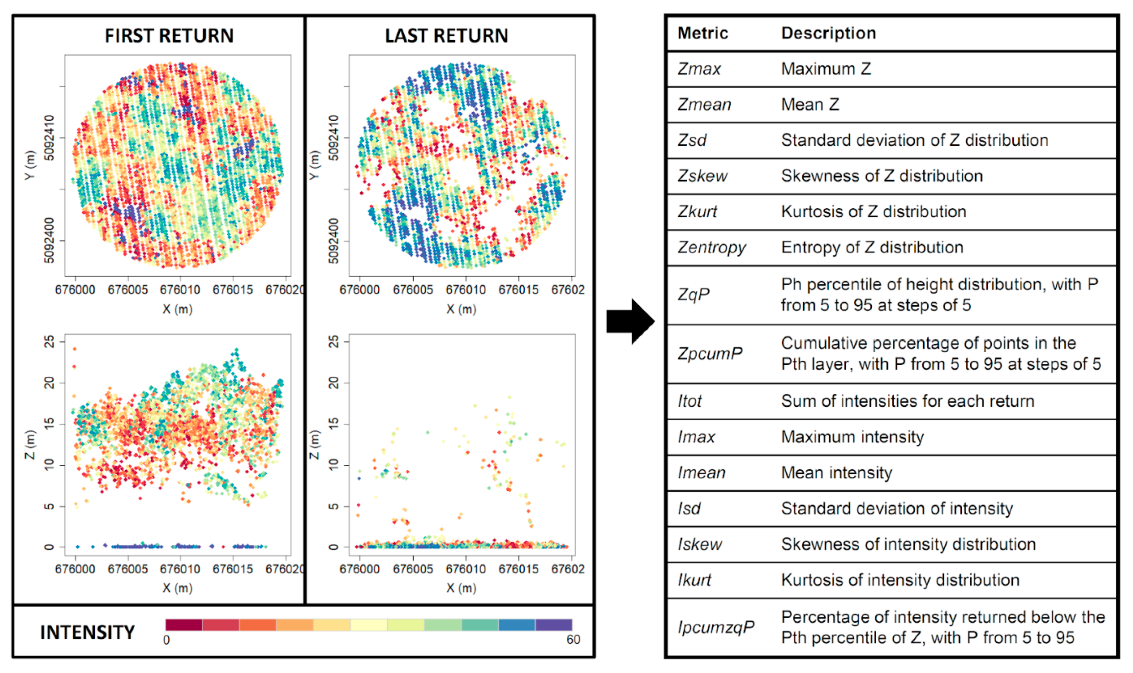
2.4. Lidar Metrics Extraction

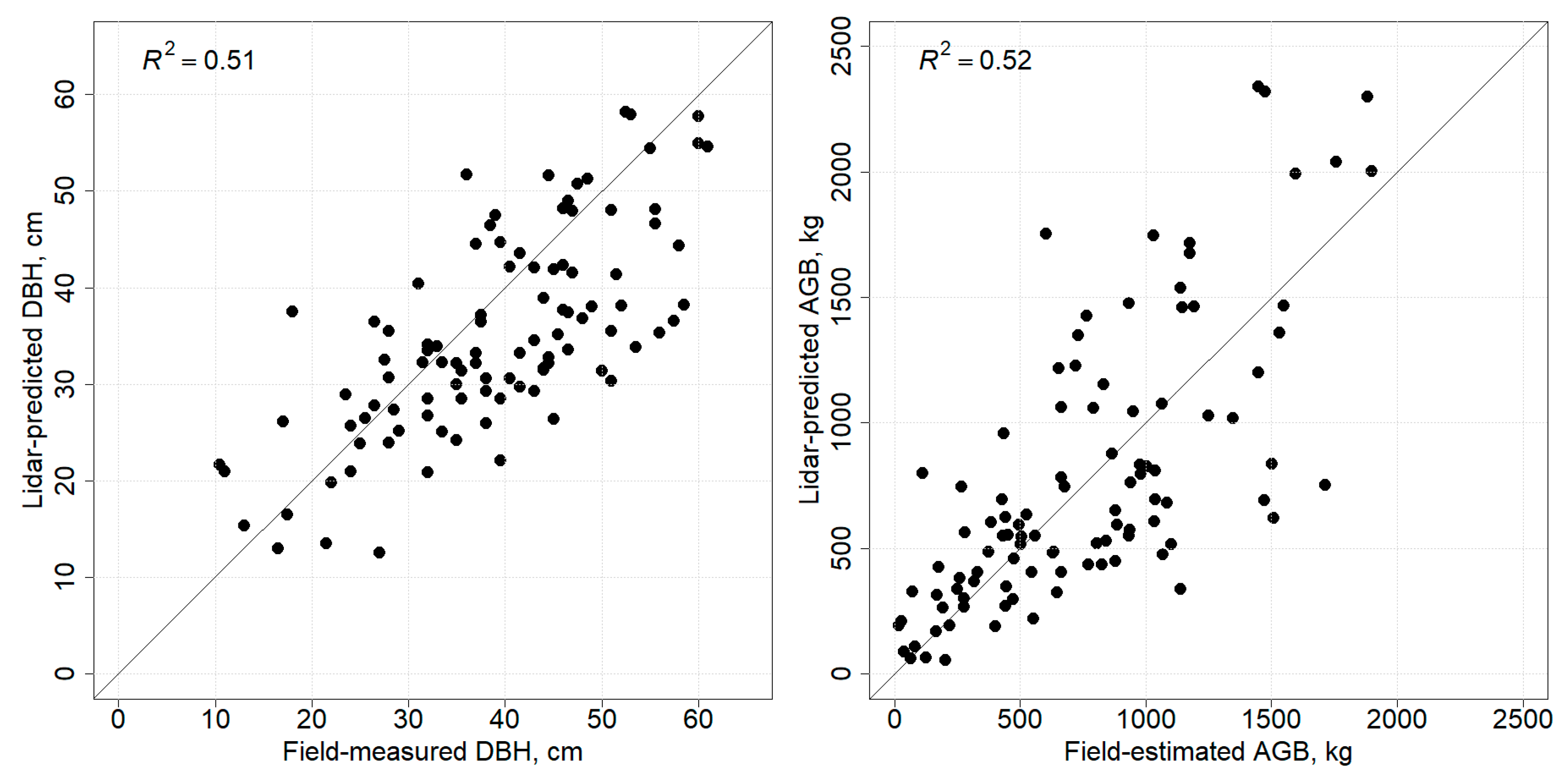
Lidar metrics were extracted for each delineated ITC. As explained before, the competition indices computed on the field tree data refer to the competing trees in a radius of 10 m from the subject tree. Thus, for each ITC, two sets of metrics were defined: (i) plot metrics: 93 elevation and intensity metrics (see Figure 3) extracted from the first and last return of the lidar point cloud data. For each ITC, we considered lidar points located in an area of radius of 10 m from the ITC location. These metrics were extracted from the entire set of points in the 10-m radius from the ITC location, and they did not depend on the ITCs characteristics. Each metric was extracted from the first return points only (_F), and last return points only (_L); and (ii) ITC metrics: 23 metrics computed on the basis of the ITCs located in a radius of 10 m around the considered ITC (see Figure 4). These metrics were computed combining the characteristics (height, crown area, location, DBH) of the ITCs located in a radius of 10 m from the reference ITC.

2.5. Prediction

To evaluate the efficiency of lidar metrics in modelling the competition indices, ordinary least square (OLS) models were built, in which the dependent variables were the competition indices estimated in the field and the independent variables were the lidar metrics. We developed three models for each competition index: One model using all the ITCs matched with the field data, one using only the ones of silver fir, and one using only the ones of Norway spruce. Before building the regression models, the presence of multicollinearity between the independent variables (the lidar metrics) was evaluated with the function findCorrelation of the R package caret [58]. In order to reduce the number of lidar metrics and to remove the ones most correlated among each other, we set the correlation threshold to 0.9. After this, the OLS models were built using the stepAIC function of the R package MASS. A natural logarithmic transformation of the original independent variables (the competition indices) was performed in order to avoid non-normality. The stepAIC function was restricted in order to reduce/avoid overfitting of the models. In particular, the selection was restricted in order to have at least 10 field samples for each metric selected and to have a value of the accuracy indices, $R2R$ (Equation (13)) and $SSR$ (Equation (14)), close to one.

The models were validated using a leave-one-out cross-validation and the accuracy statistics used in [59]. In particular, we considered:

(1) The mean difference (MD) between the predicted and the observed values:

$$\mathrm{MD}={{\displaystyle \sum }}_{i=1}^n\left(pr{e}_i^{CV}-ob{s}_i\right)/n,$$

(5)

where $n$ is the total number of samples, $pr{e}_i^{CV}$ is the predicted value of the sample, i, obtained by cross-validation, and $ob{s}_i$ is the observed value of the sample, i.

(2) The mean absolute difference (MAD):

$$\mathrm{MAD}={{\displaystyle \sum }}_{i=1}^n\left|pr{e}_i^{CV}-ob{s}_i\right|/n.$$

(6)

(3) The root mean squared differences (RMSDs) of the predicted values:

$$\mathrm{RMSD}=\sqrt{S{S}^{CV}/n},$$

(7)

where the $S{S}^{CV}$ is the sum of the squared differences between the observed values and the predicted values obtained by cross-validation:

$$S{S}^{CV}={{\displaystyle \sum }}_{i=1}^n{\left(pr{e}_i^{CV}-ob{s}_i\right)}^2.$$

(8)

(4) The coefficient of determination obtained from the models’ residuals:

$$R_{fit}^2=1-S{S}^{fit}/S{S}_{tot},$$

(9)

where the $S{S}^{fit}$ is the sum of squares of the model residuals:

$$S{S}^{fit}={{\displaystyle \sum }}_{i=1}^n{\left(pr{e}_i^{fit}-ob{s}_i\right)}^2,$$

(10)

and $S{S}_{tot}$ is the sum of squared differences of each observation from the overall mean:

$$S{S}_{tot}={{\displaystyle \sum }}_{i=1}^n{\left(ob{s}_i-\overline{obs}\right)}^2.$$

(11)

(5) The coefficient of determination obtained from the cross-validation:

$$R_{CV}^2=1-S{S}^{CV}/S{S}_{tot}.$$

(12)

(6) The $R_{}^2$ ratio:

$$R2R=R_{fit}^2/R_{CV}^2,$$

(13)

and (7) the sum of squares ratio:

$$SSR=\sqrt{S{S}^{CV}}/\sqrt{S{S}^{fit}}.$$

(14)

Each one of these statistics measures a different aspect of the prediction accuracy: MD measures the prediction bias, MAD and RMSD the prediction precision, $R_{CV}^2$ the agreement, and $R2R$ and $SSR$ the overfitting. Regarding these last statistics, a desirable value for $R2R$ and $SSR$ in order to avoid overfitting is below 1.1 [59].

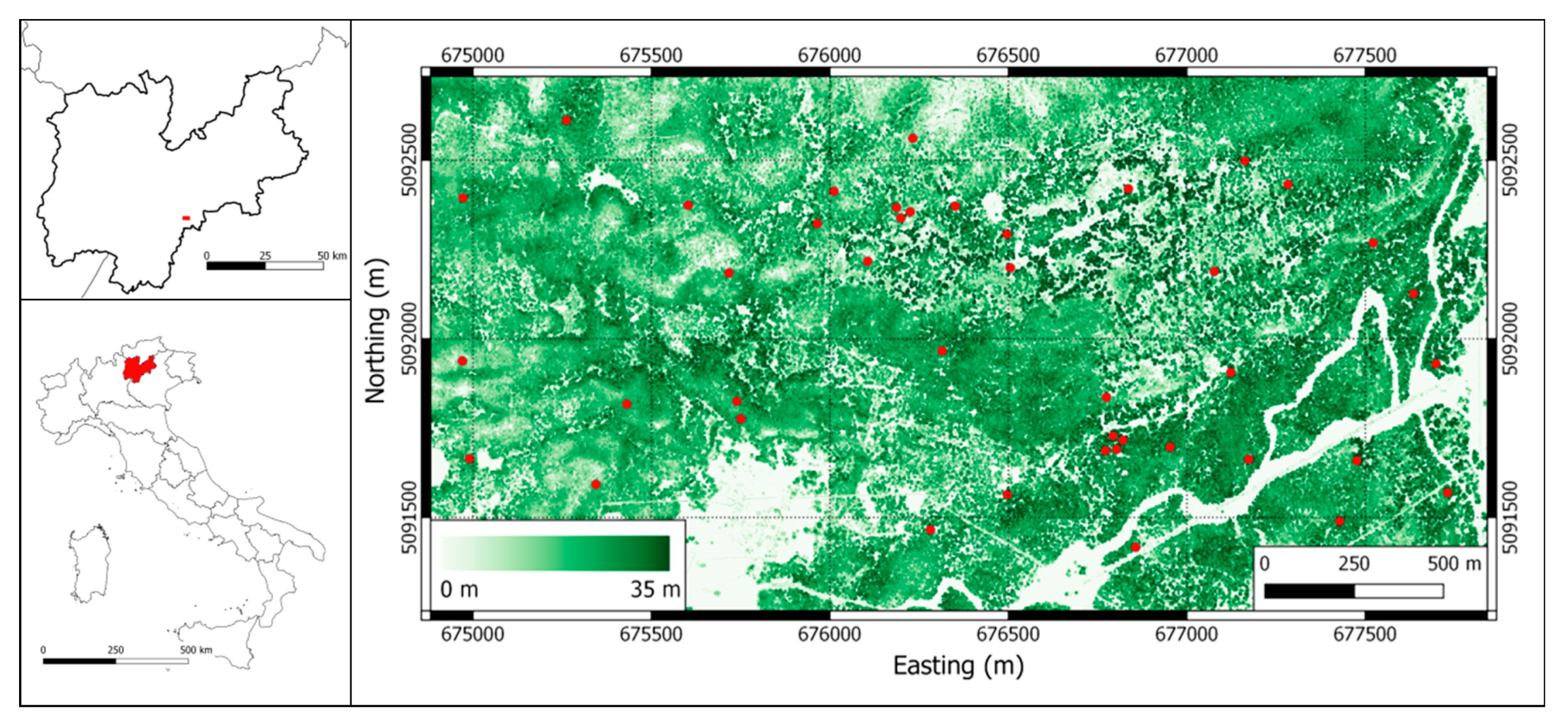
2.6. Relationship between AGB and Competition Indices

The relationship between competition and AGB was evaluated by developing two linear models between the AGB of the subject trees and the corresponding competition indices. In particular, we built: (i) an OLS model linking the logarithm of the individual trees AGB estimated in the field with the competition indices estimated in the field, and (ii) an OLS model linking the logarithm of the individual trees AGB predicted using lidar with the competition indices predicted using lidar. The logarithm was used in order to avoid non-linearity. The coefficient of determination was used to evaluate the relationships.

3. Results

3.1. ITC Crown Delineation

Out of 464 trees used as subject trees to calculate the competition indices, only 115 matched with a delineated ITC. The detection rate was not very high at only 24.7%, but it is worth noting that, as we wanted to use these data to build up a reliable model, we excluded all the matched trees for which the field height and lidar height differed by more than 2 m. Among the 115 matched trees, 100 belonged to Norway spruce (34 ITCs) and silver fir (66 ITCs), and in the following analyses, only these ones were considered. In Figure 5, a scatterplot of the field-measured/estimated versus lidar-predicted values of DBH and AGB is reported along with the R².

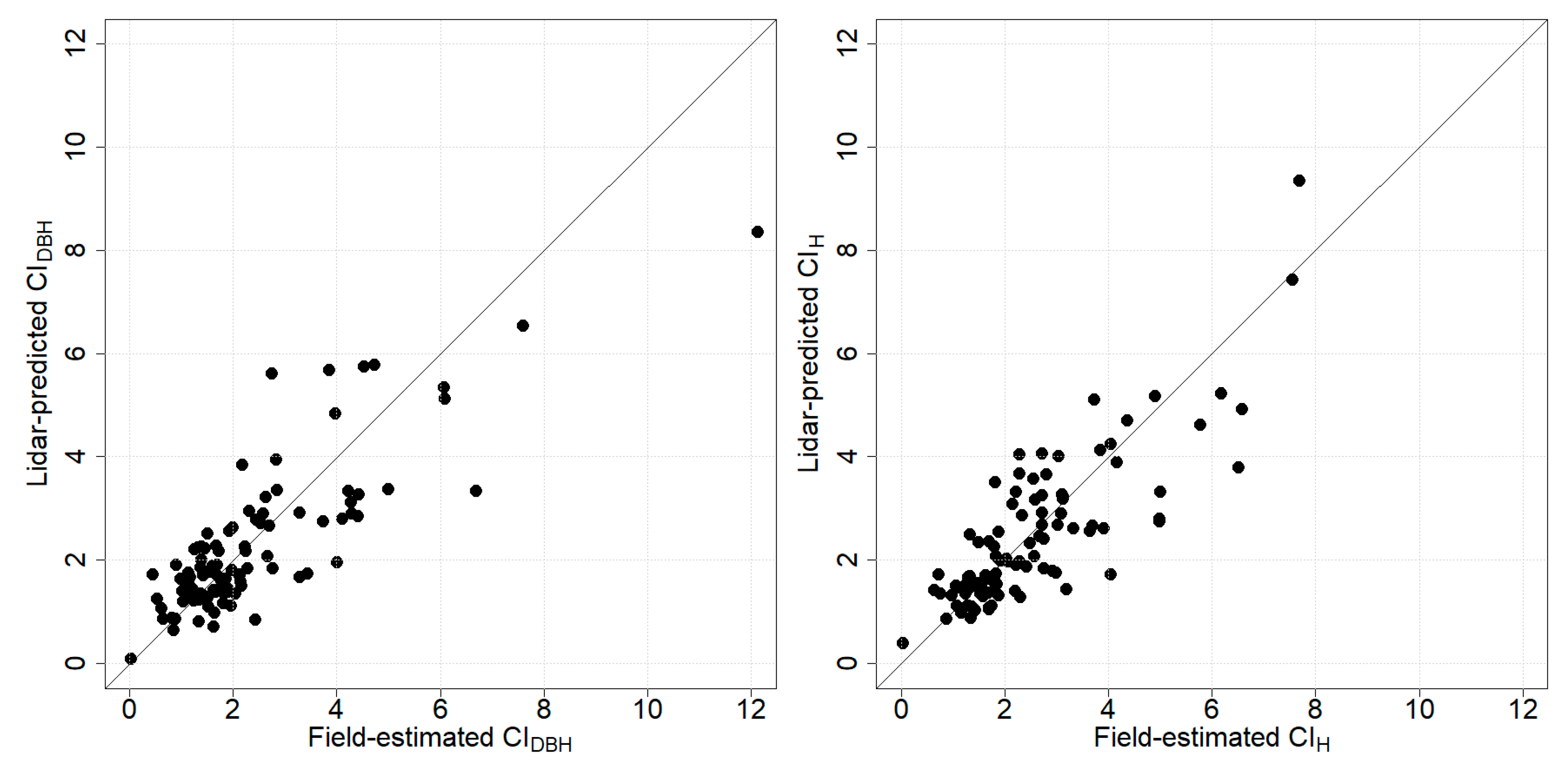
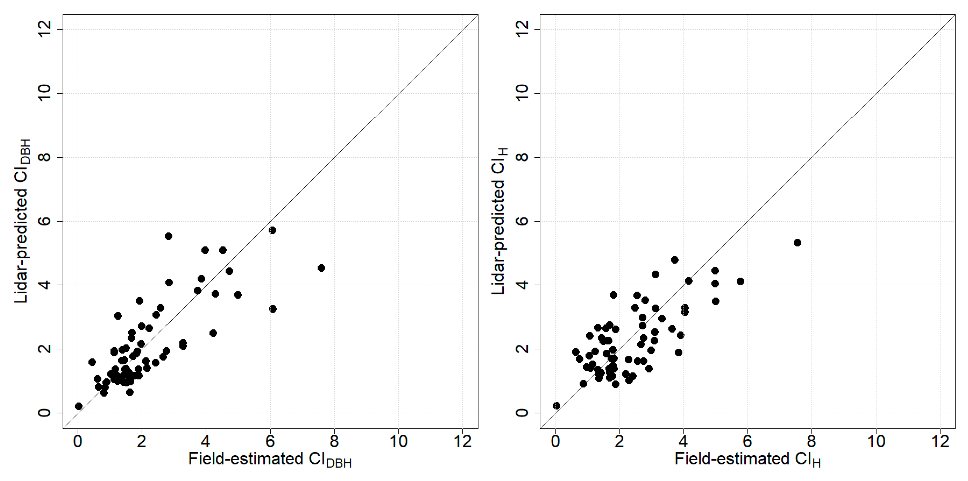
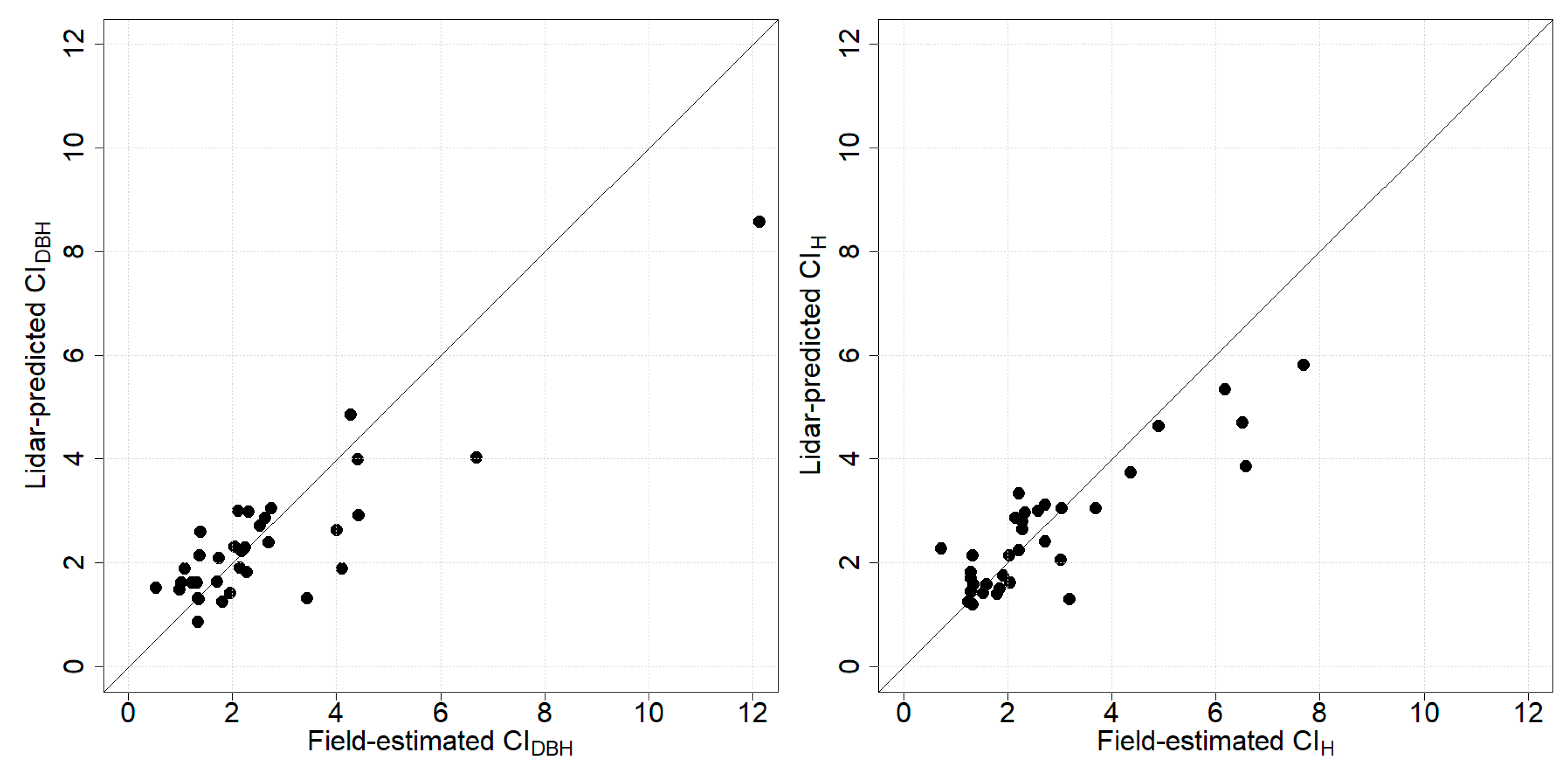
3.2. Prediction of Competition Indices

Regarding the models comprising both species, the $C{I}_{DBH}^{}$ model (

Table 2. OLS model for the prediction of $C{I}_{DBH}^{}$.

Lidar Metric	Estimate	Std. Error	p	Significance
(Intercept)	−2.77	0.52	0.00	***
CI_H_ITC	1.82	0.21	0.00	***
Zpcum1_F	−0.02	0.00	0.00	***
Iskew_L	−0.28	0.11	0.01	*
DBHsumITC	−0.01	0.00	0.00	***
DsdITC	0.30	0.08	0.00	***
CAmeanITC	0.03	0.01	0.00	***

Significance levels: *** = p < 0.001; ** = p < 0.01; * = p < 0.05.

) was made up of two plot metrics and four ITC metrics. Among the plot metrics, one was an elevation metric (Zpcum1_F) and one was an intensity metric (Iskew_L). The $C{I}_H^{}$ model (

Table 3. OLS model for the prediction of $C{I}_H^{}$.

Lidar Metric	Estimate	Std. Error	p	Significance
(Intercept)	2.13	0.58	0.00	***
CI_H_ITC	0.59	0.11	0.00	***
Iskew_F	0.37	0.11	0.00	**
Zpcum2_F	−0.02	0.00	0.00	***
Isd_L	−0.15	0.04	0.00	***
Zq95_L	−0.03	0.01	0.00	**

Significance levels: *** = p < 0.001; ** = p < 0.01; * = p < 0.05.

) was made up of four plot metrics and one ITC metric. Among the plot metrics, two were elevation metrics (Z) and two were intensity metrics (I). Regarding the species specific models, for the silver fir (

Table 4. OLS models for the prediction of the competition indices for silver fir.

$\mathit{C}{\mathit{I}}_{\mathit{D}\mathit{B}\mathit{H}}^{}$			$\mathit{C}{\mathit{I}}_{\mathit{H}}^{}$
Lidar metric	Estimate	Significance	Lidar metric	Estimate	Significance
(Intercept)	−1.07	***	(Intercept)	−1.25	**
CI_H_ITC	1.42	***	CI_DBH_ITC	0.59	***
Zpcum2_F	−0.03	***	DsdITC	0.43	***
Zq20_F	−0.05	***	Zq95_L	−0.05	***

Significance levels: *** = p < 0.001; ** = p < 0.01; * = p < 0.05.

), the $C{I}_{DBH}^{}$ model was made up of two elevation plot metrics and one ITC metric, while the $C{I}_H^{}$ model was made up of one elevation plot metric and two ITC metrics. Contrastingly, the models for Norway spruce (

Table 5. OLS models for the prediction of the competition indices for Norway spruce.

$\mathit{C}{\mathit{I}}_{\mathit{D}\mathit{B}\mathit{H}}^{}$			$\mathit{C}{\mathit{I}}_{\mathit{H}}^{}$
Lidar metric	Estimate	Significance	Lidar metric	Estimate	Significance
(Intercept)	17.39	**	(Intercept)	3.71	***
Ipcumzq90_F	−0.13	*	Imean_F	−0.10	***
Imean_F	−0.09	**	Isd_L	−0.19	***
Ipcumzq50_L	−0.05	**	Zpcum2_L	0.02	*

Significance levels: *** = p < 0.001; ** = p < 0.01; * = p < 0.05.

) were made up by plot metrics only: three intensity metrics for the $C{I}_{DBH}^{}$ model and one elevation metric and two intensity metrics for the $C{I}_H^{}$ model.

Among the ITC metrics, five of them were used in the models: CI_H_ITC, CI_DBH_ITC, DBHsumITC, CAmeanITC, and DsdITC. CI_H_ITC is the height competition index (Equation (3)) computed using only the detected ITCs in the 10-m radius from the subject tree and the lidar-predicted heights; CI_DBH_ITC is the DBH competition index (Equation (2)) computed using only the detected ITCs in the 10-m radius from the subject tree and the lidar-predicted DBH; DBHsumITC is the sum of the predicted DBH values of the delineated ITCs in the 10-m radius around the subject tree; CAmeanITC is the mean value of the crown areas of the delineated ITCs in the 10-m radius around the subject tree; and DsdITC is the standard deviation of the distances among the delineated ITCs in the 10-m radius around the subject tree. Among the elevation plot metrics, two percentile metrics were used (Zq20_F, and Zq95_L) and three cumulative percentage of points metrics (Zpcum1_F, Zpcum2_F, and Zpcum2_L). Six intensity plot metrics were used: Iskew_L, Iskew_F, Isd_L, Imean_F, Ipcumzq50_L, and Ipcumzq90_F.

The accuracy statistics of the models obtained with the leave-one-out cross-validation are shown in

Table 6. Summary of models’ accuracy statistics. MD: mean difference (Equation (5)). MD: relative MD. MAD: mean absolute difference (Equation (6)). MAD%: relative MAD. RMSD: root mean squared differences (Equation (7)). RMSD%: relative RMSD. $R_{fit}^2$: coefficient of determination obtained from the models’ residuals (Equation (9)). $R_{CV}^2$: coefficient of determination obtained from the cross validation (Equation (12)). R2R: the $R_{}^2$ ratio (Equation (13)). SSR: sum of squares ratio (Equation (14)).

	All Trees		Silver Fir		Norway Spruce
	$\mathit{C}{\mathit{I}}_{\mathit{D}\mathit{B}\mathit{H}}^{}$	$\mathit{C}{\mathit{I}}_{\mathit{H}}^{}$	$\mathit{C}{\mathit{I}}_{\mathit{D}\mathit{B}\mathit{H}}^{}$	$\mathit{C}{\mathit{I}}_{\mathit{H}}^{}$	$\mathit{C}{\mathit{I}}_{\mathit{D}\mathit{B}\mathit{H}}^{}$	$\mathit{C}{\mathit{I}}_{\mathit{H}}^{}$
Number of samples	100	100	66	66	34	34
Metrics selected	6	5	3	3	3	3
MD	−0.11	−0.09	−0.09	−0.11	−0.30	−0.20
MD%	−4.8	−3.4	−4.1	−4.5	−11.4	−7.2
MAD	0.75	0.67	0.70	0.83	0.89	0.71
MAD%	31.9	26.7	32.0	34.3	33.9	25.7
RMSD	1.03	0.92	0.98	0.99	1.37	1.00
RMSD%	43.9	36.3	44.7	41.2	52.0	36.3
$R_{fit}^2$	0.68	0.66	0.60	0.53	0.72	0.73
$R_{CV}^2$	0.64	0.62	0.54	0.44	0.57	0.66
R2R	1.08	1.07	1.11	1.19	1.27	1.10
SSR	1.07	1.07	1.07	1.08	1.25	1.11

. As can be seen, the behaviors are quite different for each model. Regarding the generic models, the model for the prediction of $C{I}_H^{}$ obtained slightly better results compared to the one for the prediction of $C{I}_{DBH}^{}$: All the statistics except for the $R_{fit}^2$ and $R_{CV}^2$ obtained better values. Among the species-specific models, the ones for the silver fir competition indices had better performances compared to the ones of Norway spruce. All models experienced quite high values of MAD% (over 25%) and RMSD% (over 36%), and all had a negative bias (negative value of MD). Regarding the overfitting statistics (R2R and SSR), it can be seen that only the generic models have values below 1.1 while for the other models, these values can be higher even if (except for the one for $C{I}_{DBH}^{}$ of Norway spruce) the values are just slightly above 1.1. Figure 6, Figure 7 and Figure 8 show the scatterplots between the competition indices predicted by the lidar models and those calculated from the data in the field.

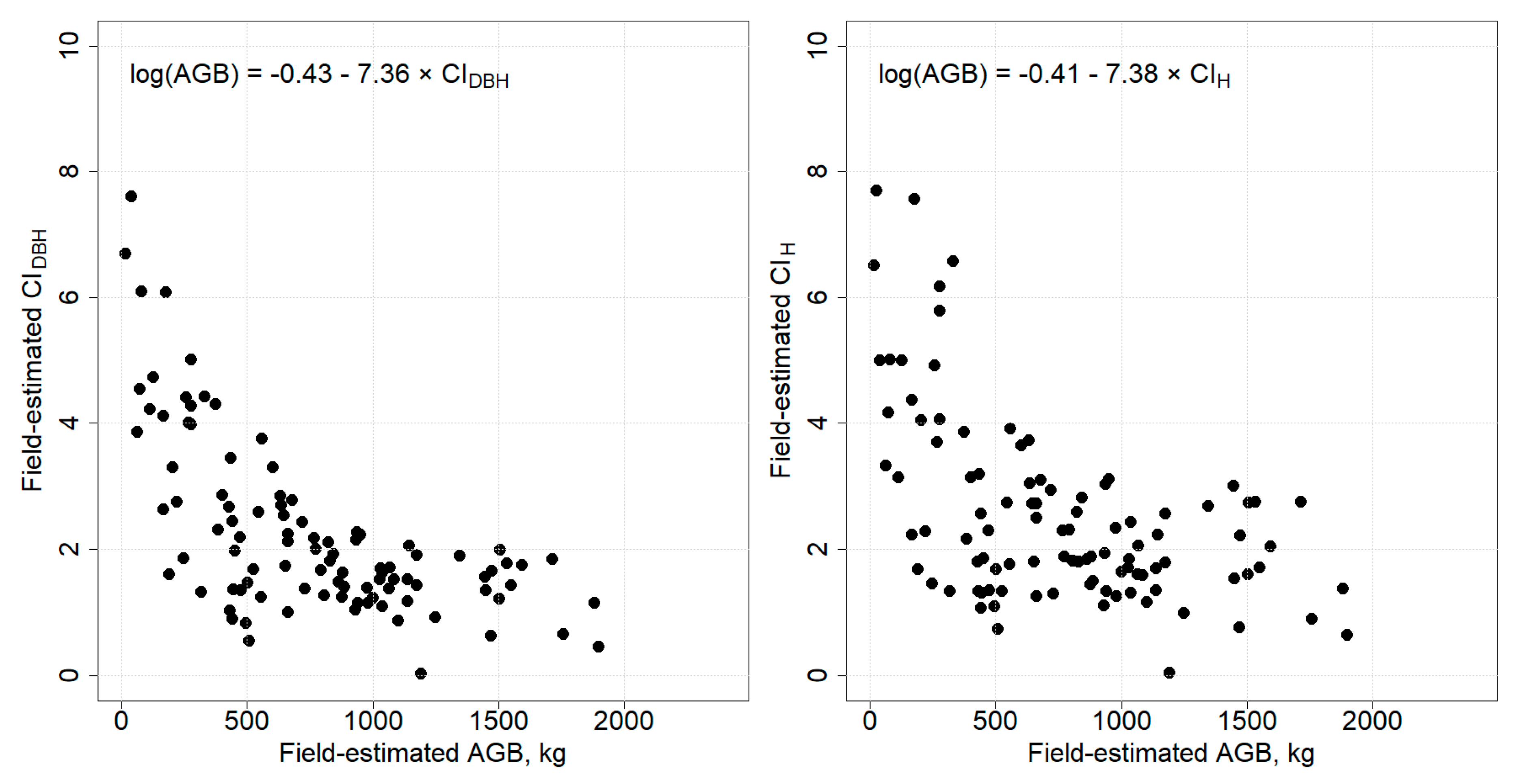
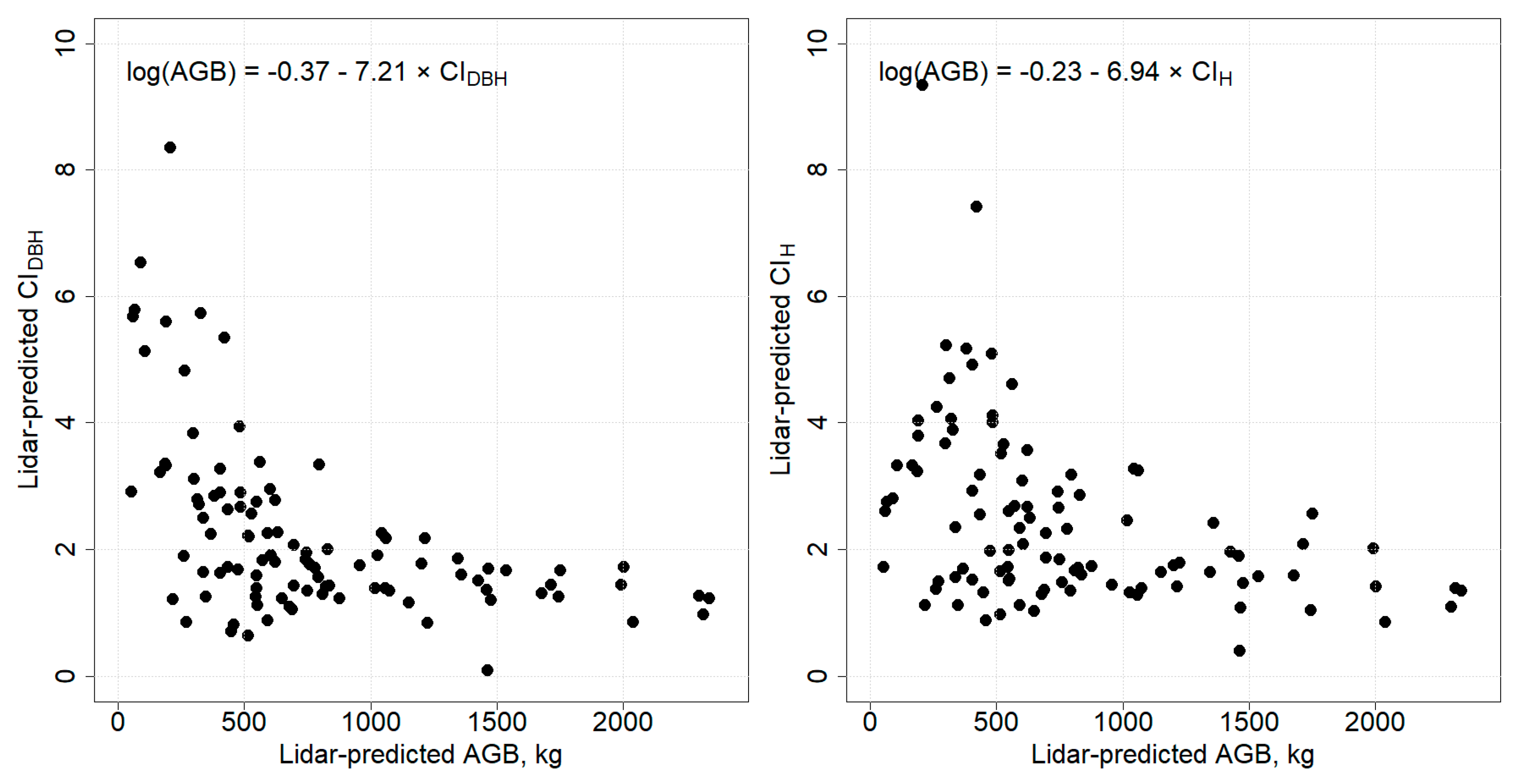
3.3. Relationship between Competition Indices and AGB

In Figure 9 scatterplots of the field-estimated AGB and field-estimated competition indices are shown. This figure shows that high levels of competition resulted in low biomass values while when the competition was below a certain value, it did not influence the biomass. In the figures, the linear models relating the AGB and competition indices are also shown. The model relating log(AGB) to $C{I}_{DBH}^{}$ showed an R² of 0.65 while the one relating log(AGB) to $C{I}_H^{}$ was 0.44. The same trend was found using the lidar-predicted AGB and competition indices (Figure 10), but with lower values of correlation (R² of 0.43 and 0.16, respectively).

4. Discussion

In this study, we demonstrated that it is possible to predict DBH and height competition indices using lidar metrics. We also showed how competition affects the AGB of individual trees. The results showed that no real improvement is gained in using a species-specific model with respect to a general model. It is worth noting that for the species-specific models, we had quite a low number of samples (especially for Norway spruce) and this could have influenced the results. In terms of overfitting, all models showed reasonable values of R2R and SSR; in particular, only the model for $C{I}_{DBH}^{}$ of Norway spruce showed values much above 1.1, which was suggested by Lipovetsky [60] as a desirable limit in order to not have overfitting.

Analysis of the five ITC metrics selected indicated that they are all related to the competition indices. Some of them are clearly related, like the $C{I}_{DBH}^{}$ and $C{I}_H^{}$ indices computed using the ITCs (CI_DBH_ITC, and CI_H_ITC), while the others are representative of a part of the competition index equations (DBHsumITC, and CAmeanITC) and of the density of the forest (DsdITC), which is related to competition. Regarding the plot metrics, it was slightly harder to find a direct relation to the competition indices. Metrics based on the distribution of Z are likely related to competition even if not directly. The Zq20_F, Zq95_L, Zpcum1_F, Zpcum2_F, and Zpcum2_L metrics describe the vertical distribution of the lidar points, and the vertical distribution of the points is related to the forest structure and density, which are related to competition. In contrast, the intensity metrics could be related to the species. As an example, Imean_F has a quite different distribution of values for the two species: It has a mean value of 23.47 (standard deviation of 3.63) for silver fir compared to 20.15 (standard deviation of 3.82) for Norway spruce.

The effectiveness of lidar metrics in predicting both AGB and competition indices was also found in the study conducted by Lin et al. [43]. In particular, Lin et al. [43] showed that the height competition index estimated by lidar, especially when combined with other lidar metrics (crown radius and height) of the trees, is capable of effectively estimating above-ground carbon (AGC) at both the stand and tree level. In our case, the competition indices were used to assess the influence that high or low competition values have on biomass. The results showed that high competition values led to a decrease in biomass. Therefore, the competitive pressure of neighboring trees is probably an important factor influencing tree growth and biomass partitioning, especially for small trees. Indeed, according to Litton et al. [61] and Poorter et al. [62], biomass partitioning may vary with soil resource availability and with the ability of plants to withstand competition for light. Furthermore, according to the theory of biomass allocation, high competition may increase or reduce biomass allocation in plants [63,64]. Zhou et al. [33] found that the biomass ratio of roots and stems decreased with increasing intensity of competition from neighboring trees, while biomass at the level of branches and leaves increased.

Few previous studies were found in the literature that combined lidar and competition indices. Among the ones present in the literature, the ones of Lo et al. [42], Lin et al. [43], and Ma et al. [44] are the only ones slightly related to this work. In all these studies, competition indices were computed using ITCs automatically delineated on lidar data, in a similar way to our computation of the lidar metrics CI_DBH_ITC and CI_H_ITC. None of these studies analyzed the accuracy of the prediction of competition indices using lidar metrics or validated the predictions using field data. In contrast to the present study, these studies used lidar-predicted competition indices as metrics to predict trees attributes, such as DBH, volume, and carbon density.

Several studies have shown the relationship between radial growth and height growth of trees [65,66] and that the crown:height ratio may quantify competition among trees [67,68]. Therefore, the diameter and height of a tree are not only closely linked to light capture but also to the effects of water, nutrients, and soil conditions [33]. Moreover, according to the results of Zhou et al. [33], during growth, plants change how they are affected by the competition of neighboring plants, and their competitive effect on other plants. This suggests a close relationship between individual competition and tree growth.

In the workflow proposed in this study, some parameters were fixed in a way that could have influenced the final results. The main one was the search radius used to compute the competition indices. Many studies in the literature focusing just on the computation of indices using field data used a different radius for each area analyzed. This is possible if all the tree crowns are measured on the ground; however, that was not our case. Moreover, as we wanted to relate the indices to the lidar data in order to have the possibility of also predicting competition indices in areas not covered by field data, we needed to have a fixed value of the search radius. We chose 10 m as it was used before in other studies investigating forests with similar characteristics [53]. It is worth noting that we also carried out the same analyses using other values, computed in other ways, but the used radius was quite close to 10 m and the final results were very similar or the same.

The ITCs delineation could also have had an effect on the final results. Indeed, the higher the accuracy of the delineation, the more valuable ITC metrics are, and the more trees can be considered as subject trees in the area. The algorithm selected is a simple method when compared with the many algorithms in the literature [69], and has been used successfully in many other studies on forests with similar characteristics (e.g., [47,55]). It was effective for different forest scenarios in a previous study conducted on various forest sites in the Alps [70].

Despite the high potential of lidar technology for the estimation of vegetation parameters, it must be considered that lidar also has limitations. According to Rosette et al. [71], the ability to estimate vegetation parameters (tree height and DTM) decreases in the presence of high terrain slopes and high canopy coverage. Moreover, in very dense forests, it is only able to identify dominant trees, as in our study. Values of competition indices calculated using metrics derived from lidar can be biased due to the fact that small trees are not detected.

5. Conclusions

Our results showed that lidar metrics have a good capacity to predict competition indices. We developed a system that, after detecting individual tree crowns (ITCs) in the forest, on the basis of lidar metrics extracted in the neighborhood of the detected ITC, predicts two competition indices related to height and diameter at breast height (DBH). From the analyses, it emerged that the use of lidar metrics based on ITCs is important in prediction models. Moreover, we showed that all the information that can be extracted from lidar data should be used, as both plots and ITCs metrics were used in our models. Regarding the relationship between AGB and competition indices, it was observed that the AGB value decreases, increasing competition at both the DBH and height level. These results are probably related to the variation in the availability of soil-level resources and the ability of plants to withstand competition for light. The possibility of predicting competition indices in large areas opens interesting perspectives for forest management practices aimed at regulating species mixture, in particular for forests managed extensively with selective logging, typical of many mountain areas.

References

1. Jucker, T.; Avăcăriței, D.; Bărnoaiea, I.; Duduman, G.; Bouriaud, O.; Coomes, D.A. Climate modulates the effects of tree diversity on forest productivity. J. Ecol. 2016, 104, 388–398. [Google Scholar] [CrossRef]
2. Shi, H.; Zhang, L. Local Analysis of Tree Competition and Growth. For. Sci. 2003, 49, 938–955. [Google Scholar] [CrossRef]
3. Liang, H.; Huang, J.-G.; Ma, Q.; Li, J.; Wang, Z.; Guo, X.; Zhu, H.; Jiang, S.; Zhou, P.; Yu, B.; et al. Contributions of competition and climate on radial growth of Pinus massoniana in subtropics of China. Agric. For. Meteorol. 2019, 274, 7–17. [Google Scholar] [CrossRef]
4. Aakala, T.; Berninger, F.; Starr, M. The roles of competition and climate in tree growth variation in northern boreal old-growth forests. J. Veg. Sci. 2018, 29, 1040–1051. [Google Scholar] [CrossRef]
5. Contreras, M.A.; Affleck, D.; Chung, W. Evaluating tree competition indices as predictors of basal area increment in western Montana forests. For. Ecol. Manag. 2011, 262, 1939–1949. [Google Scholar] [CrossRef]
6. Coomes, D.A.; Allen, R.B. Effects of size, competition and altitude on tree growth. J. Ecol. 2007, 95, 1084–1097. [Google Scholar] [CrossRef]
7. Ford, K.R.; Breckheimer, I.K.; Franklin, J.F.; Freund, J.A.; Kroiss, S.J.; Larson, A.J.; Theobald, E.J.; HilleRisLambers, J. Competition alters tree growth responses to climate at individual and stand scales. Can. J. For. Res. 2017, 47, 53–62. [Google Scholar] [CrossRef]
8. Ledermann, T. Evaluating the performance of semi-distance-independent competition indices in predicting the basal area growth of individual trees. Can. J. For. Res. 2010, 40, 796–805. [Google Scholar] [CrossRef]
9. Radtke, P.J.; Westfall, J.A.; Burkhart, H.E. Conditioning a distance-dependent competition index to indicate the onset of inter-tree competition. For. Ecol. Manag. 2003, 175, 17–30. [Google Scholar] [CrossRef]
10. Larocque, G.R. Examining Different Concepts for the Development of a Distance-Dependent Competition Model for Red Pine Diameter Growth Using Long-Term Stand Data Differing in Initial Stand Density. For. Sci. 2002, 48, 24–34. [Google Scholar] [CrossRef]
11. Kahriman, A.; Şahin, A.; Sönmez, T.; Yavuz, M. A novel approach to selecting a competition index: The effect of competition on individual-tree diameter growth of Calabrian pine. Can. J. For. Res. 2018, 48, 1217–1226. [Google Scholar] [CrossRef]
12. McTague, J.; Weiskittel, A. Individual-Tree Competition Indices and Improved Compatibility with Stand-Level Estimates of Stem Density and Long-Term Production. Forests 2016, 7, 238. [Google Scholar] [CrossRef]
13. Metz, J.; Seidel, D.; Schall, P.; Scheffer, D.; Schulze, E.-D.; Ammer, C. Crown modeling by terrestrial laser scanning as an approach to assess the effect of aboveground intra- and interspecific competition on tree growth. For. Ecol. Manag. 2013, 310, 275–288. [Google Scholar] [CrossRef]
14. Sun, S.; Cao, Q.V.; Cao, T. Evaluation of distance-independent competition indices in predicting tree survival and diameter growth. Can. J. For. Res. 2019, 49, 440–446. [Google Scholar] [CrossRef]
15. Kuehne, C.; Weiskittel, A.R.; Waskiewicz, J. Comparing performance of contrasting distance-independent and distance-dependent competition metrics in predicting individual tree diameter increment and survival within structurally-heterogeneous, mixed-species forests of Northeastern United States. For. Ecol. Manag. 2019, 433, 205–216. [Google Scholar] [CrossRef]
16. Hui, G.; Wang, Y.; Zhang, G.; Zhao, Z.; Bai, C.; Liu, W. A novel approach for assessing the neighborhood competition in two different aged forests. For. Ecol. Manag. 2018, 422, 49–58. [Google Scholar] [CrossRef]
17. Stadt, K.J.; Huston, C.; Coates, K.D.; Feng, Z.; Dale, M.R.T.; Lieffers, V.J. Evaluation of competition and light estimation indices for predicting diameter growth in mature boreal mixed forests. Ann. For. Sci. 2007, 64, 477–490. [Google Scholar] [CrossRef]
18. Biging, G.S.; Dobbertin, M. Evaluation of Competition Indices in Individual Tree Growth Models. For. Sci. 1995, 41, 360–377. [Google Scholar] [CrossRef]
19. Tomé, M.; Burkhart, H. Distance-Dependent Competition Measures for Predicting Growth of Individual Trees. For. Sci. 1989, 35, 816–831. [Google Scholar]
20. Dale, V.H.; Doyle, T.W.; Shugart, H.H. A comparison of tree growth models. Ecol. Model. 1985, 29, 145–169. [Google Scholar] [CrossRef]
21. Thorpe, H.C.; Astrup, R.; Trowbridge, A.; Coates, K.D. Competition and tree crowns: A neighborhood analysis of three boreal tree species. For. Ecol. Manag. 2010, 259, 1586–1596. [Google Scholar] [CrossRef]
22. Lang, A.C.; Härdtle, W.; Bruelheide, H.; Geißler, C.; Nadrowski, K.; Schuldt, A.; Yu, M.; von Oheimb, G. Tree morphology responds to neighbourhood competition and slope in species-rich forests of subtropical China. For. Ecol. Manag. 2010, 260, 1708–1715. [Google Scholar] [CrossRef]
23. Purves, D.W.; Lichstein, J.W.; Pacala, S.W. Crown Plasticity and Competition for Canopy Space: A New Spatially Implicit Model Parameterized for 250 North American Tree Species. PLoS ONE 2007, 2, e870. [Google Scholar] [CrossRef]
24. King, D.A.; Davies, S.J.; Supardi, M.N.N.; Tan, S. Tree growth is related to light interception and wood density in two mixed dipterocarp forests of Malaysia. Funct. Ecol. 2005, 19, 445–453. [Google Scholar] [CrossRef]
25. Wyckoff, P.H.; Clark, J.S. Tree growth prediction using size and exposed crown area. Can. J. For. Res. 2005, 35, 13–20. [Google Scholar] [CrossRef]
26. Lu, H.; Mohren, G.M.J.; den Ouden, J.; Goudiaby, V.; Sterck, F.J. Overyielding of temperate mixed forests occurs in evergreen-deciduous but not in deciduous-deciduous species mixtures over time in the Netherlands. For. Ecol. Manag. 2016, 376, 321–332. [Google Scholar] [CrossRef]
27. Forrester, D.I.; Theiveyanathan, S.; Collopy, J.J.; Marcar, N.E. Enhanced water use efficiency in a mixed Eucalyptus globulus and Acacia mearnsii plantation. For. Ecol. Manag. 2010, 259, 1761–1770. [Google Scholar] [CrossRef]
28. Brassard, B.W.; Chen, H.Y.H.; Cavard, X.; Laganière, J.; Reich, P.B.; Bergeron, Y.; Paré, D.; Yuan, Z. Tree species diversity increases fine root productivity through increased soil volume filling. J. Ecol. 2013, 101, 210–219. [Google Scholar] [CrossRef]
29. Bosela, M.; Tobin, B.; Šebeň, V.; Petráš, R.; Larocque, G.R. Different mixtures of Norway spruce, silver fir, and European beech modify competitive interactions in central European mature mixed forests. Can. J. For. Res. 2015, 45, 1577–1586. [Google Scholar] [CrossRef]
30. Fox, T.R.; Jokela, E.J.; Allen, H.L. The Development of Pine Plantation Silviculture in the Southern United States. J. For. 2007, 105, 337–347. [Google Scholar] [CrossRef]
31. Davidson, R.L. Effect of Root/Leaf Temperature Differentials on Root/Shoot Ratios in Some Pasture Grasses and Clover. Ann. Bot. 1969, 33, 561–569. [Google Scholar] [CrossRef]
32. Sebastià, M.-T. Plant guilds drive biomass response to global warming and water availability in subalpine grassland. J. Appl. Ecol. 2006, 44, 158–167. [Google Scholar] [CrossRef]
33. Zhou, W.; Cheng, X.; Wu, R.; Han, H.; Kang, F.; Zhu, J.; Tian, P. Effect of intraspecific competition on biomass partitioning of Larix principis-rupprechtii. J. Plant Interact. 2018, 13, 1–8. [Google Scholar] [CrossRef] [Green Version]
34. Lin, Y.; Huth, F.; Berger, U.; Grimm, V. The role of belowground competition and plastic biomass allocation in altering plant mass-density relationships. Oikos 2014, 123. [Google Scholar] [CrossRef]
35. Cahill, J.F., Jr.; Casper, B.B. Investigating the relationship between neighbor root biomass and belowground competition: Field evidence for symmetric competition belowground. Oikos 2000, 90, 311–320. [Google Scholar] [CrossRef] [Green Version]
36. Petersen, K.S.; Ares, A.; Terry, T.A.; Harrison, R.B. Vegetation competition effects on aboveground biomass and macronutrients, leaf area, and crown structure in 5-year old Douglas-fir. New For. 2008, 35, 299–311. [Google Scholar] [CrossRef]
37. Badreldin, N.; Sanchez-Azofeifa, A. Estimating Forest Biomass Dynamics by Integrating Multi-Temporal Landsat Satellite Images with Ground and Airborne LiDAR Data in the Coal Valley Mine, Alberta, Canada. Remote Sens. 2015, 7, 2832–2849. [Google Scholar] [CrossRef] [Green Version]
38. Hansen, E.; Gobakken, T.; Bollandsås, O.; Zahabu, E.; Næsset, E. Modeling Aboveground Biomass in Dense Tropical Submontane Rainforest Using Airborne Laser Scanner Data. Remote Sens. 2015, 7, 788–807. [Google Scholar] [CrossRef] [Green Version]
39. Sheridan, R.; Popescu, S.; Gatziolis, D.; Morgan, C.; Ku, N.-W. Modeling Forest Aboveground Biomass and Volume Using Airborne LiDAR Metrics and Forest Inventory and Analysis Data in the Pacific Northwest. Remote Sens. 2014, 7, 229–255. [Google Scholar] [CrossRef]
40. Popescu, S.C.; Wynne, R.H.; Scrivani, J.A. Fusion of Small-Footprint Lidar and Multispectral Data to Estimate Plot-Level Volume and Biomass in Deciduous and Pine Forests in Virginia, USA. For. Sci. 2004, 50, 551–565. [Google Scholar] [CrossRef]
41. Simonson, W.; Ruiz-Benito, P.; Valladares, F.; Coomes, D. Modelling above-ground carbon dynamics using multi-temporal airborne lidar: Insights from a Mediterranean woodland. Biogeosciences 2016, 13, 961–973. [Google Scholar] [CrossRef] [Green Version]
42. Lo, C.-S.; Lin, C. Growth-Competition-Based Stem Diameter and Volume Modeling for Tree-Level Forest Inventory Using Airborne LiDAR Data. IEEE Trans. Geosci. Remote Sens. 2013, 51, 2216–2226. [Google Scholar] [CrossRef]
43. Lin, C.; Thomson, G.; Popescu, S. An IPCC-Compliant Technique for Forest Carbon Stock Assessment Using Airborne LiDAR-Derived Tree Metrics and Competition Index. Remote Sens. 2016, 8, 528. [Google Scholar] [CrossRef] [Green Version]
44. Ma, Q.; Su, Y.; Tao, S.; Guo, Q. Quantifying individual tree growth and tree competition using bi-temporal airborne laser scanning data: A case study in the Sierra Nevada Mountains, California. Int. J. Digit. Earth 2018, 11, 485–503. [Google Scholar] [CrossRef]
45. Yu, X.; Hyyppä, J.; Litkey, P.; Kaartinen, H.; Vastaranta, M.; Holopainen, M. Single-Sensor Solution to Tree Species Classification Using Multispectral Airborne Laser Scanning. Remote Sens. 2017, 9, 108. [Google Scholar] [CrossRef] [Green Version]
46. Scrinzi, G.; Galvagni, D.; Marzullo, L. I Nuovi Modelli Dendrometrici Per la Stima Delle Masse Assestamentali in Provincia di Trento. 2010. Available online: http://sito.entecra.it/portale/public/documenti/sff_modelli_dendrometrici.pdf?lingua=EN (accessed on 15 September 2019).
47. Dalponte, M.; Coomes, D.A. Tree-centric mapping of forest carbon density from airborne laser scanning and hyperspectral data. Methods Ecol. Evol. 2016, 7, 1236–1245. [Google Scholar] [CrossRef] [Green Version]
48. IPCC Guidelines for National Greenhouse Gas Inventories. Agriculture, Forestry and Other Land Use. 2006. Available online: https://www.ipcc-nggip.iges.or.jp/public/2006gl/ (accessed on 15 September 2019).
49. Wang, D.; Tang, S.-C.; Hsieh, H.-C.; Chung, C.-H.; Lin, C.-Y. Distance-dependent competition measures for individual tree growth on a Taiwania plantation in the Liuguei area. Taiwan J. For. Sci. 2012, 27, 215–227. [Google Scholar]
50. Hegyi, F. A simulation model for managing jack-pine stands. In Growth Models for Tree and Stand Simulation; Fries, J.R., Ed.; Royal College of Forestry: Stockholm, Sweden, 1974; pp. 74–76. [Google Scholar]
51. Papaik, M.J.; Canham, C.D. Multi-model analysis of tree competition along environmental gradients in southern New England forests. Ecol. Appl. 2006, 16, 1880–1892. [Google Scholar] [CrossRef]
52. Canham, C.D.; LePage, P.T.; Coates, K.D. A neighborhood analysis of canopy tree competition: Effects of shading versus crowding. Can. J. For. Res. 2004, 34, 778–787. [Google Scholar] [CrossRef]
53. Szwagrzyk, J.; Szewczyk, J.; Maciejewski, Z. Shade-tolerant tree species from temperate forests differ in their competitive abilities: A case study from Roztocze, south-eastern Poland. For. Ecol. Manag. 2012, 282, 28–35. [Google Scholar] [CrossRef]
54. Dalponte, M. Package ‘itcSegment’; 2018; pp. 1–12. Available online: https://cran.r-project.org/web/packages/itcSegment/index.html (accessed on 15 September 2019).
55. Dalponte, M.; Frizzera, L.; Ørka, H.O.; Gobakken, T.; Næsset, E.; Gianelle, D. Predicting stem diameters and aboveground biomass of individual trees using remote sensing data. Ecol. Indic. 2018, 85. [Google Scholar] [CrossRef]
56. Jucker, T.; Caspersen, J.; Chave, J.; Antin, C.; Barbier, N.; Bongers, F.; Dalponte, M.; van Ewijk, K.Y.; Forrester, D.I.; Haeni, M.; et al. Allometric equations for integrating remote sensing imagery into forest monitoring programmes. Glob. Chang. Biol. 2017, 23. [Google Scholar] [CrossRef]
57. Zhao, K.; Suarez, J.C.; Garcia, M.; Hu, T.; Wang, C.; Londo, A. Utility of multitemporal lidar for forest and carbon monitoring: Tree growth, biomass dynamics, and carbon flux. Remote Sens. Environ. 2018, 204, 883–897. [Google Scholar] [CrossRef]
58. Kuhn, M. Building Predictive Models in R Using the caret Package. J. Stat. Softw. 2008, 28. [Google Scholar] [CrossRef] [Green Version]
59. Valbuena, R.; Hernando, A.; Manzanera, J.A.; Görgens, E.B.; Almeida, D.R.A.; Mauro, F.; García-Abril, A.; Coomes, D.A. Enhancing of accuracy assessment for forest above-ground biomass estimates obtained from remote sensing via hypothesis testing and overfitting evaluation. Ecol. Model. 2017, 366, 15–26. [Google Scholar] [CrossRef] [Green Version]
60. Lipovetsky, S. How Good is Best? Multivariate Case of Ehrenberg-Weisberg Analysis of Residual Errors in Competing Regressions. J. Mod. Appl. Stat. Methods 2013, 12, 242–255. [Google Scholar] [CrossRef] [Green Version]
61. Litton, C.M.; Raich, J.W.; Ryan, M.G. Carbon allocation in forest ecosystems. Glob. Chang. Biol. 2007, 13, 2089–2109. [Google Scholar] [CrossRef] [Green Version]
62. Poorter, H.; Niklas, K.J.; Reich, P.B.; Oleksyn, J.; Poot, P.; Mommer, L. Biomass allocation to leaves, stems and roots: Meta-analyses of interspecific variation and environmental control. New Phytol. 2012, 193, 30–50. [Google Scholar] [CrossRef]
63. Temesgen, H.; LeMay, V.; Mitchell, S.J. Tree crown ratio models for multi-species and multi-layered stands of southeastern British Columbia. For. Chron. 2005, 81, 133–141. [Google Scholar] [CrossRef]
64. Toma, B. Prediction equations for estimating tree height, crown diameter, crown height and crown ratio of Parkia biglobosa in the Nigerian guinea savanna. Afr. J. Agric. Res. 2012, 7, 6541–6543. [Google Scholar] [CrossRef] [Green Version]
65. Waring, R.; Thies, W.; Muscato, D. Stem Growth per Unit of Leaf Area: A Measure of Tree Vigor. For. Sci. 1980, 26, 112–117. [Google Scholar]
66. Rodríguez, R.; Espinosa, M.; Hofmann, G.; Marchant, M. Needle mass, fine root and stem wood production in response to silvicultural treatment, tree size and competitive status in radiata pine stands. For. Ecol. Manag. 2003, 186, 287–296. [Google Scholar] [CrossRef]
67. Rottmann, M. Waldbauliche Konsequenzen aus Schneebruchkatastrophen. Schweiz. Z. Forstwes. 1985, 136, 167–184. [Google Scholar]
68. Vospernik, S.; Monserud, R.A.; Sterba, H. Do individual-tree growth models correctly represent height:diameter ratios of Norway spruce and Scots pine? For. Ecol. Manag. 2010, 260, 1735–1753. [Google Scholar] [CrossRef] [Green Version]
69. Zhen, Z.; Quackenbush, L.; Zhang, L. Trends in Automatic Individual Tree Crown Detection and Delineation—Evolution of LiDAR Data. Remote Sens. 2016, 8, 333. [Google Scholar] [CrossRef] [Green Version]
70. Eysn, L.; Hollaus, M.; Lindberg, E.; Berger, F.; Monnet, J.-M.; Dalponte, M.; Kobal, M.; Pellegrini, M.; Lingua, E.; Mongus, D.; et al. A benchmark of lidar-based single tree detection methods using heterogeneous forest data from the Alpine Space. Forests 2015, 6, 1721–1747. [Google Scholar] [CrossRef] [Green Version]
71. Rosette, J.; North, P.R.J.; Rubio-Gil, J.; Cook, B.; Los, S.; Suarez, J.; Sun, G.; Ranson, J.; Blair, J.B. Evaluating Prospects for Improved Forest Parameter Retrieval From Satellite LiDAR Using a Physically-Based Radiative Transfer Model. IEEE J. Sel. Top. Appl. Earth Obs. Remote Sens. 2013, 6, 45–53. [Google Scholar] [CrossRef]
Figure 1. Workflow of the processing steps adopted in this study.
Remotesensing 11 02734 g001
Figure 2. Canopy height model of the study area with plot locations (in red). The coordinate system of the CHM is UTM WGS 84 zone 32N. In the insets on the left, on the bottom, a map of Italy with the location of the Autonomous Province of Trento (in red), and, on the top, the location of the study site (in red) inside the Autonomous Province of Trento.
Remotesensing 11 02734 g002
Figure 3. Example of a point cloud in a radius of 10 m from an ITC. The points are colored according to their intensity value. On the right, a table of the metrics extracted from the first and last returns of the lidar points is shown.
Remotesensing 11 02734 g003
Figure 4. Example of competitors’ ITCs (dashed ITCs) in a radius of 10 m from a subject ITC (red ITC), and list of attributes associated with each ITC from which the ITCs’ metrics were extracted. On the right, a table of the metrics extracted is presented.
Remotesensing 11 02734 g004
Figure 5. Field-measured DBH and field-estimated AGB versus lidar-predicted DBH and AGB for the 100 detected trees used to build the competition models.
Remotesensing 11 02734 g005
Figure 6. Field-estimated competition indices versus lidar-predicted competition indices. On the right, the C I D B H competition index, and on the left, the C I H competition index.
Remotesensing 11 02734 g006
Figure 7. Field-estimated competition indices versus lidar-predicted competition indices for silver fir ITCs. On the right, the C I D B H competition index, and on the left, the C I H competition index.
Remotesensing 11 02734 g007
Figure 8. Field-estimated competition indices versus lidar-predicted competition indices for Norway spruce ITCs. On the right, the C I D B H competition index, and on the left, the C I H competition index.
Remotesensing 11 02734 g008
Figure 9. Field-estimated AGB versus field-estimated competition indices for the 100 ITCs matched with the field data.
Remotesensing 11 02734 g009
Figure 10. Lidar-predicted AGB versus lidar-predicted competition indices for the 100 ITCs matched with the field data.
Remotesensing 11 02734 g010