Validation of ICESat-2 ATLAS Bathymetry and Analysis of ATLAS’s Bathymetric Mapping Performance

 ,
,
Abstract
:
1. Introduction
- Can the ICESat-2 ATLAS reliably measure bathymetry, with appropriate refraction corrections applied?
- If so, how accurate is the ATLAS-derived bathymetry?
- What is ATLAS’s maximum depth mapping capability, as a function of water clarity?
2. Materials and Methods
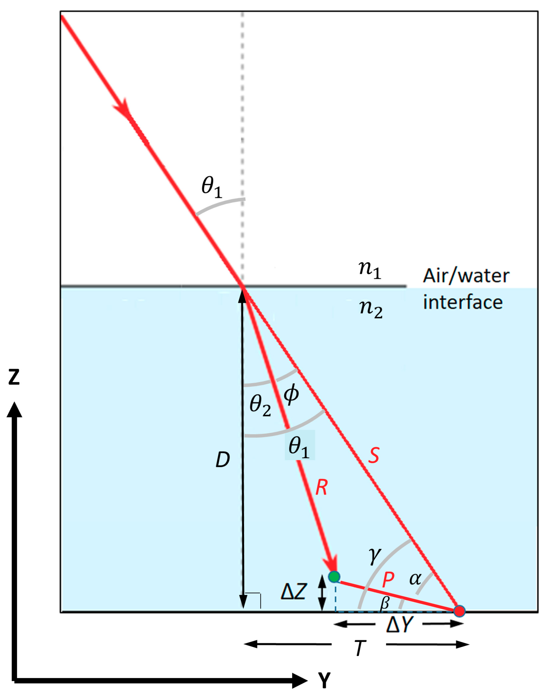
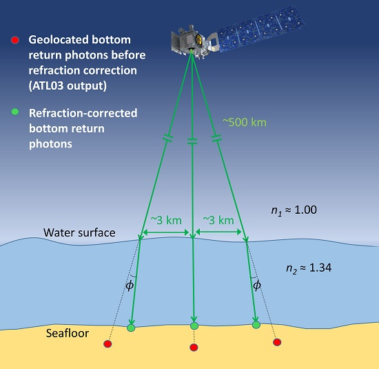
2.1. Refraction Correction
2.2. Study Site
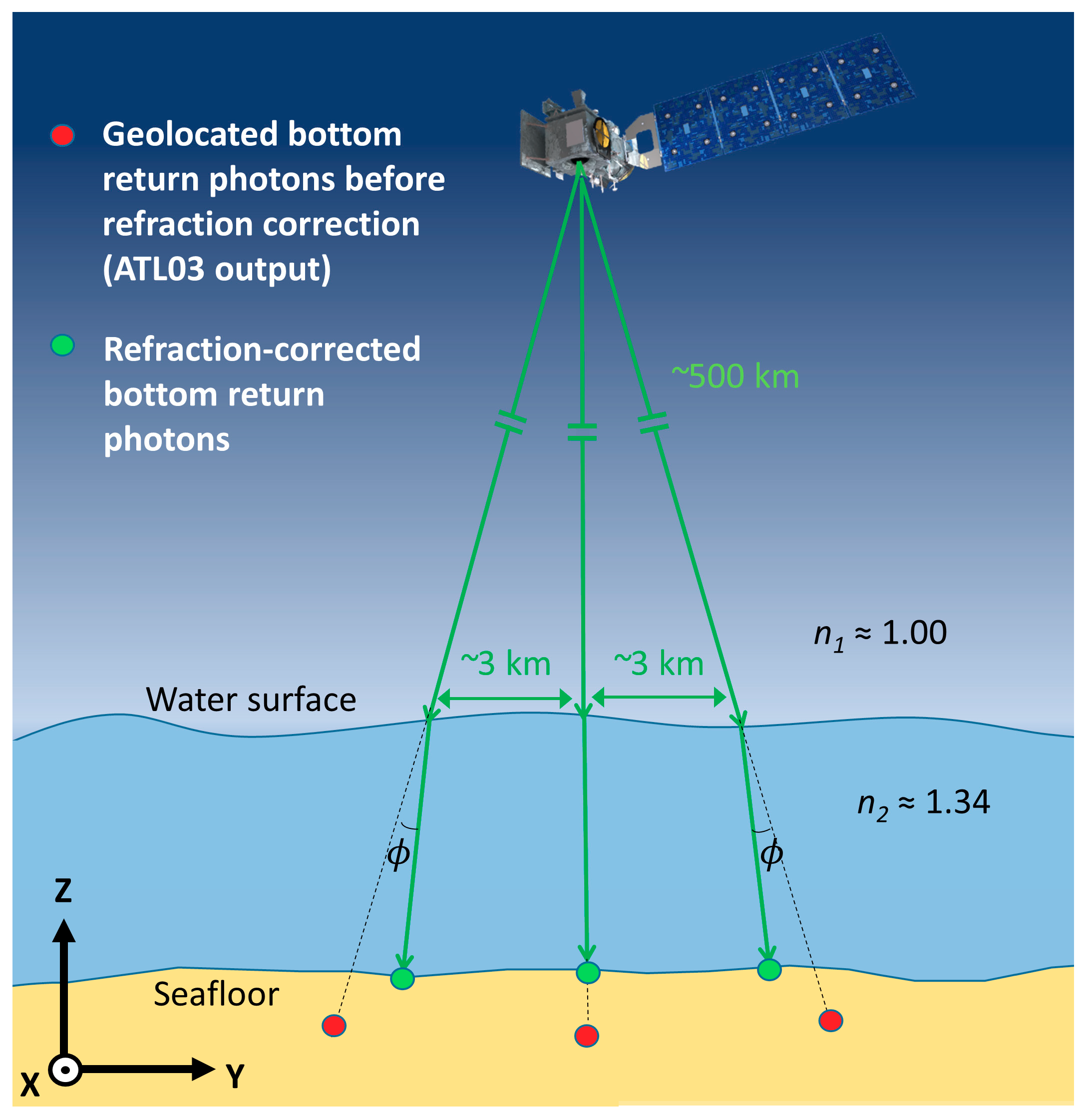
2.3. Reference Data
2.4. ATLAS Data
2.5. Empirical Depth Mapping Performance Determination
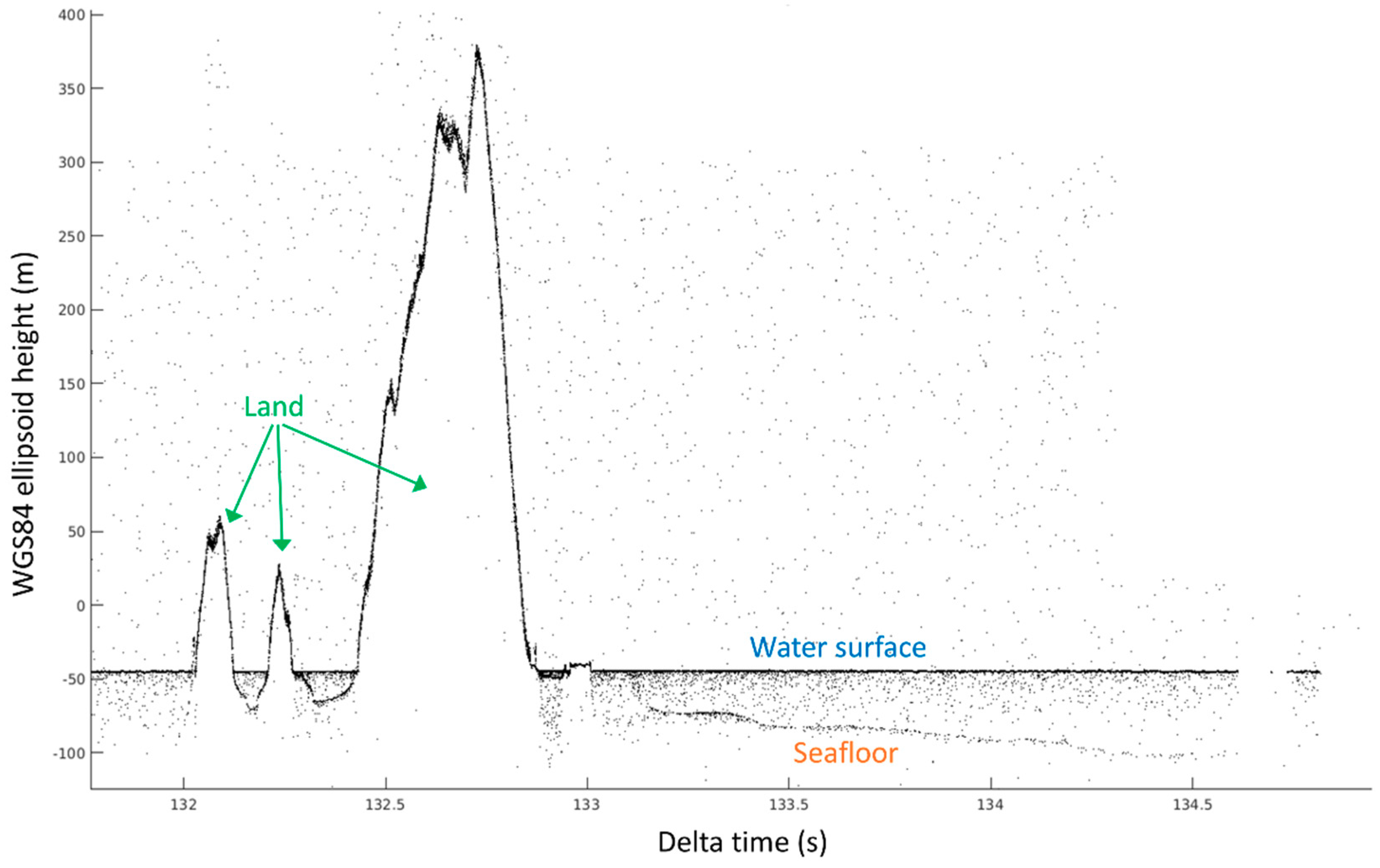
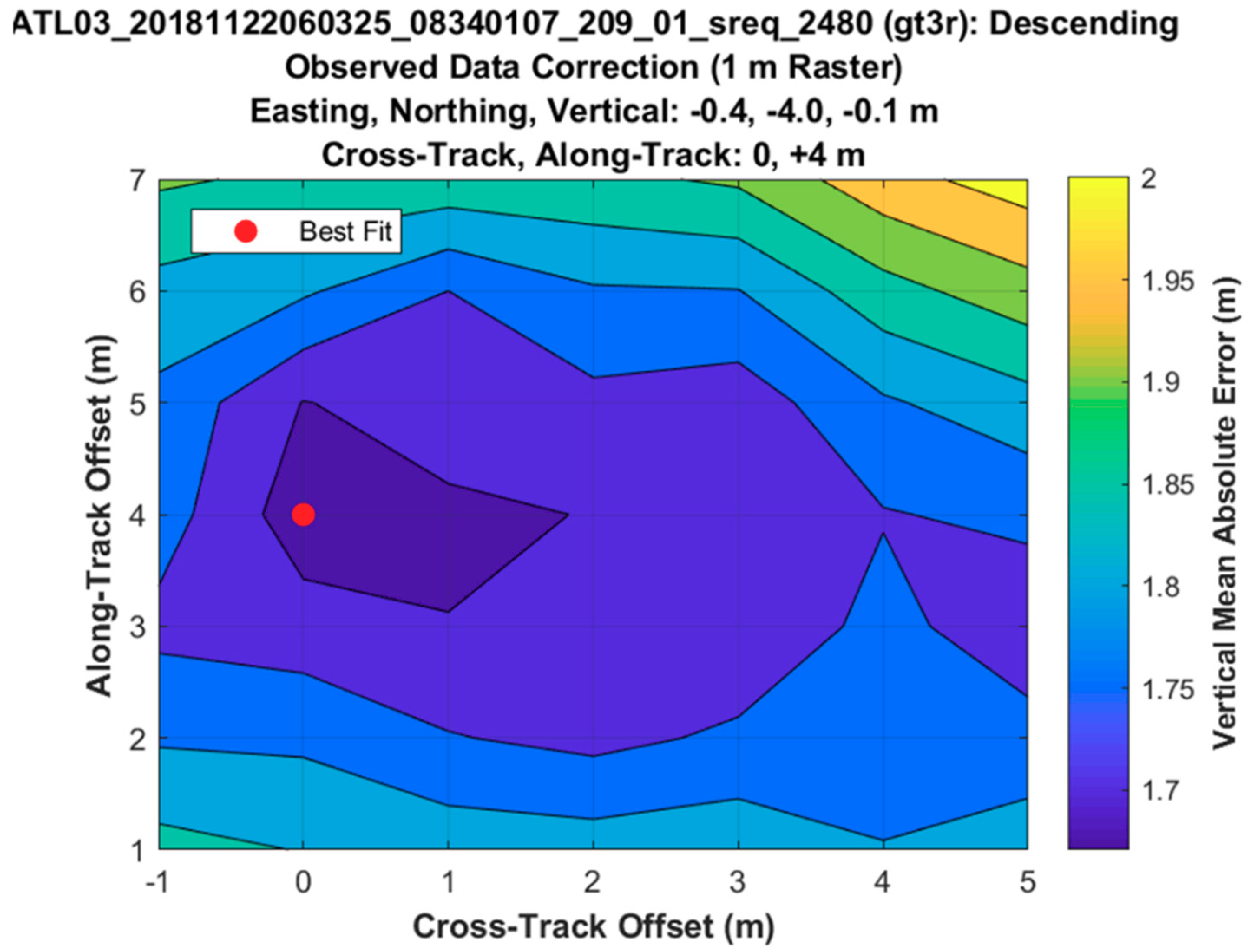
3. Results
4. Discussion
5. Conclusions
Author Contributions
Funding
Acknowledgments
Conflicts of Interest
References
- National Oceanic and Atmospheric Administration (NOAA): Field Procedures Manual. Available online: https://nauticalcharts.noaa.gov/publications/docs/standards-and-requirements/fpm/2014-fpm-final.pdf (accessed on 21 May 2019).
- Plant, N.G.; Holland, K.T.; Puleo, J.A. Analysis of the scale of errors in nearshore bathymetric data. Mar. Geol. 2002, 191, 71–86. [Google Scholar] [CrossRef]
- Titov, V.V.; Gonzalez, F.I.; Bernard, E.N.; Eble, M.C.; Mofjeld, H.O.; Newman, J.C.; Venturato, A.J. Real-time tsunami forecasting: Challenges and solutions. Nat. Hazards 2005, 35, 35–41. [Google Scholar] [CrossRef]
- Costa, B.M.; Battista, T.A.; Pittman, S.J. Comparative evaluation of airborne LiDAR and ship-based multibeam SoNAR bathymetry and intensity for mapping coral reef ecosystems. Remote Sens. Environ. 2009, 113, 1082–1100. [Google Scholar] [CrossRef]
- Gao, J. Bathymetric mapping by means of remote sensing: Methods, accuracy and limitations. Prog. Phys. Geogr. 2009, 33, 103–116. [Google Scholar] [CrossRef]
- Polcyn, F.C.; Lyzenga, D.R. Remote Bathymetry and Shoal Detection with ERTS: ERTS Water Depth; NASA Technical Reports, ERIM Report No. 193300-51-F; National Aeronautics and Space Administration: Washington, DC, USA, 1975. [Google Scholar]
- Lyzenga, D.R.; Polcyn, F.C. Techniques for the Extraction of Water Depth Information from Landsat Digital Data (No. ERIM-129900-1-F); Environmental Research Institute of Michigan Ann Arbor Applications Div.: Ann Arbor, MI, USA, 1979. [Google Scholar]
- Arsen, A.; Crétaux, J.F.; Berge-Nguyen, M.; Del Rio, R. Remote sensing-derived bathymetry of lake Poopó. Remote Sens. 2014, 6, 407–420. [Google Scholar] [CrossRef]
- Markus, T.; Neumann, T.; Martino, A.; Abdalati, W.; Brunt, K.; Csatho, B.; Farrell, S.; Fricker, H.; Gardner, A.; Harding, D.; et al. The Ice, Cloud, and land Elevation Satellite-2 (ICESat-2): Science requirements, concept, and implementation. Remote Sens. Environ. 2017, 190, 260–273. [Google Scholar] [CrossRef]
- Palm, S.; Yang, Y.; Herzfeld, U. ICESat-2 Algorithm Theoretical Basis Document for the Atmosphere, Part I: Level 2 and 3 Data Products. National Aeronautics and Space Administration, Goddard Space Flight Center, 2018. Available online: https://icesat-2.gsfc.nasa.gov/sites/default/files/files/ATL04_ATL09_15June2018.pdf (accessed on 21 May 2019).
- Magruder, L.A.; Brunt, K.M. Performance analysis of airborne photon-counting lidar data in preparation for the ICESat-2 mission. IEEE Trans. Geosci. Remote Sens. 2018, 56, 2911–2918. [Google Scholar] [CrossRef]
- Philpot, W.D. Bathymetric mapping with passive multispectral imagery. Appl. Opt. 1989, 28, 1569–1578. [Google Scholar] [CrossRef]
- Liceaga-Correa, M.A.; Euan-Avila, J.I. Assessment of coral reef bathymetric mapping using visible Landsat Thematic Mapper data. Int. J. Remote Sens. 2002, 23, 3–14. [Google Scholar] [CrossRef]
- Stumpf, R.P.; Holderied, K.; Sinclair, M. Determination of water depth with high-resolution satellite imagery over variable bottom types. Limnol. Oceanogr. 2003, 48, 547–556. [Google Scholar] [CrossRef]
- Dierssen, H.M.; Zimmerman, R.C.; Leathers, R.A.; Downes, T.V.; Davis, C.O. Ocean color remote sensing of seagrass and bathymetry in the Bahamas Banks by high-resolution airborne imagery. Limnol. Oceanogr. 2003, 48, 444–455. [Google Scholar] [CrossRef]
- Lyzenga, D.R.; Malinas, N.P.; Tanis, F.J. Multispectral bathymetry using a simple physically based algorithm. IEEE Trans. Geosci. Remote Sens. 2006, 44, 2251–2259. [Google Scholar] [CrossRef]
- Forfinski-Sarkozi, N.A.; Parrish, C.E. Active-Passive Spaceborne Data Fusion for Mapping Nearshore Bathymetry. Photogramm. Eng. Remote Sens. 2019, 85, 281–295. [Google Scholar] [CrossRef]
- Forfinski-Sarkozi, N.; Parrish, C. Analysis of MABEL bathymetry in Keweenaw bay and implications for ICESat-2 ATLAS. Remote Sens. 2016, 8, 772. [Google Scholar] [CrossRef]
- Jasinski, M.F.; Stoll, J.D.; Cook, W.B.; Ondrusek, M.; Stengel, E.; Brunt, K. Inland and near-shore water profiles derived from the high-altitude Multiple Altimeter Beam Experimental Lidar (MABEL). J. Coast. Res. 2016, 76, 44–55. [Google Scholar] [CrossRef]
- Neumann, T.; Brenner, A.; Hancock, D.; Robbins, J.; Saba, J.; Harbeck, K. ICE, CLOUD, and Land Elevation Satellite-2 (ICESat-2) Project: Algorithm Theoretical Basis Document (ATBD) for Global Geolocated Photons: ATL03. National Aeronautics and Space Administration, Goddard Space Flight Center. Available online: https://icesat-2.gsfc.nasa.gov/sites/default/files/files/ATL03_05June2018.pdf (accessed on 21 May 2019).
- Mobley, C.D. The optical properties of water. In Handbook of Optics, Vol I; The Optical Society of America (OSA), McGraw-Hill: New York, NY, USA, 1995; pp. 43.3–43.56. [Google Scholar]
- Neuenschwander, A.; Magruder, L. The potential impact of vertical sampling uncertainty on ICESat-2/ATLAS terrain and canopy height retrievals for multiple ecosystems. Remote Sens. 2016, 8, 1039. [Google Scholar] [CrossRef]
- Quadros, N.D. Unlocking the Characteristics of Bathymetric Lidar Sensors. LiDAR Mag. 2013, 3, 62–67. [Google Scholar]
- Doneus, M.; Miholjek, I.; Mandlburger, G.; Doneus, N.; Verhoeven, G.; Briese, C.; Pregesbauer, M. Airborne laser bathymetry for documentation of submerged archaeological sites in shallow water. In Proceedings of the Underwater 3D Recording and Modeling, ISPRS, Piano di Sorrento, Italy, 16–17 April 2015; pp. 99–107. [Google Scholar]
- Schwarz, R.; Pfeifer, N.; Pfennigbauer, M.; Ullrich, A. Exponential decomposition with implicit deconvolution of lidar backscatter from the water column. PFG J. Photogramm. Remote Sens. Geoinf. Sci. 2017, 85, 159–167. [Google Scholar] [CrossRef]
- Mandlburger, G.; Hauer, C.; Wieser, M.; Pfeifer, N. Topo-bathymetric LiDAR for monitoring river morphodynamics and instream habitats—A case study at the Pielach River. Remote Sens. 2015, 7, 6160–6195. [Google Scholar] [CrossRef]
- Cooper, C.; Faux, R.; White, S. Mapping Coastal South Carolina: Topo-Bathymetric Acquisition and Processing Strategies for Complex Near-Shore Environments. In Proceedings of the the 18th Annual Coastal Mapping & Charting Workshop of the Joint Airborne Lidar Bathymetry Technical Center of Expertise (JALBTCX), Savannah, GA, USA, 6–8 June 2017. [Google Scholar]
- Pittman, S.; Bauer, L.J.; Hile, S.; Jeffrey, C.F.; Davenport, E.D.; Caldow, C. Marine Protected Areas of the US Virgin Islands: Ecological Performance Report. Available online: https://repository.library.noaa.gov/view/noaa/880 (accessed on 21 May 2019).
- Department of Planning and Natural Resources and United States Department of Agriculture. Unified Watershed Assessment Report: United States Virgin Islands. Available online: http://ufdcimages.uflib.ufl.edu/CA/01/30/06/81/00001/UWA.pdf (accessed on 21 May 2019).
- Rothenberger, P.; Blondeau, J.; Cox, C.; Curtis, S.; Fisher, W.S.; Garrison, V.; Hillis-Starr, Z.; Jeffrey, C.F.; Kadison, E.; Lundgren, I.; et al. The state of coral reef ecosystems of the US Virgin Islands. In The State of Coral Reef Ecosystems of the United States and Pacific Freely Associated States 2008; National Centers for Coastal Ocean Science: Silver Spring, MD, USA, 2019; Volume 73, pp. 29–73. [Google Scholar]
- Soffer, N.; Brandt, M.E.; Correa, A.M.; Smith, T.B.; Thurber, R.V. Potential role of viruses in white plague coral disease. ISME J. 2014, 8, 271. [Google Scholar] [CrossRef]
- Wilson, N.; Parrish, C.E.; Battista, T.; Wright, C.W.; Costa, B.; Slocum, R. New Algorithms and Techniques for Mapping Benthic Composition with the EAARL-B Topo-bathymetric Lidar. Estuar. Coasts, under review.
- Wright, C.W.; Kranenburg, C.; Battista, T.A.; Parrish, C. Depth calibration and validation of the Experimental Advanced Airborne Research LIDAR, EAARL-B. J. Coast. Res. 2016, 76, 4–17. [Google Scholar] [CrossRef]
- Slocum, R.K.; Oregon State University, Corvallis, OR, USA. Personal communication, 2019.
- Raber, S. United States Virgin Islands Lidar Data Acquisition and Processing Post-Flight Aerial Acquisition and Calibration Report. National Oceanic and Atmospheric Administration. Available online: https://coast.noaa.gov/htdata/lidar2_z/geoid12b/data/3669/supplemental/usvi2013_stc_stj_stt_m3669_post_flight_report.pdf (accessed on 21 May 2019).
- Wang, M.; Son, S.; Harding, L.W., Jr. Retrieval of diffuse attenuation coefficient in the Chesapeake Bay and turbid ocean regions for satellite ocean color applications. J. Geophys. Res. Oceans 2009, 114, 1–15. [Google Scholar] [CrossRef]
- Feygels, V.I.; Optech International, Kiln, MS, USA. Personal communication, 2019.
- Hojerslev, N.K. Visibility of the sea with special reference to the Secchi disc. In Proceedings of the Ocean Optics VIII: International Society for Optics and Photonics, Orlando, FL, USA, 7 August 1986; Volume 637, pp. 294–308. [Google Scholar]
- Feygels, V.I.; Kopilevich, Y.; Park, J.Y.; Kim, M.; Aitken, J. Particularities of hydro lidar missions in the Asia-Pacific region. In Proceedings of the Lidar Remote Sensing for Environmental Monitoring XIV, International Society for Optics and Photonics, Beijing, China, 13–16 October 2014; Volume 9262, p. 92620X. [Google Scholar]
- Gordon, H.R.; Wouters, A.W. Some relationships between Secchi depth and inherent optical properties of natural waters. Appl. Opt. 1978, 17, 3341–3343. [Google Scholar] [CrossRef] [PubMed]
- Guenther, G.C. Airborne Laser Hydrography: System Design and Performance Factors; National Oceanic and Atmospheric Administration: Rockville, MD, USA, 1985; pp. 23–40. [Google Scholar]
- Marin, F.; Rohatgi, A.; Charlot, S. WebPlotDigitizer, a polyvalent and free software to extract spectra from old astronomical publications: Application to ultraviolet spectropolarimetry. arXiv 2017, arXiv:1708.02025. [Google Scholar]
- Neumann, T.; NASA, Greenbelt, MD, USA. Personal communication 2019.
- Wang, X.; Glennie, C.; Pan, Z. Weak Echo Detection from Single Photon Lidar Data Using a Rigorous Adaptive Ellipsoid Searching Algorithm. Remote Sens. 2018, 10, 1035. [Google Scholar] [CrossRef]


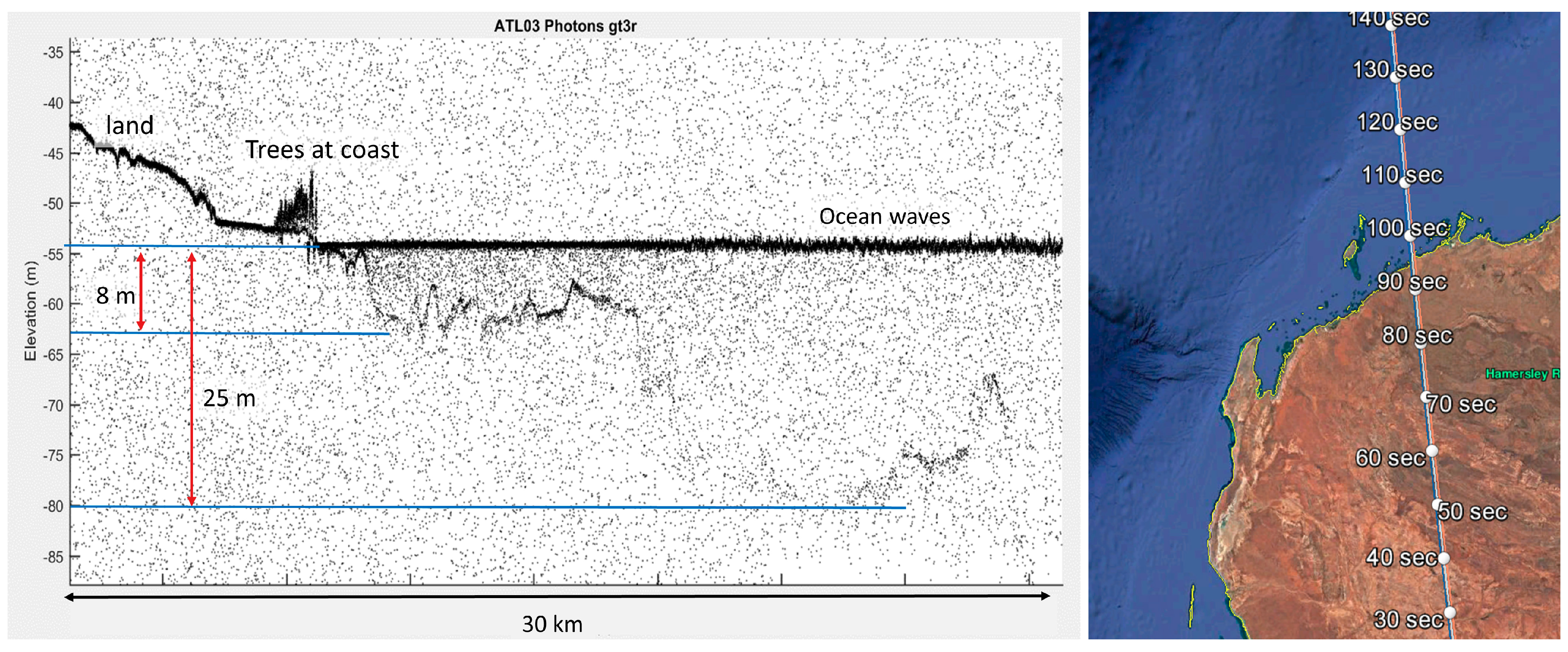
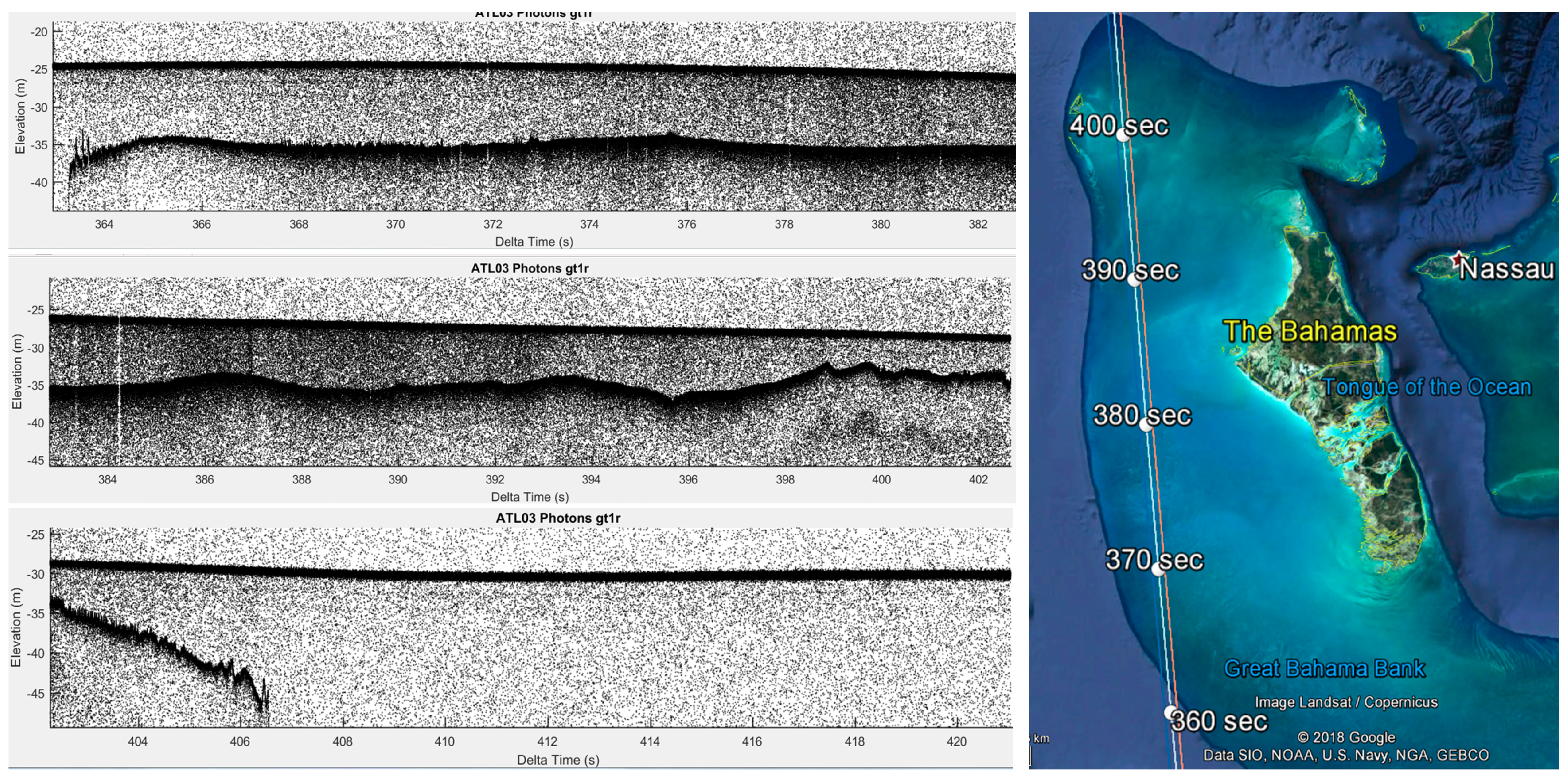
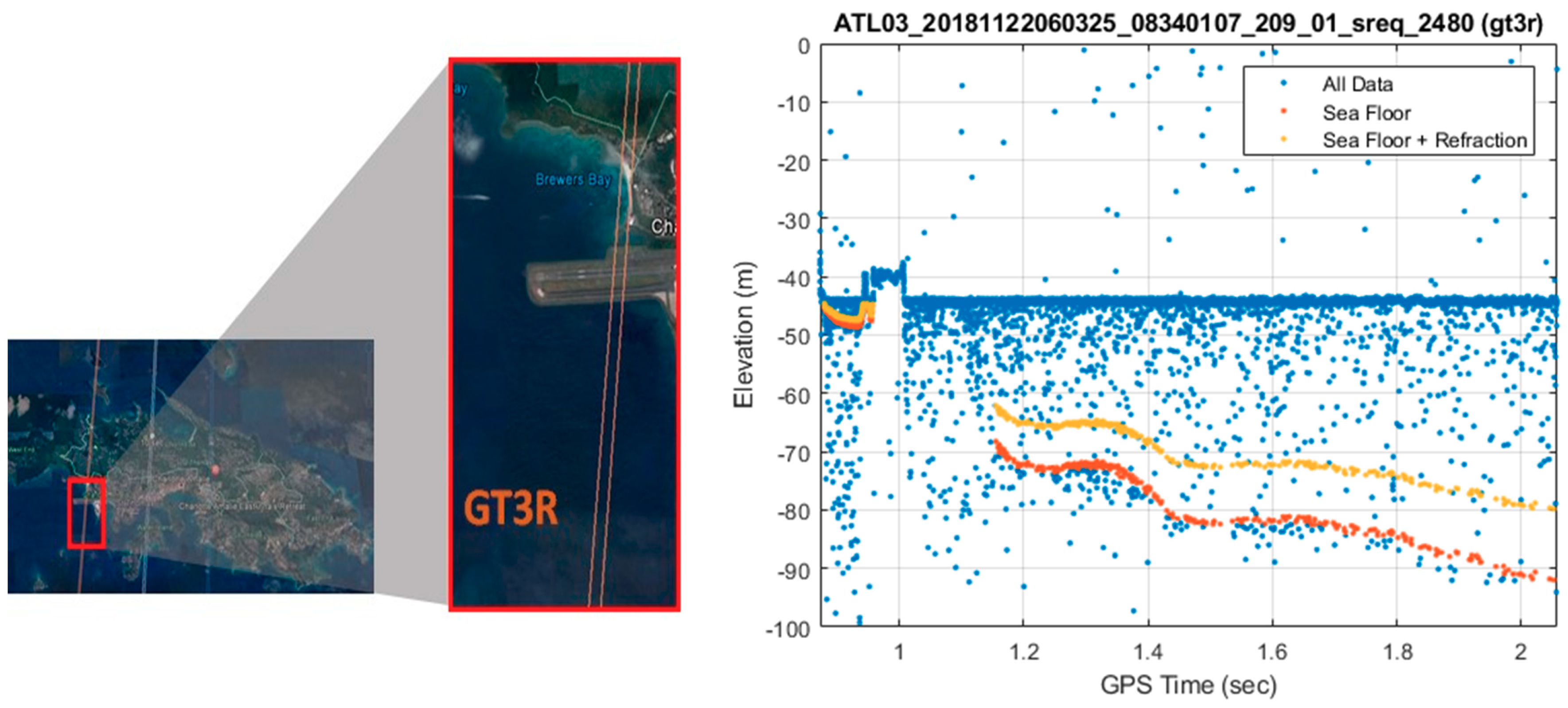
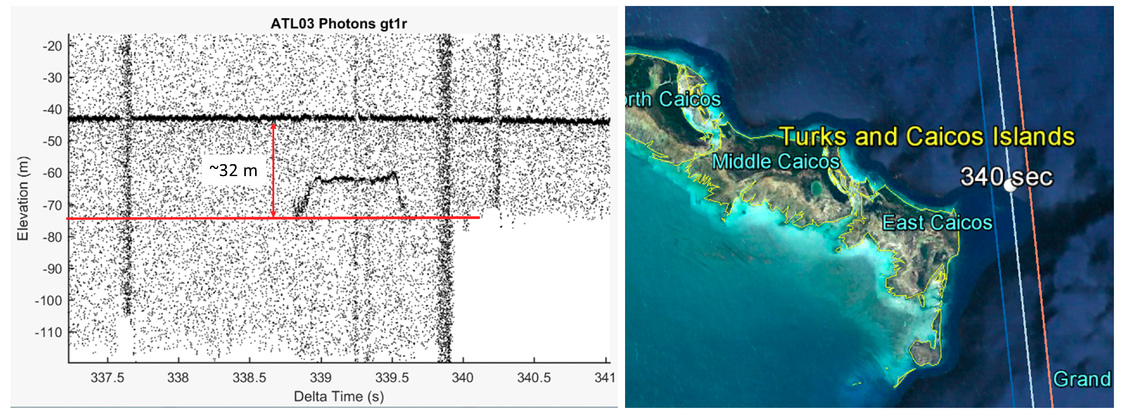
| Site | Date of ICESat-2 Overpass | Maximum Observed Depths (Refraction Corrected), Dmax [m] | |
|---|---|---|---|
| Turks and Caicos | 21°42′12″ N, 71°22′50″ W | 10/19/2018 (Julian day 292) | 24 |
| North West Australia (western Pilbara region) | 20°41′40″ S, 116°06′55″ E | 10/18/2018 (Julian day 291) | 19 |
| Great Bahama Bank | 24°42′46″ N, 78°54′21″ W | 10/26/2018 (Julian day 299) | 13 |
| St. Thomas | 18°19′35″ N, 64°58′43″ W | 11/22/2018 (Julian day 326) | 38 |
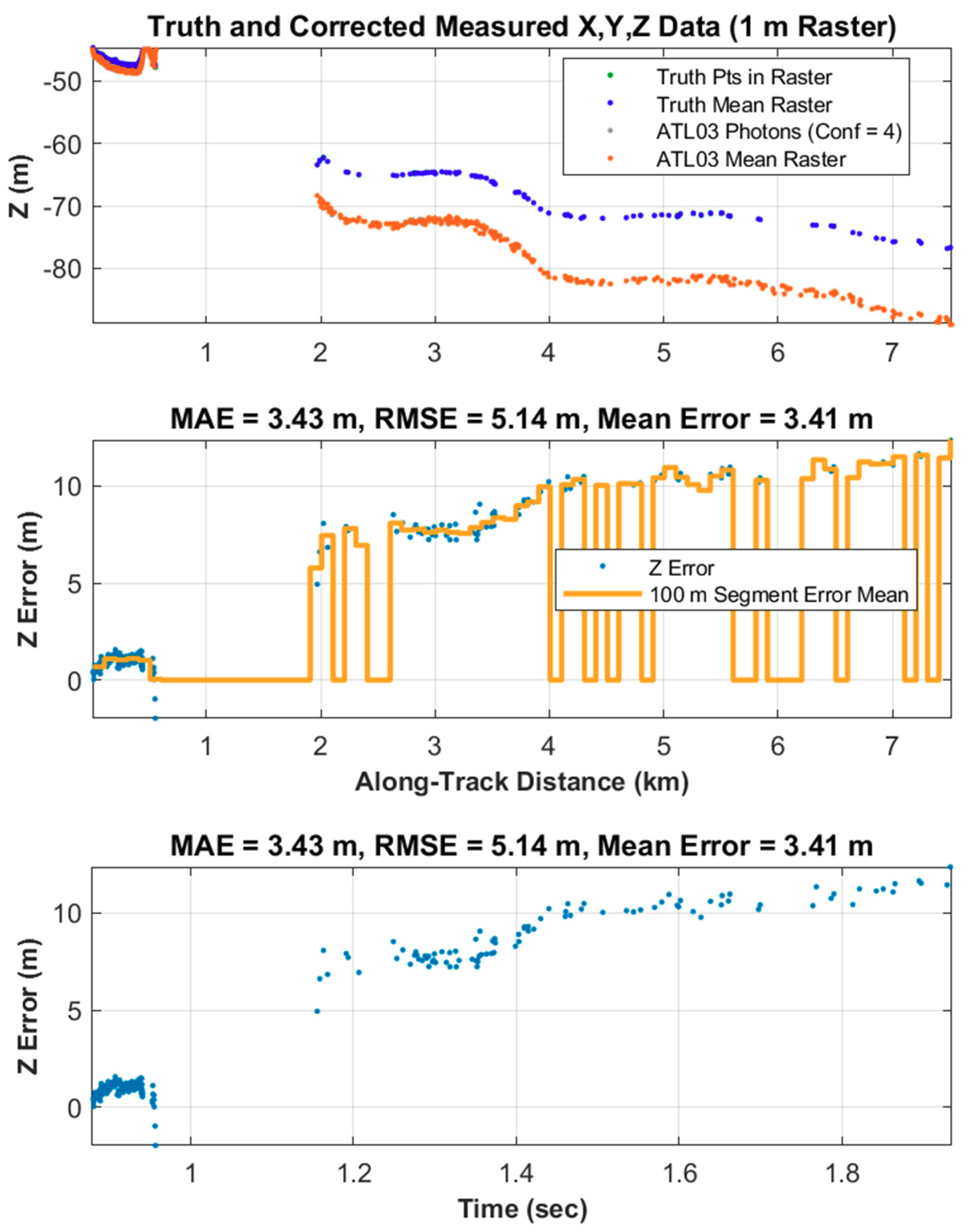
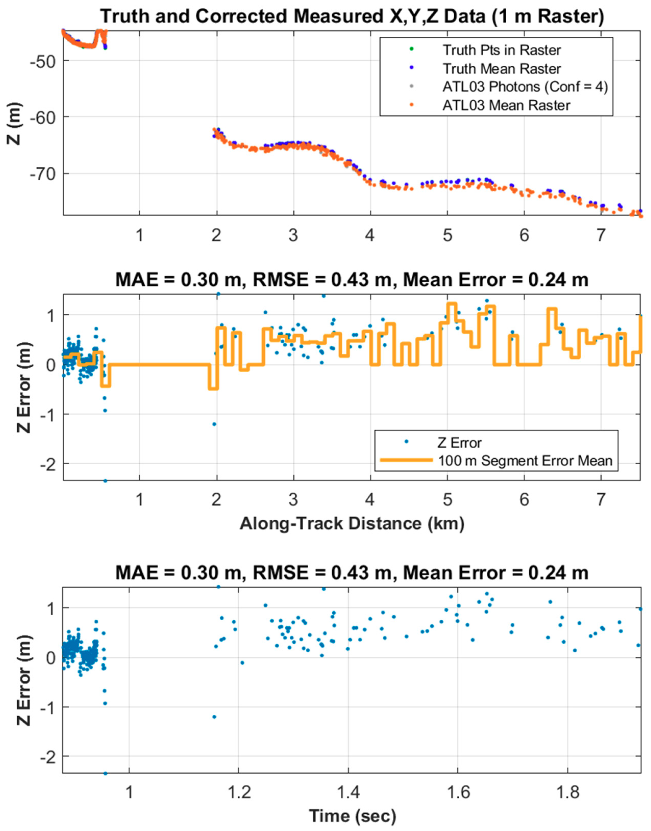
| Track | Description of Track | MAE (m) | RMSE (m) | Mean Error (m) |
|---|---|---|---|---|
| GT2L | Weak beam of center beam pair | 0.44 | 0.56 | 0.00 |
| GT2R | Strong beam of center beam pair | 0.41 | 0.60 | -0.12 |
| GT3L | Weak beam of right beam pair | 0.36 | 0.43 | 0.17 |
| GT3R | Strong beam of right beam pair | 0.30 | 0.43 | 0.24 |
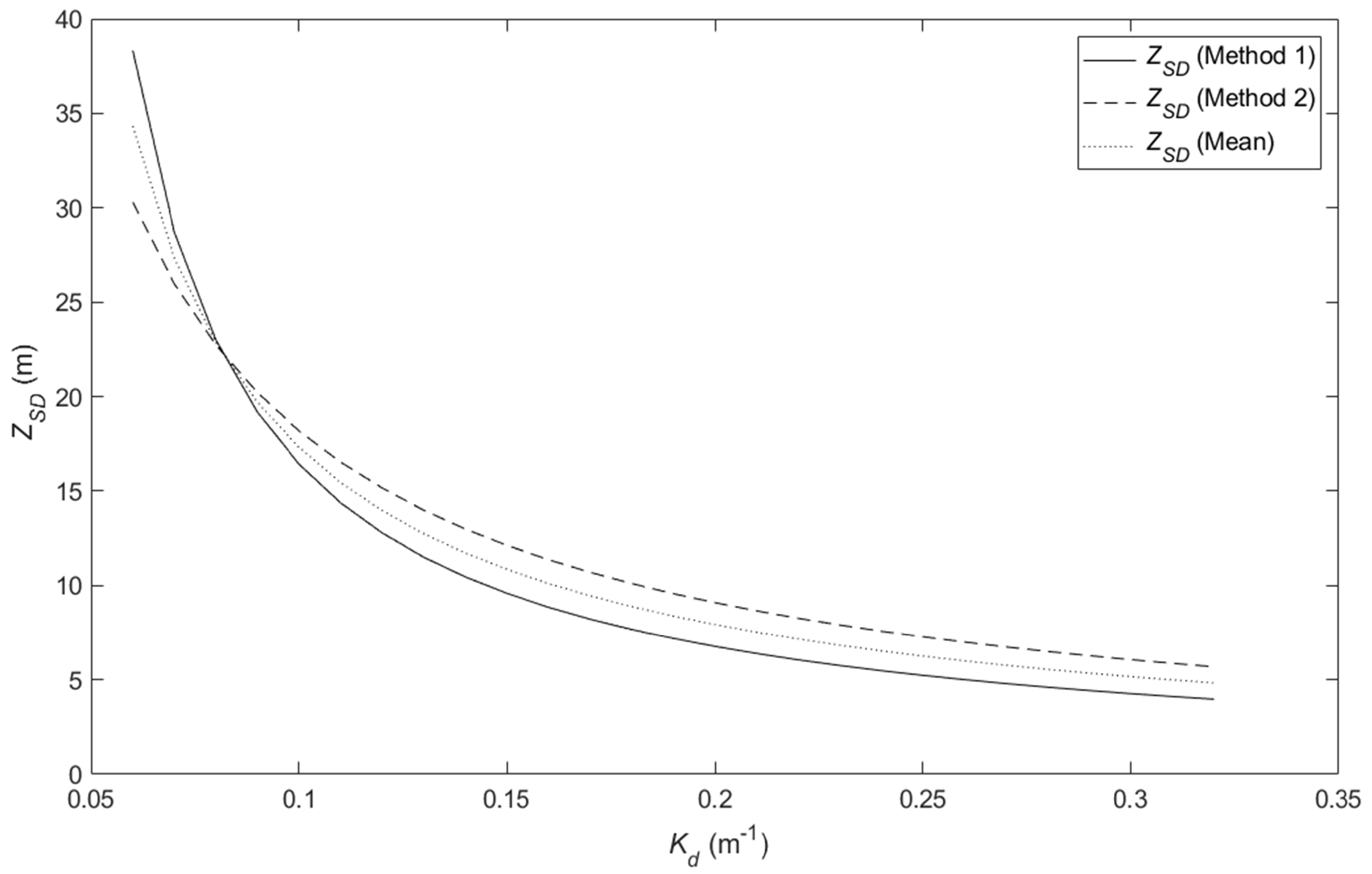
| Site | Maximum Depth, Dmax [m] | VIIRS Kd(490) [m−1] | Secchi Depth, ZSD [m] | Max Depth Penetration in Secchi Depths | Maximum Optical Depth, KdDmax |
|---|---|---|---|---|---|
| Turks and Caicos | 24 | 0.075 | 25.1 | 0.95 | 1.79 |
| North West Australia (western Pilbara region) | 19 | 0.099 | 17.6 | 1.08 | 1.87 |
| Great Bahama Bank | 13 | 0.123 | 13.6 | 0.96 | 1.60 |
| St. Thomas | 38 | 0.053 | 32.1 | 0.84 | 2.01 |
| Mean | 24 | 0.087 | 22.1 | 0.96 | 1.82 |
© 2019 by the authors. Licensee MDPI, Basel, Switzerland. This article is an open access article distributed under the terms and conditions of the Creative Commons Attribution (CC BY) license (http://creativecommons.org/licenses/by/4.0/).
Share and Cite
Parrish, C.E.; Magruder, L.A.; Neuenschwander, A.L.; Forfinski-Sarkozi, N.; Alonzo, M.; Jasinski, M. Validation of ICESat-2 ATLAS Bathymetry and Analysis of ATLAS’s Bathymetric Mapping Performance. Remote Sens. 2019, 11, 1634. https://doi.org/10.3390/rs11141634
Parrish CE, Magruder LA, Neuenschwander AL, Forfinski-Sarkozi N, Alonzo M, Jasinski M. Validation of ICESat-2 ATLAS Bathymetry and Analysis of ATLAS’s Bathymetric Mapping Performance. Remote Sensing. 2019; 11(14):1634. https://doi.org/10.3390/rs11141634
Chicago/Turabian StyleParrish, Christopher E., Lori A. Magruder, Amy L. Neuenschwander, Nicholas Forfinski-Sarkozi, Michael Alonzo, and Michael Jasinski. 2019. "Validation of ICESat-2 ATLAS Bathymetry and Analysis of ATLAS’s Bathymetric Mapping Performance" Remote Sensing 11, no. 14: 1634. https://doi.org/10.3390/rs11141634
APA StyleParrish, C. E., Magruder, L. A., Neuenschwander, A. L., Forfinski-Sarkozi, N., Alonzo, M., & Jasinski, M. (2019). Validation of ICESat-2 ATLAS Bathymetry and Analysis of ATLAS’s Bathymetric Mapping Performance. Remote Sensing, 11(14), 1634. https://doi.org/10.3390/rs11141634