Canopy Height Layering Biomass Estimation Model (CHL-BEM) with Full-Waveform LiDAR


 ,
, 
Abstract

1. Introduction
2. Materials
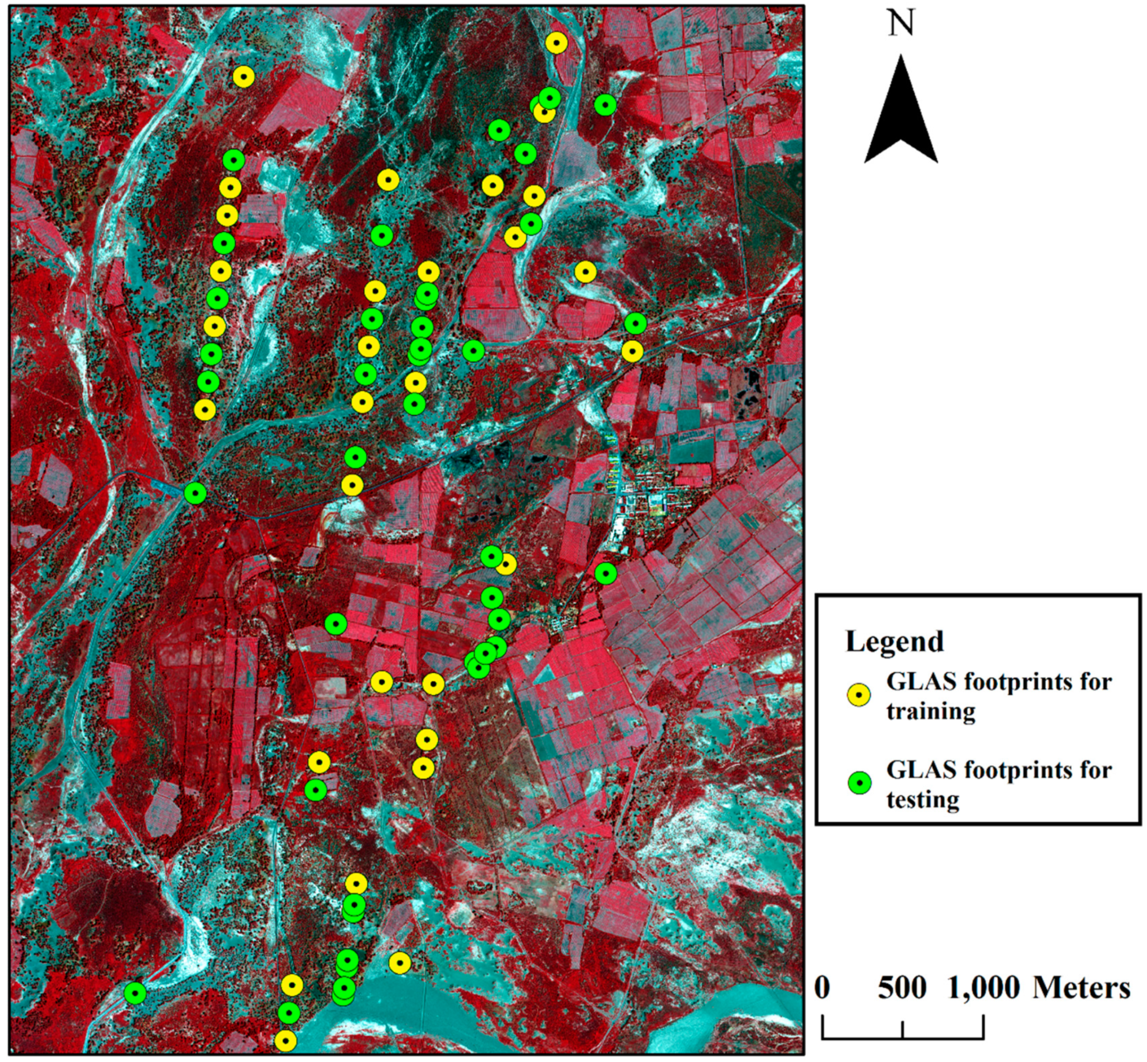
2.1. Study Site
2.2. GLAS Data
2.3. Field Biomass
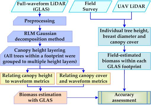
3. Methods
3.1. GLAS Preprocessing
3.2. RLM Gaussian Decomposition Method
3.3. Canopy Height Layering Biomass Estimation Model (CHL-BEM)
3.3.1. Canopy Height and Canopy Cover
3.3.2. Biomass Estimation
3.4. Two Other Biomass Models for Comparison
4. Results and Discussion
4.1. CHL-BEM Estimated Biomass
4.2. CHL-BEM vs. Other Two Biomass Models
- (1).
- The CTH-BEM obtained the lowest accuracy among the three models. This was mainly caused by the distribution characteristics of Populus euphratica in the horizontal and vertical directions. In the vertical direction, the height of Populus euphratica ranges from 5 to 19 m within some GLAS footprints. The CTH-BEM only utilizes the maximum height for biomass estimation, which leads to poor accuracy. In the horizontal direction, the spatial distribution of Populus euphratica is quite sparse and uneven. Canopy cover not being considered in the CTH-BEM also leads to a poor biomass estimation accuracy. Therefore, the canopy height layering methods for both canopy height and canopy cover must be considered to address the abovementioned issues.
- (2).
- The CTH&CC-BEM obtained a relatively higher accuracy than the CTH-BEM, but it was still not ideal. Results showed that the CTH&CC-BEM gained a higher accuracy than the CTH-BEM, which was mainly because the canopy cover was considered as an additional key input parameter. As we all know, breast diameter is a key indicator of biomass estimation, but we cannot acquire this information from GLAS data. Some existing research has confirmed that a positive correlation exists between canopy cover and breast diameter [17,52,53]. Therefore, considering the canopy cover improved the biomass estimation results.
- (3).
- The CHL-BEM obtained the highest accuracy among the three models. Though there still exist some limitations, as mentioned in Section 4.1, it achieved a satisfactory accuracy in biomass estimation. This was mainly because the CHL-BEM divided all trees within a GLAS footprint into multiple height layers and used the layered canopy height and canopy cover for biomass estimation. Therefore, we suggest that canopy height layering methods should be further explored to improve forest biomass estimation accuracy in future work. The newly developed CHL-BEM can be applied on other full-waveform LiDAR data such as GEDI.
5. Conclusions
Author Contributions
Funding
Acknowledgments
Conflicts of Interest
References
- Houghton, R.A. Aboveground Forest Biomass and the Global Carbon Balance. Glob. Chang. Biol. 2010, 11, 945–958. [Google Scholar] [CrossRef]
- Fayad, I.; Baghdadi, N.; Guitet, S.; Bailly, J.-S.; Hérault, B.; Gond, V.; El Hajj, M.; Tong Minh, D.H. Aboveground biomass mapping in French Guiana by combining remote sensing, forest inventories and environmental data. Int. J. Appl. Earth Obs. Geoinf. 2016, 52, 502–514. [Google Scholar] [CrossRef]
- Baccini, A.; Laporte, N.; Goetz, S.J.; Sun, M.; Dong, H. A first map of tropical Africa’s above-ground biomass derived from satellite imagery. Environ. Res. Lett. 2008, 3, 045011. [Google Scholar] [CrossRef]
- Clark, M.L.; Roberts, D.A.; Ewel, J.J.; Clark, D.B. Estimation of tropical rain forest aboveground biomass with small-footprint lidar and hyperspectral sensors. Remote Sens. Environ. 2011, 115, 2931–2942. [Google Scholar] [CrossRef]
- Zhang, G.; Ganguly, S.; Nemani, R.R.; White, M.A.; Milesi, C.; Hashimoto, H.; Wang, W.; Saatchi, S.; Yu, Y.; Myneni, R.B. Estimation of forest aboveground biomass in California using canopy height and leaf area index estimated from satellite data. Remote Sens. Environ. 2014, 151, 44–56. [Google Scholar] [CrossRef]
- Zhang, X.; Kondragunta, S. Estimating forest biomass in the USA using generalized allometric models and MODIS land products. Geophys. Res. Lett. 2006, 33. [Google Scholar] [CrossRef]
- Zolkos, S.G.; Goetz, S.J.; Dubayah, R. A meta-analysis of terrestrial aboveground biomass estimation using lidar remote sensing. Remote Sens. Environ. 2013, 128, 289–298. [Google Scholar] [CrossRef]
- Ballhorn, U.; Jubanski, J.; Siegert, F. ICESat/GLAS Data as a Measurement Tool for Peatland Topography and Peat Swamp Forest Biomass in Kalimantan, Indonesia. Remote Sens. 2011, 3, 1957–1982. [Google Scholar] [CrossRef]
- Wulder, M.A.; White, J.C.; Nelson, R.F.; Næsset, E.; Ørka, H.O.; Coops, N.C.; Hilker, T.; Bater, C.W.; Gobakken, T. Lidar sampling for large-area forest characterization: A review. Remote Sens. Environ. 2012, 121, 196–209. [Google Scholar] [CrossRef]
- Greaves, H.E.; Vierling, L.A.; Eitel, J.U.H.; Boelman, N.T.; Magney, T.S.; Prager, C.M.; Griffin, K.L. High-resolution mapping of aboveground shrub biomass in Arctic tundra using airborne lidar and imagery. Remote Sens. Environ. 2016, 184, 361–373. [Google Scholar] [CrossRef]
- Gregoire, T.G.; Næsset, E.; McRoberts, R.E.; Ståhl, G.; Andersen, H.-E.; Gobakken, T.; Ene, L.; Nelson, R. Statistical rigor in LiDAR-assisted estimation of aboveground forest biomass. Remote Sens. Environ. 2016, 173, 98–108. [Google Scholar] [CrossRef]
- Hajj, M.E.; Baghdadi, N.; Fayad, I.; Vieilledent, G.; Bailly, J.-S.; Minh, D.H.T. Interest of Integrating Spaceborne LiDAR Data to Improve the Estimation of Biomass in High Biomass Forested Areas. Remote Sens. 2017, 9, 213. [Google Scholar]
- Lefsky, M.A.; Cohen, W.B.; Harding, D.J.; Parker, G.G.; Acker, S.A.; Gower, S.T. Lidar remote sensing of above-ground biomass in three biomes. Glob. Ecol. Biogeogr. 2002, 11, 393–399. [Google Scholar] [CrossRef]
- Margolis, H.A.; Nelson, R.F.; Montesano, P.M.; Beaudoin, A.; Sun, G.; Andersen, H.-E.; Wulder, M.A. Combining satellite lidar, airborne lidar, and ground plots to estimate the amount and distribution of aboveground biomass in the boreal forest of North America 1. Can. J. For. Res. 2015, 45, 838–855. [Google Scholar] [CrossRef]
- Montesano, P.M.; Nelson, R.F.; Dubayah, R.O.; Sun, G.; Cook, B.D.; Ranson, K.J.R.; Næsset, E.; Kharuk, V. The uncertainty of biomass estimates from LiDAR and SAR across a boreal forest structure gradient. Remote Sens. Environ. 2014, 154, 398–407. [Google Scholar] [CrossRef]
- Nelson, R.; Margolis, H.; Montesano, P.; Sun, G.; Cook, B.; Corp, L.; Andersen, H.E.; Dejong, B.; Pellat, F.P.; Fickel, T. Lidar-based estimates of aboveground biomass in the continental US and Mexico using ground, airborne, and satellite observations. Remote Sens. Environ. 2017, 188, 127–140. [Google Scholar] [CrossRef]
- Popescu, S.C.; Wynne, R.H.; Nelson, R.F. Measuring individual tree crown diameter with lidar and assessing its influence on estimating forest volume and biomass. Can. J. Remote Sens. 2003, 29, 564–577. [Google Scholar] [CrossRef]
- Popescu, S.C.; Zhao, K.; Neuenschwander, A.; Lin, C. Satellite lidar vs. small footprint airborne lidar: Comparing the accuracy of aboveground biomass estimates and forest structure metrics at footprint level. Remote Sens. Environ. 2011, 115, 2786–2797. [Google Scholar] [CrossRef]
- Chi, H.; Sun, G.; Huang, J.; Guo, Z.; Ni, W.; Fu, A. National Forest Aboveground Biomass Mapping from ICESat/GLAS Data and MODIS Imagery in China. Remote Sens. 2015, 7, 5534–5564. [Google Scholar] [CrossRef]
- Fatoyinbo, T.E.; Simard, M. Height and biomass of mangroves in Africa from ICESat/GLAS and SRTM. Int. J. Remote Sens. 2013, 34, 668–681. [Google Scholar] [CrossRef]
- Zhang, Y.; Liang, S.; Sun, G. Forest biomass mapping of northeastern China using GLAS and MODIS data. IEEE J. Sel. Top. Appl. Earth Obs. Remote Sens. 2014, 7, 140–152. [Google Scholar] [CrossRef]
- Nie, S.; Wang, C.; Xi, X.; Luo, S.; Li, G.; Tian, J.; Wang, H. Estimating the vegetation canopy height using micro-pulse photon-counting LiDAR data. Opt. Express 2018, 26, A520–A540. [Google Scholar] [CrossRef] [PubMed]
- Hong, C.; Sun, G.; Huang, J.; Li, R.; Ren, X.; Ni, W.; Fu, A. Estimation of Forest Aboveground Biomass in Changbai Mountain Region Using ICESat/GLAS and Landsat/TM Data. Remote Sens. 2017, 9, 707. [Google Scholar]
- Liu, K.; Wang, J.; Zeng, W.; Song, J. Comparison and Evaluation of Three Methods for Estimating Forest above Ground Biomass Using TM and GLAS Data. Remote Sens. 2017, 9, 341. [Google Scholar]
- Shen, W.; Li, M.; Huang, C.; Xin, T.; Wei, A. Annual forest aboveground biomass changes mapped using ICESat/GLAS measurements, historical inventory data, and time-series optical and radar imagery for Guangdong province, China. Agric. For. Meteorol. 2018, 259, 23–38. [Google Scholar] [CrossRef]
- Dolan, K.A.; Hurtt, G.C.; Chambers, J.Q.; Dubayah, R.O.; Frolking, S.; Masek, J.G. Using ICESat’s Geoscience Laser Altimeter System (GLAS) to assess large-scale forest disturbance caused by hurricane Katrina. Remote Sens. Environ. 2011, 115, 86–96. [Google Scholar] [CrossRef]
- Duncanson, L.I.; Niemann, K.O.; Wulder, M.A. Estimating forest canopy height and terrain relief from GLAS waveform metrics. Remote Sens. Environ. 2010, 114, 138–154. [Google Scholar] [CrossRef]
- García, M.; Popescu, S.; Riaño, D.; Zhao, K.; Neuenschwander, A.; Agca, M.; Chuvieco, E. Characterization of canopy fuels using ICESat/GLAS data. Remote Sens. Environ. 2012, 123, 81–89. [Google Scholar] [CrossRef]
- Tang, H.; Dubayah, R.; Brolly, M.; Ganguly, S.; Zhang, G. Large-scale retrieval of leaf area index and vertical foliage profile from the spaceborne waveform lidar (GLAS/ICESat). Remote Sens. Environ. 2014, 154, 8–18. [Google Scholar] [CrossRef]
- Nie, S.; Wang, C.; Zeng, H.; Xi, X.; Xia, S. A revised terrain correction method for forest canopy height estimation using ICESat/GLAS data. ISPRS J. Photogramm. Remote Sens. 2015, 108, 183–190. [Google Scholar] [CrossRef]
- Su, Y.; Guo, Q.; Xue, B.; Hu, T.; Alvarez, O.; Tao, S.; Fang, J. Spatial distribution of forest aboveground biomass in China: Estimation through combination of spaceborne lidar, optical imagery, and forest inventory data. Remote Sens. Environ. 2016, 173, 187–199. [Google Scholar] [CrossRef]
- Boudreau, J.; Nelson, R.; Margolis, H.; Beaudoin, A.; Guindon, L.; Kimes, D. Regional aboveground forest biomass using airborne and spaceborne LiDAR in Québec. Remote Sens. Environ. 2008, 112, 3876–3890. [Google Scholar] [CrossRef]
- Lefsky, M.A.; Harding, D.J.; Keller, M.; Cohen, W.B.; Carabajal, C.C.; Del Bom Espirito-Santo, F.; Hunter, M.O.; de Oliveira, R. Estimates of forest canopy height and aboveground biomass using ICESat. Geophys. Res. Lett. 2005, 32. [Google Scholar] [CrossRef]
- Nelson, R.; Ranson, K.J.; Sun, G.; Kimes, D.S.; Kharuk, V.; Montesano, P. Estimating Siberian timber volume using MODIS and ICESat/GLAS. Remote Sens. Environ. 2009, 113, 691–701. [Google Scholar] [CrossRef]
- Chen, Q. Retrieving vegetation height of forests and woodlands over mountainous areas in the Pacific Coast region using satellite laser altimetry. Remote Sens. Environ. 2010, 114, 1610–1627. [Google Scholar] [CrossRef]
- Zhong, H.P.; Liu, H.; Wang, Y.; Ya, T.; Geng, L.H.; Yan, Z.J. Relationship between Ejina oasis and water resources in the lower Heihe River basin. Adv. Water Sci. 2002, 13, 223–228. [Google Scholar]
- Tian, J.; Wang, L.; Li, X. Sub-footprint analysis to uncover tree height variation using ICESat/GLAS. Int. J. Appl. Earth Obs. Geoinf. 2015, 35, 284–293. [Google Scholar] [CrossRef]
- Sun, G.; Ranson, K.; Kimes, D.; Blair, J.; Kovacs, K. Forest vertical structure from GLAS: An evaluation using LVIS and SRTM data. Remote Sens. Environ. 2008, 112, 107–117. [Google Scholar] [CrossRef]
- Bogeat-Triboulot, M.-B.; Brosché, M.; Renaut, J.; Jouve, L.; Le Thiec, D.; Fayyaz, P.; Vinocur, B.; Witters, E.; Laukens, K.; Teichmann, T. Gradual soil water depletion results in reversible changes of gene expression, protein profiles, ecophysiology, and growth performance in Populus euphratica, a poplar growing in arid regions. Plant Physiol. 2007, 143, 876–892. [Google Scholar] [CrossRef]
- Dong, D.; Li, X.; Wan, H.; Lin, H. Aboveground biomass estimation of Populus euphratica in the lower reaches of Tarim River. J. Desert Res. 2013, 33, 724–730. [Google Scholar]
- Tian, J.; Wang, L.; Li, X.; Gong, H.; Shi, C.; Zhong, R.; Liu, X. Comparison of UAV and WorldView-2 imagery for mapping leaf area index of mangrove forest. Int. J. Appl. Earth Obs. Geoinf. 2017, 61, 22–31. [Google Scholar] [CrossRef]
- Tian, J.; Li, X.; Duan, F.; Wang, J.; Ou, Y. An Efficient Seam Elimination Method for UAV Images Based on Wallis Dodging and Gaussian Distance Weight Enhancement. Sensors 2016, 16, 662. [Google Scholar] [CrossRef] [PubMed]
- Yin, D.; Wang, L. Individual mangrove tree measurement using UAV-based LiDAR data: Possibilities and challenges. Remote Sens. Environ. 2019, 223, 34–49. [Google Scholar] [CrossRef]
- Tian, J.; Wang, L.; Li, X.; Shi, C.; Gong, H. Differentiating tree and shrub LAI in a mixed forest with ICESat/GLAS spaceborne LiDAR. IEEE J. Sel. Top. Appl. Earth Obs. Remote Sens. 2017, 10, 87–94. [Google Scholar] [CrossRef]
- Wang, X.; Huang, H.; Gong, P.; Liu, C.; Li, C.; Li, W. Forest canopy height extraction in rugged areas with ICESAT/GLAS data. IEEE Trans. Geosci. Remote Sens. 2014, 52, 4650–4657. [Google Scholar] [CrossRef]
- Wang, X.; Wu, J.; Lu, F.; Jiao, H.; Zhang, H. Optimal Selection of Algorisms for Denoising ICESat-GLAS Waveform Data and Development of a Forest Crown Height Estimation Model. Sci. Silvae Sin. 2017, 53, 62–72. [Google Scholar]
- Wang, Y.; Li, G.; Ding, J.; Guo, Z.; Tang, S.; Wang, C.; Huang, Q.; Liu, R.; Chen, J.M. A combined GLAS and MODIS estimation of the global distribution of mean forest canopy height. Remote Sens. Environ. 2016, 174, 24–43. [Google Scholar] [CrossRef]
- Miller, M.E.; Lefsky, M.; Pang, Y. Optimization of Geoscience Laser Altimeter System waveform metrics to support vegetation measurements. Remote Sens. Environ. 2011, 115, 298–305. [Google Scholar] [CrossRef]
- Los, S.O.; Rosette, J.A.B.; Kljun, N.; North, P.R.J.; Chasmer, L.; Suárez, J.C.; Hopkinson, C.; Hill, R.A.; van Gorsel, E.; Mahoney, C.; et al. Vegetation height and cover fraction between 60° S and 60° N from ICESat GLAS data. Geosci. Model Dev. 2012, 5, 413–432. [Google Scholar] [CrossRef]
- Luo, S.; Wang, C.; Li, G.; Xi, X. Retrieving leaf area index using ICESat/GLAS full-waveform data. Remote Sens. Lett. 2013, 4, 745–753. [Google Scholar] [CrossRef]
- Li, A.; Huang, C.; Sun, G.; Shi, H.; Toney, C.; Zhu, Z.; Rollins, M.G.; Goward, S.N.; Masek, J.G. Modeling the height of young forests regenerating from recent disturbances in Mississippi using Landsat and ICESat data. Remote Sens. Environ. 2011, 115, 1837–1849. [Google Scholar] [CrossRef]
- Korhonen, L.; Korhonen, K.T.; Rautiainen, M.; Stenberg, P. Estimation of forest canopy cover: A comparison of field measurement techniques. Silva Fenn. 2006, 40, 577–588. [Google Scholar] [CrossRef]
- Wang, L.; Jia, M.; Yin, D.; Tian, J. A review of remote sensing for mangrove forests: 1956–2018. Remote Sens. Environ. 2019, 231, 111223. [Google Scholar] [CrossRef]


| Models | Input | Fitting Equation | R2 | RMSE | %RMSE |
|---|---|---|---|---|---|
| CTH-BEM | Height | y = 1.0475x − 0.0508 | 0.210 | 0.847 | 42.025 |
| CTH&CC-BEM | Height and CC | y = 1.0584x − 0.0723 | 0.522 | 0.661 | 32.829 |
| CHL-BEM | Layered Height and CC | y = 0.9691x + 0.105 | 0.741 | 0.487 | 24.192 |
© 2019 by the authors. Licensee MDPI, Basel, Switzerland. This article is an open access article distributed under the terms and conditions of the Creative Commons Attribution (CC BY) license (http://creativecommons.org/licenses/by/4.0/).
Share and Cite
Tian, J.; Wang, L.; Li, X.; Yin, D.; Gong, H.; Nie, S.; Shi, C.; Zhong, R.; Liu, X.; Xu, R. Canopy Height Layering Biomass Estimation Model (CHL-BEM) with Full-Waveform LiDAR. Remote Sens. 2019, 11, 1446. https://doi.org/10.3390/rs11121446
Tian J, Wang L, Li X, Yin D, Gong H, Nie S, Shi C, Zhong R, Liu X, Xu R. Canopy Height Layering Biomass Estimation Model (CHL-BEM) with Full-Waveform LiDAR. Remote Sensing. 2019; 11(12):1446. https://doi.org/10.3390/rs11121446
Chicago/Turabian StyleTian, Jinyan, Le Wang, Xiaojuan Li, Dameng Yin, Huili Gong, Sheng Nie, Chen Shi, Ruofei Zhong, Xiaomeng Liu, and Ronglong Xu. 2019. "Canopy Height Layering Biomass Estimation Model (CHL-BEM) with Full-Waveform LiDAR" Remote Sensing 11, no. 12: 1446. https://doi.org/10.3390/rs11121446
APA StyleTian, J., Wang, L., Li, X., Yin, D., Gong, H., Nie, S., Shi, C., Zhong, R., Liu, X., & Xu, R. (2019). Canopy Height Layering Biomass Estimation Model (CHL-BEM) with Full-Waveform LiDAR. Remote Sensing, 11(12), 1446. https://doi.org/10.3390/rs11121446