Evaluating the Effectiveness of Using Vegetation Indices Based on Red-Edge Reflectance from Sentinel-2 to Estimate Gross Primary Productivity

Abstract

Gross primary productivity (GPP) is the most important component of terrestrial carbon flux. Red-edge (680–780 nm) reflectance is sensitive to leaf chlorophyll content, which is directly correlated with photosynthesis as the pigment pool, and it has the potential to improve GPP estimation. The European Space Agency (ESA) Sentinel-2A and B satellites provide red-edge bands at 20-m spatial resolution on a five-day revisit period, which can be used for global estimation of GPP. Previous studies focused mostly on improving cropland GPP estimation using red-edge bands. In this study, we firstly evaluated the relationship between eight vegetation indices (VIs) retrieved from Sentinel-2 imagery in association with incident photosynthetic active radiation (PAR_in) and carbon flux tower GPP (GPP_EC) across three forest and two grassland sites in Australia. We derived a time series of five red-edge VIs and three non-red-edge VIs over the CO₂ flux tower footprints at 16-day time intervals and compared both temporal and spatial variations. The results showed that the relationship between the red-edge index (CIr, $\frac{\mathsf{\rho }783}{\mathsf{\rho }705}-1$) multiplied by PAR_in and GPP_EC had the highest correlation (R² = 0.77, root-mean-square error (RMSE) = 0.81 gC∙m⁻²∙day⁻¹) at the two grassland sites. The CIr also showed consistency (rRMSE defined as RMSE/mean GPP, lower than 0.25) across forest and grassland sites. The high spatial resolution of the Sentinel-2 data provided more detailed information to adequately characterize the GPP variance at spatially heterogeneous areas. The high revisit period of Sentinel-2 exhibited temporal variance in GPP at the grassland sites; however, at forest sites, the flux-tower-based GPP variance could not be fully tracked by the limited satellite images. These results suggest that the high-spatial-resolution red-edge index from Sentinel-2 can improve large-scale spatio-temporal GPP assessments.

1. Introduction

Remote-sensing satellites provide continuous spatio-temporal land surface data, which can be used to monitor vegetation-growing conditions. Gross primary productivity (GPP) is one of the most important components of carbon flux in terrestrial ecosystems [1]. In recent years, many remote-sensing GPP products were developed based on moderate-resolution imaging spectroradiometer (MODIS) data at spatial resolutions of 500 to 1000 m, such as MODIS GPP (MOD17 [2,3]), the breathing earth system simulator (BESS [4]), the vegetation photosynthesis model (VPM [5,6]), and the eddy covariance light-use efficiency (EC-LUE [7]) model, which explained up to 70% of the eight-day average GPP variance when correlated with FLUXNET 2015 carbon flux datasets at the site level [8]. The GPP products were successfully applied to environmental monitoring such as assessing drought limitation for regional photosynthesis [9,10,11]. However, an uncertainty of approximately 30% results from two major aspects: light intercepted by canopies, and carbon transfer rates from energy to productivity [12]. The amount of canopy-absorbed photosynthetic active radiation is influenced by solar radiation [13] and canopy structure [14], while the carbon transfer rate is constrained by environmental limitations [15] such as weather conditions [3] and nutrient availability [16].

Many remote-sensing-based GPP estimation methods utilize vegetation indices (VIs) as important input variables [5,17,18], because the VIs integrate nutrient and absorption characteristics. In addition, some indices based on satellite reflectance are strongly correlated with CO₂ uptake by the vegetation canopy [19]. Tucker et al. [20] utilized a satellite-derived normalized difference vegetation index (NDVI) to estimate vegetation photosynthesis. Later, a robust relationship between the enhanced vegetation index (EVI) and GPP was found at the site level or regional scale [21,22,23]. Meanwhile, VIs were used as input parameters to estimate the fraction of absorbed photosynthetic active radiation (FPAR), which improved the estimation of intercepted canopy light during the GPP estimation process [24,25]. The photochemical reflectance index (PRI), which provides information on non-photochemical quenching (NPQ) during the photosynthesis process, showed potential in light-use efficiency (LUE) estimations from remote-sensing data [26,27,28]. However, the mechanistic link between the PRI and LUE appears to be highly dependent on the spatial scale from leaf to canopy [29]. The vegetation red-edge (680–780 nm) reflectance provides an integrated response of vegetation function [30,31]. The vegetation red edge contains information on the absorption of chlorophyll at 680 nm and higher absorption at 780 nm; thus, the VI derived from the red-edge region is sensitive to chlorophyll absorption at moderate-to-high values [32]. This information was shown to be optimal for the non-destructive estimation of vegetation chlorophyll content [33,34,35].

Unlike the rapid changes in diurnal photosynthetic capacity, vegetation chlorophyll contents play an important role in GPP estimation [36,37] at half-monthly (mid-term) or seasonal (long-term) scales [38]. Because red-edge reflectance strongly corresponds to vegetation chlorophyll content, researchers used it to construct VIs to estimate canopy chlorophyll contents and improve GPP estimations [39,40]. Previous studies used vegetation red-edge reflectance VIs based on remote sensing as proxy information to improve GPP estimation. Researchers used spectra from ground-based measurements to construct red-edge VIs and then connected these to chlorophyll contents [41,42]. For instance, some authors built the red-edge chlorophyll index (CI red edge, CIr) and green chlorophyll index (CI green, CIg) [39,43], and correlated these indices with canopy chlorophyll content and linked them to GPP at cropland sites. They then applied the red-edge VI to model GPP directly [44,45] or indirectly [40,46]. From the top down, previous studies focused on using satellite-based remote-sensing red-edge VIs to model GPP. The medium-resolution imaging spectrometer (MERIS) provides vegetation red-edge bands. Dash and Curran [47] first used satellite-based red-edge reflectance to build the MERIS terrestrial chlorophyll index (MTCI) and linked it to terrestrial chlorophyll. Thereafter, Harris and Dash [48] utilized the MTCI as an example for evaluating the relationship between GPP and red-edge VIs. The satellite-based MTCI that was retrieved from red-edge reflectance showed a robust relationship with GPP in deciduous forest and croplands [48]. However, because the global MTCI product has a spatial resolution of only 1 km, it cannot specifically describe the spatial variance in vegetation characteristics.

Sentinel-2 provides three red-edge channels with 20-m spatial resolution, which can be used to retrieve red-edge-related VIs [49]. The European Space Agency (ESA) first launched Sentinel-2A in June 2015 and Sentinel-2B in March 2017. Both satellites carry the multispectral instrument (MSI) sensor, which has 13 spectral channels from visible to shortwave infrared. In particular, the sensor has three vegetation red-edge bands centered at wavelengths of approximately 705 nm, 740 nm, and 783 nm [49]. The MSI sensors onboard Sentinel-2A and Sentinel-2B acquire images at 10-day intervals at similar viewing angles; thus, the network of Sentinel-2A and Sentinel-2B has a five-day revisit period. The MSI scans land surfaces with a 290-km field of view and a 20-m spatial resolution, which is a much finer spatial resolution than that of MERIS (300 m) or MODIS (500 m). The VIs derived from high-spatial-resolution remote-sensing reflectance can reduce carbon flux estimation uncertainties because of spatial heterogeneity [50,51]. Thus, Sentinel-2-based vegetation red-edge-based VIs are a useful dataset for high-spatial-resolution mid-term GPP estimation.

To the best of our knowledge, most previous studies showed that ground-based observations of red-edge VIs have a high correlation with GPP in croplands [42,46,52,53]. However, there is limited research on the use of continuously high-spatial-resolution red-edge data to estimate GPP in natural vegetation types, especially in forests and grasslands. In this research, we evaluated how much GPP variation can be explained both temporally and spatially by the red-edge variation derived from Sentinel-2 reflectance in forest and grassland sites in southeast Australia. The objectives of this paper were (1) to establish and compare the relationships for GPP from eddy covariance (GPP_EC) vs. red-edge VIs and GPP vs. non-red-edge VIs in grassland and forest sites, (2) to investigate the patterns of spatial and temporal GPP change by mapping GPP data with continuous Sentinel-2 satellite-based VIs in a natural environment, and (3) to evaluate the performance of GPP estimation with red-edge-based VI and LUE model-based GPP products. Based on these results, we expect to reduce the large-scale spatial and temporal GPP mapping uncertainties by using the vegetation red-edge information.

2. Materials and Methods

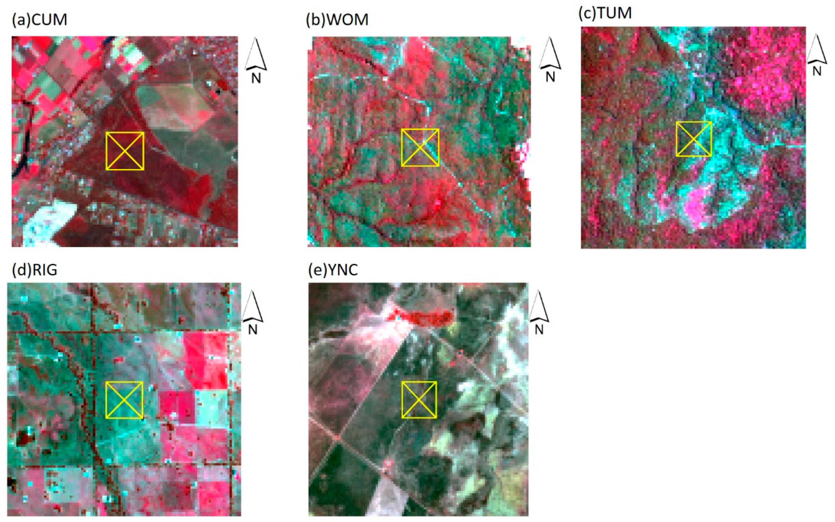
2.1. Field Sites

We selected five CO₂ flux sites in southeast Australia representing considerable variations in region, climate, and species, including three evergreen broadleaf forests (EBF) and two grassland (GRA) sites (

Table 1. Information on research sites. Climate types follow the Köppen classification system [54] (Cfa—warm temperate fully humid with hot summer, Cfb—warm temperate fully humid with warm summer, BSk—arid steppe cold). EBF and GRA in the vegetation type column represent evergreen broadleaf forest and grassland, respectively. ID—identifier; Jan—January; Oct—October; Lat—latitude; Lon—longitude; HLS—Harmonized Landsat and Sentinel-2 project.

Site ID	Full Name	CO2 Flux Years	Location (Lat, Lon)	Vegetation Type	Military Grid Reference System (HLS-Sentinel Tile)	Annual Precipitation (mm)	Climate Type	Reference
CUM	Cumberland Plain	Jan 2015–Oct 2018	−33.6152, 150.724	EBF	56HKH	800	Cfa	[55]
TUM	Tumbarumba	Jan 2015–Oct 2018	−35.6566, 148,152	EBF	55HFA	1000	Cfb	[56]
WOM	Wombat Forest	Jan 2015–Oct 2018	−37.4222, 144.094	EBF	55HBU	600	Cfb	[57]
RIG	Riggs Creek	Jan 2015–Jan 2017	−36.6499, 145.576	GRA	55HCV	650	Cfb	[58]
YNC	Yanco	Jan 2015–Oct 2018	−34.9893, 146.291	GRA	55HDB	465	BSk	[59]

, Figure 1).

The Cumberland Plain (CUM) site is located in a dry sclerophyll forest in the Hawkesbury Valley in central New South Wales. The canopy is dominated by Eucalyptus moluccana and Eucalyptus fibrosa.

The Tumbarumba (TUM) site is located in the Bago State Forest in southeastern New South Wales. The forest is classified as wet sclerophyll, and the dominant species is Eucalyptus delegatensis. The Wombat Forest (WOM) site is located in the Wombat State Forest, Victoria. The site is a secondary regrowth forest that was last harvested in 1980. The dominant tree species are Eucalyptus obliqua (messmate stringybark), Eucalyptus radiata (narrow leaf peppermint), and Eucalyptus rubida (candlebark), with an average canopy height of 25 m.

The Riggs Creek (RIG) site is located in the Goulburn–Broken catchment in northeastern Victoria, with the surrounding area dominated by broadacre farming practices. The vegetation cover is predominantly pasture. The Yanco (YNC) site is located within the Yanco region of New South Wales. The flux tower site in the Yanco area is located in the western plains of the Murrumbidgee catchment and is within a wider research area (60 × 60 km) that supports a network of OzFlux stations.

2.2. Data

2.2.1. Tower-Based Carbon Flux Data

All sites contained CO₂ flux data and incident photosynthetic active radiation (PAR_in) measurements during the research period. The carbon flux data at each site during the study period were collected by members of OZflux [60]. The CO₂ flux data at these sites were measured by an Li-7500 (Campbell Scientific Inc., MS, USA), which is an open-path infrared CO₂/H₂O gas analyzer, in half-hour time steps. These flux data were described in Beringer et al. 2011, 2017, Cleverly et al. 2016a, 2016b, and Li et al. 2017 [61,62,63,64,65]. Data were downloaded from the Australian Terrestrial Ecosystem Research Network (TERN) website (http://data.ozflux.org.au/portal/pub/listPubCollections.jspx) and then post-processed using the REddyProc tool [66]. The REddyProc tool was previously used to transform half-hourly CO₂ flux input data into half-hourly GPP data [67,68]. We used the daytime method, which avoids the CO₂ flux transfer uncertainties resulting from potentially problematic nighttime data [69]. This method was successfully used to evaluate the global carbon flux [1] to partition the CO₂ flux into GPP. Then, we aggregated the half-hourly GPP and PAR_in data on a daily scale. The aggregated flux tower-based GPP data are presented as GPP_EC in the following sections.

2.2.2. Sentinel-2 Remote-Sensing Products

We applied Sentinel-2 data from the Harmonized Landsat and Sentinel-2 (HLS) project to provide high-frequency multispectral data with moderate-to-high spatial resolution [70]. The HLS dataset provided remote-sensing reflectance with high spatial resolution that was atmospherically corrected, and the data were mapped to the Military Grid Reference System [71]. We used the HLS land surface reflectance product for Sentinel-2 data, which were resampled to 30-m spatial resolution from the HLS v4 dataset (Figure 1). We evaluated the effect of cloud cover on the satellite image by using the cloud and shadow masks provided in the HLS data.

2.2.3. MODIS GPP Product

This study also used the MOD17A2H GPP product as representative of light-use efficiency (LUE)-based GPP and compared it to the VI-based GPP estimation results. The MOD17A2H GPP product provided spatio-temporally continuous GPP data with 500-m spatial resolution for eight-day averages [2]. We chose the 3 × 3 pixels’ region around the flux tower from the MOD17A2H product, and the mean value of these pixels was set as the MODIS-based GPP result.

2.3. Methods

The main CO₂ flux footprint region is approximately 500 m around the flux tower [72,73], which is spatially representative of GPP_EC. The spatial resolution of the MOD17A2H product is 463 m. To compare the remote-sensing data, including Sentinel-2-based VI and MOD17A2H products, with tower-based CO₂ flux data at a fine scale, we selected the standard spatial window as 450 × 450 m around the flux tower, which was approximately 15 × 15 pixels of the Sentinel-2 data aggregated at 30-m spatial resolution.

2.3.1. Remote-Sensing-Based Indices

Eight VIs were calculated from the Sentinel-2 data, as shown in

Table 2. Vegetation indices derived from the Sentinel-2 multispectral instrument (MSI) sensor. The terms B2 to B8 are the abbreviations of band reflectance from the Sentinel-2 MSI sensor. The center wavelength of each band is as follows: B2 (490 nm), B3 (560 nm), B4 (665 nm), B5 (705 nm), B6 (740 nm), B7 (783 nm), B8 (842 nm). EVI—enhanced vegetation index; NDVI—normalized difference vegetation index; NIRv—near-infrared reflectance of terrestrial vegetation; CI—chlorophyll index; MTCI—medium- resolution imaging spectrometer (MERIS) terrestrial chlorophyll index; NDRE—normal deviation index of the red edge.

Index	Formulation	Reference
EVI	$\frac{2.5\times \left(B8-B4\right)}{B8+6\times B4-7.5\times B2+1}$	[74]
NDVI	$\frac{B8-B4}{B8+B4}$	[75]
NIRv	$\frac{B8-B4}{B8+B4}\times B8$	[76]
CI red edge (CIr)	$\frac{B7}{B5}-1$	[39,43]
CI green (CIg)	$\frac{B7}{B3}-1$	[39,43]
MTCI	$\frac{B6-B5}{B5-B4}$	[47]
NDRE1	$\frac{B6-B5}{B6+B5}$	[36]
NDRE2	$\frac{B8-B5}{B8+B5}$	[77]

. Three indices did not contain red-edge information, including the EVI [74], NDVI [75], and the near-infrared reflectance of terrestrial vegetation (NIRv [76]). Five of the indices, including one or more of the three Sentinel-2 red-edge bands (CIr, CIg, and MTCI) and two normal deviation indices of the red edge (NDRE1, NDRE2 [36,77]), were related to red-edge reflectance (band 5 to band 7 of the MSI sensor).

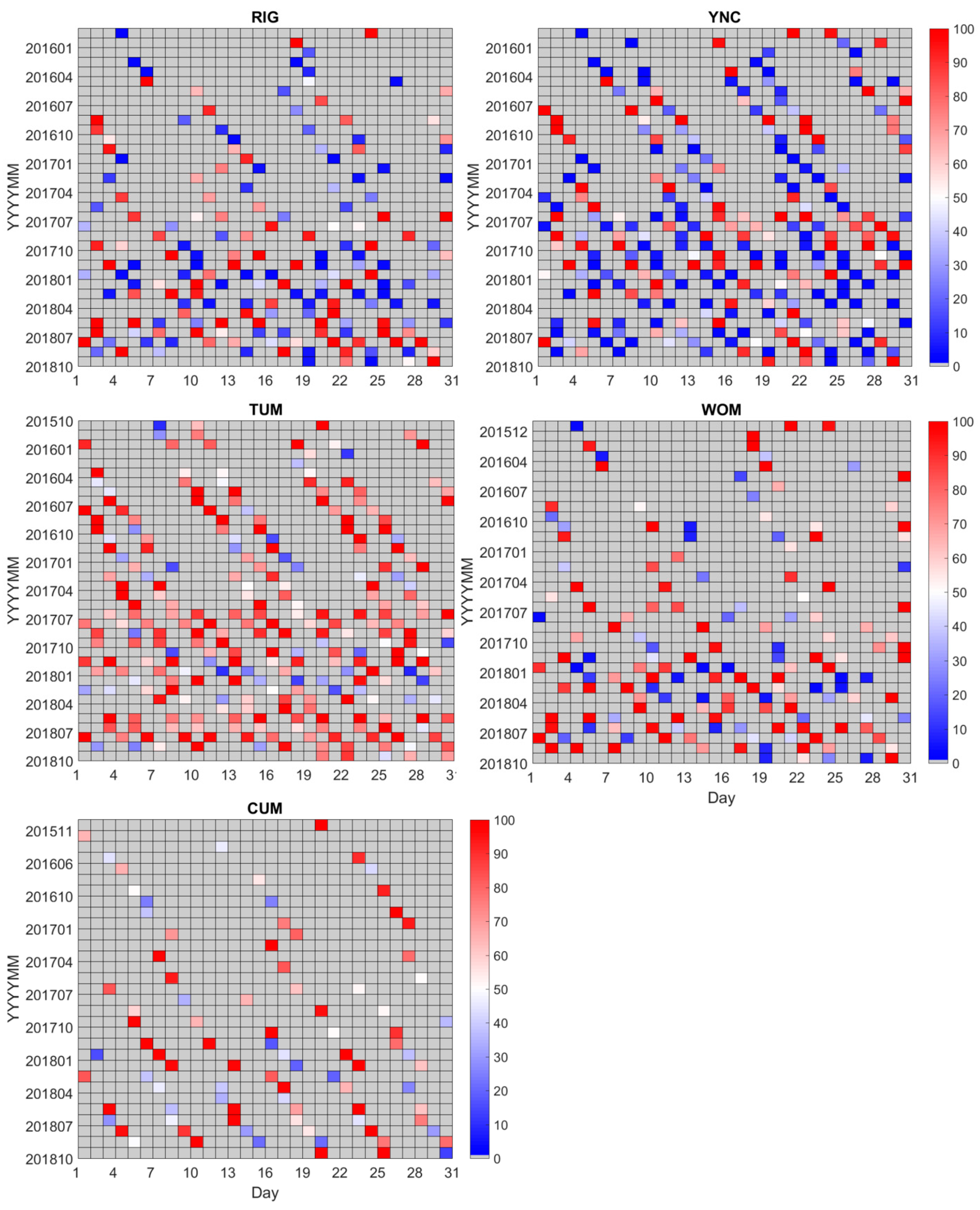
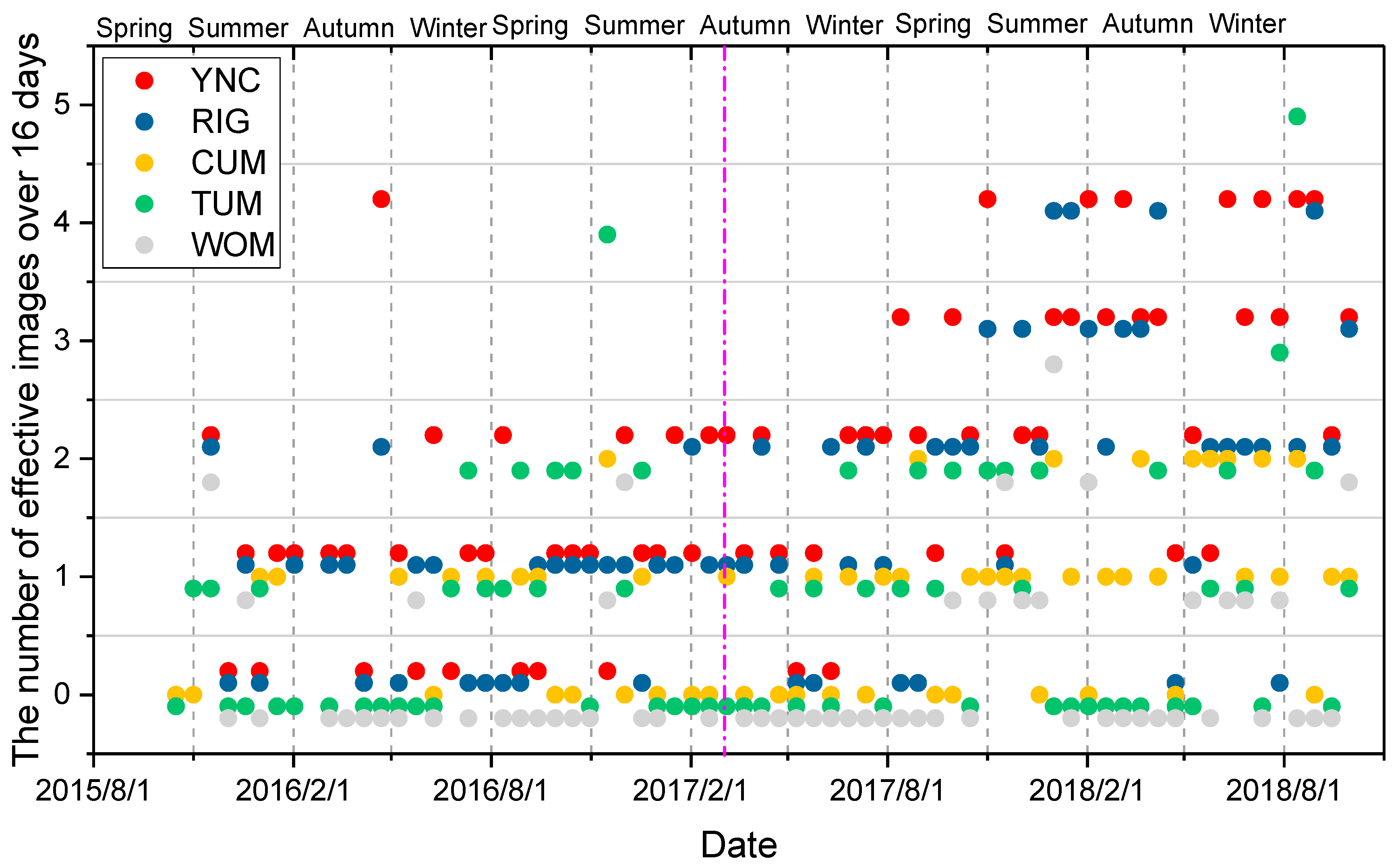
2.3.2. Evaluation of the Cloud Effect

For the Sentinel-2 data, the percentage of no cloud cover (Pclear) was defined as

$$P_{clear}=\frac{N_{clear}}{N_{clear}+N_{cloudcover}+N_{cloudshadow}},$$

(1)

where $N_{clear}$ is the number of pixels with no cloud cover, $N_{cloudcover}$ is the number of pixels with cloud cover, and $N_{cloudshadow}$ is the number of pixels with cloud shadow masks. Here, we defined the effective images as the data in the spatial image window with $P_{clear}$ values >0.7.

Cloud cover affects the diffuse scattering of light in the sky; thus, it changes the light intensity and influences the carbon assimilation rate for photosynthesis [78]. Here, we applied the concept of potential PAR ($PA{R}_{pot}$), which was the maximal incident PAR during the 16-day interval [79]. Therefore, the daily cloud effect at the site was defined as

$$\mathrm{CSI}=\frac{PA{R}_{in}}{PA{R}_{pot}}.$$

(2)

When the clear sky index (CSI) is approximately 1, clouds have little effect on the incident PAR.

2.3.3. Rebuilding the Time Series of Vegetation Indices at the Sites

The VIs were derived from the reflectance data that were affected by cloud cover, resulting in some temporal gaps. Thus, the rebuilding of the time series is important for filling the gaps resulting from missing VIs. We used the following steps to derive the spatio-temporally continuous VIs:

(1)

The reflectance was selected in each image from the Sentinel reflectance product in the 450 × 450-m spatial window.

(2)

The reflectance values were removed from the pixels where there were cloud and shadow masks.

(3)

The $P_{clear}$ was calculated in the spatial window.

(4)

The VI was calculated from the reflectance in each pixel where there were no cloud and shadow masks.

(5)

The maximal VI was chosen with P_clear > 0.8 during the standard interval in each pixel (here, we defined it as a 16-day interval from the first day of the year) as the true VI value [80].

(6)

A continuous VI time series in each pixel was rebuilt by a Savitzky–Golay filter [81].

The daily VI was interpolated from the rebuilt VI time series within a standard interval. Then, we selected the cloud-free images at the five sites during the peak of the growing season from 1 January 2016 to 1 October 2018, in order to characterize the spatial variance in vegetation in the study area. The standard deviations of CIr and EVI in the spatial window were used to quantify the spatial heterogeneity of the total canopy chlorophyll content.

2.3.4. Estimating GPP by VI and Statistical Analysis

Our hypothesis is that GPP is a function of the VI and PAR_in, as shown below.

$$\mathrm{GPP}\propto \mathrm{VI}\times {\mathrm{PAR}}_{in}.$$

(3)

Because different remote-sensing chlorophyll-related VIs have unique ranges and the environment has various conditions, the relationship for the VI_i–PAR_in–GPP model was not constant.

$${\mathrm{GPP}}_{V{I}_i}=a_i\times {\mathrm{VI}}_i\times {\mathrm{PAR}}_{in}+b_i.$$

(4)

In Equation (4), the coefficient values of a_i and b_i were changed according to the specific VI_i. In each iteration, we randomly selected 70% of the observations (calibration set), including 16-day interval data of the mean GPP_EC, time-series rebuilt VI_i, and mean PAR_in, to calibrate the coefficients a_i and b_i. The remaining 30% (validation set) of the observations were used to validate the relationship between GPP_VIi and GPP_EC. The correlations of GPP_VIi and GPP_EC in the validation set were described by the determination coefficient (R²), root-mean-square error (RMSE), and related RMSE (rRMSE, which is defined as the ratio of RMSE and mean observed GPP). We then repeated this iteration 100 times. The mean R², RMSE, and rRMSE values of the 100 iterations in the validation set were used to quantify the temporal relationship between GPP_VIi and GPP_EC, while the mean a_i and b_i values in the calibration set were the general coefficients of VI_i–PAR_in–GPP.

Then, we mapped the GPP distribution based on the spatio-temporally continuous VI_i and the relationship of VI_i–PAR_in–GPP at each site. We simplified the expression for the relationship of VI_i–PAR_in–GPP into GPP_VI; for example, GPP_EVI represents the GPP estimated by EVI and PAR_in in the later sections.

3. Results

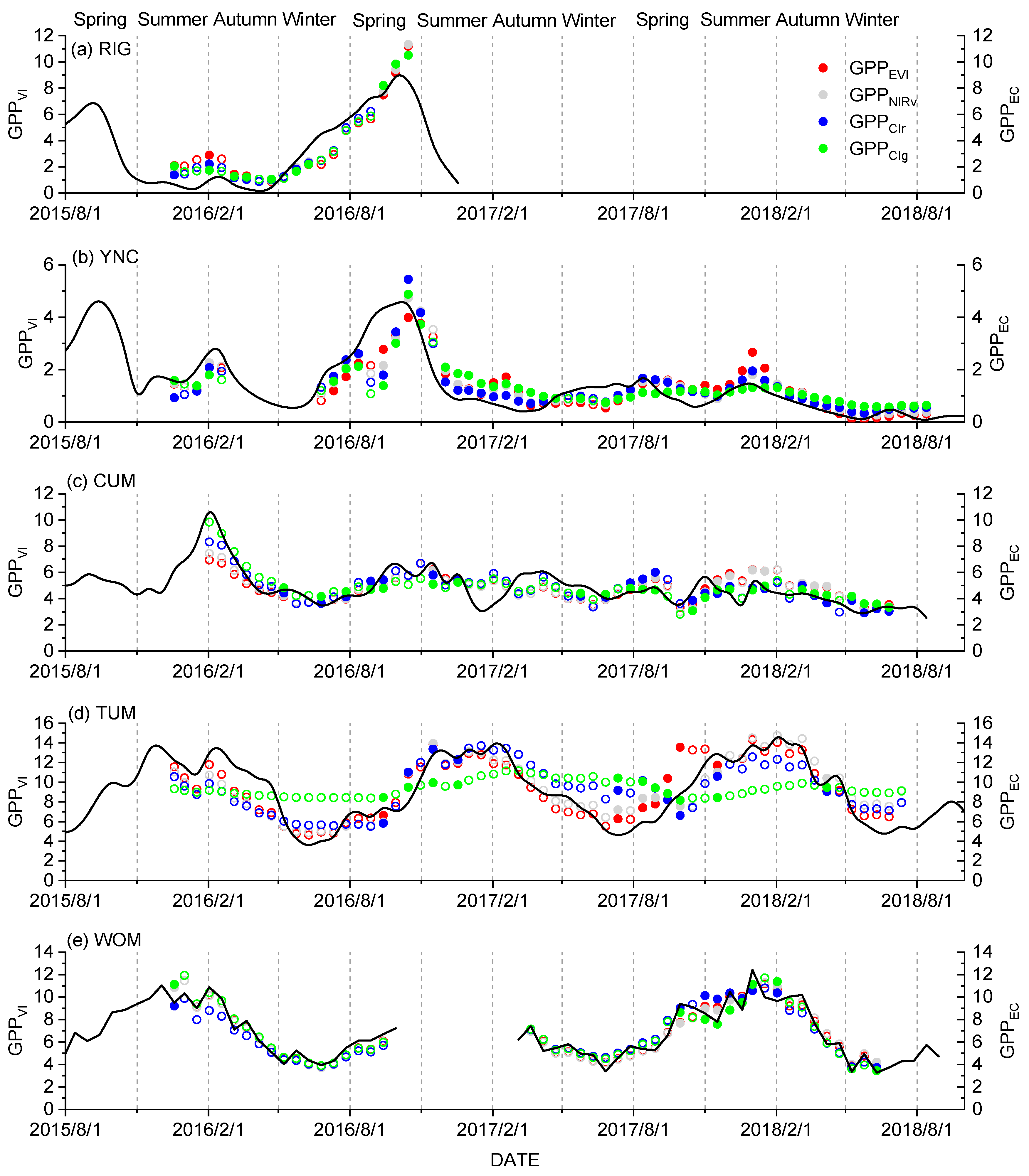
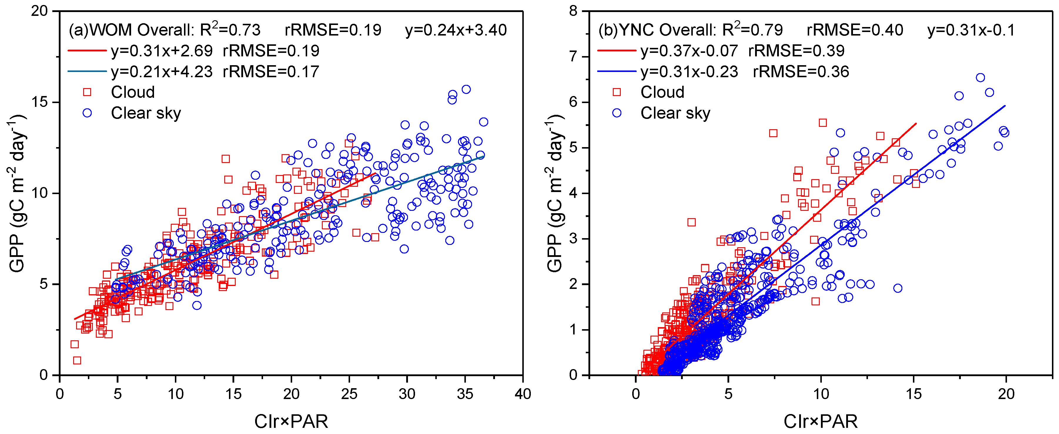
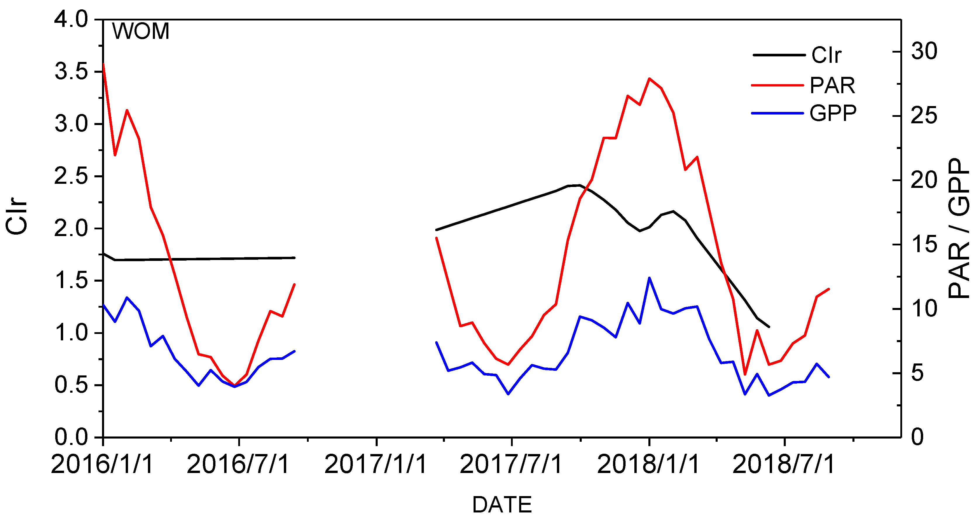
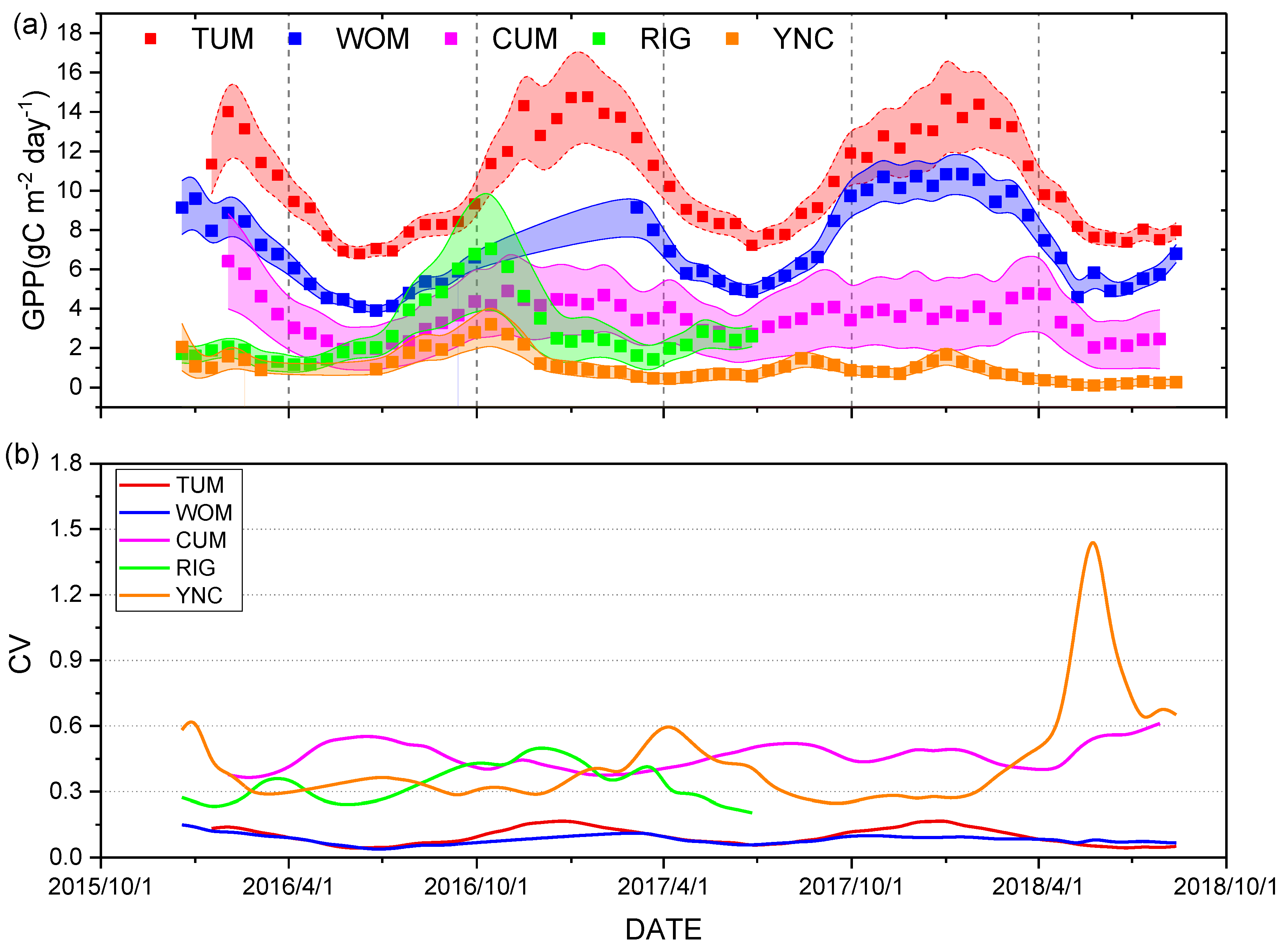
3.1. Temporal Relationship between GPP_VI and GPP_EC

Cloud cover affected the number of effective images of the sites, determining whether the gaps in the VI needed to be filled or not. The percentage of cloud-free pixels in the Sentinel-2 tiles of grassland sites was mostly less than 50%. In particular, at YNC, more than 70% of the data had $P_{clear}$ values greater than 30%. However, the EBF sites contained much more cloud cover than did the GRA sites. At the TUM site, 10% of the data had less than 70% cloud cover (Figure 2). During the 16-day standard interval, the number of effective images was less than two at the grassland sites before the launch of Sentinel-2A (Figure 3). After the launch of Sentinel-2B, the networking system of Sentinel-2A and Sentinel-2B increased the number of effective images to four during the 16-day interval. The number of effective images at CUM also significantly increased (average from one image per month to two or more per month). During the end of winter to the early summer, the number of effective images after Sentinel-2B launched was two times more than when the images were obtained by Sentinel-2A alone. However, during the end of summer and early autumn at the TUM and WOM sites, there were almost no cloud-free images due to the rainy season in southeast Australia. Thus, although the networking Sentinel-2 system has a five-day revisit cycle, it cannot get low-cloud-cover images during continuously rainy days at the sites with humid summers.

The general relationships between red-edge- and non-red-edge-related VIs derived from Sentinel-2 with GPP_EC in the main footprint region of the flux towers at the EBF sites are shown in

Table 3. The algorithm results for 16-day average daytime gross primary productivity (GPP) estimated at evergreen broadleaf forest (EBF) sites, with the determination coefficient (R²), root-mean-square error (RMSE; unit in gC∙m⁻²∙day⁻¹), and relative RMSE (rRMSE) presented. We employed the equation GPP_EC = a × VI × PAR + b here, where the vegetation index (VI) is the rebuilt time series, and PAR is the photosynthetic active radiation. The number of samples at each site is presented in parentheses after the site name. The numbers in bold represent the highest R², lowest RMSE, and lowest rRMSE values.

	TUM (N = 60)					WOM (N = 36)					CUM (N = 56)
	R2	RMSE	rRMSE	a	b	R2	RMSE	rRMSE	a	b	R2	RMSE	rRMSE	a	b
CIr	0.53	2.35	0.25	0.36	5.01	0.87	0.96	0.14	0.30	2.88	0.53	1.05	0.21	0.31	−0.13
CIg	0.08	3.33	0.35	0.01	8.32	0.90	0.78	0.11	0.04	2.75	0.53	1.01	0.21	0.04	1.90
MTCI	0.75	1.70	0.18	0.32	2.89	0.83	0.98	0.14	0.21	2.47	0.36	1.25	0.25	0.18	0.47
NDRE1	0.73	1.77	0.19	0.36	3.28	0.89	0.82	0.12	0.24	2.58	0.45	1.15	0.23	0.21	0.60
NDRE2	0.70	1.86	0.20	0.29	3.52	0.87	0.86	0.12	0.19	2.65	0.46	1.14	0.23	0.18	0.42
EVI	0.76	1.67	0.18	2.48	2.83	0.91	0.74	0.11	1.85	2.54	0.38	1.23	0.25	1.15	1.85
NIRv	0.70	1.89	0.20	5.40	3.67	0.91	0.75	0.11	4.17	2.52	0.43	1.17	0.24	2.92	1.59
NDVI	0.69	1.92	0.20	1.06	4.26	0.90	0.78	0.11	0.81	2.60	0.38	1.23	0.25	0.58	1.46
MOD17A2H	0.66	1.76	0.30	-	-	0.85	0.93	0.18	-	-	0.28	0.97	0.28	-	-

. These results show how much of the temporal variation in GPP_EC can be captured by GPP_VI. Both red-edge VIs and non-red-edge VIs corresponded closely to GPP_EC during the study period at the WOM and TUM sites. The WOM site showed the highest correlation between GPP_VI and GPP_EC across all VIs. The non-red-edge VIs, such as EVI and NIRv, explained more than 90% of the temporal variance in GPP, with an average rRMSE of approximately 11%. The red-edge-based GPP_VI, including CIr, CIg, MTCI, NDRE1, and NDRE2, showed R² values of 0.87, 0.90, 0.83, 0.89, and 0.89 with GPP_EC, respectively. The TUM site also showed similar results, while the highest correlation between GPP_VI and GPP_EC in the red-edge VIs was found for MTCI (R² = 0.75, rRMSE = 0.18). The other red-edge VIs showed R² values of 0.73, 0.70, 0.53, and 0.09 for NDRE1, NDRE2, CIr, and CIg with GPP_EC, respectively. The non-red-edge-related VIs showed high relevance with GPP_EC (average R² = 0.73, rRMSE = 0.19). The CUM site showed a different result between the red-edge and non-red-edge VIs with GPP_EC. The GPP_CIr and GPP_CIg corresponded well with GPP_EC, with an average R² of 0.56. However, other red-edge-related VIs (NDRE1, NDRE2, MTCI) showed low correlation with GPP_EC. The non-red-edge VIs, including EVI, NDVI, and NIRv, showed R² values of 0.38, 0.43, and 0.38 with GPP_EC, respectively.

Table 4. The algorithm results for the 16-day average daytime GPP estimated at grassland (GRA) sites, with the determination coefficient (R²), RMSE (unit in gC∙m⁻²∙day⁻¹), and rRMSE presented. We adopted the equation GPP_EC = a × VI × PAR + b here, where the VI is the rebuilt time series, and PAR is the photosynthetic active radiation. The number of samples at each site is presented in parentheses after the site name. The first two series of results are based on rebuilt VIs in a 16-day standard interval. The series YNC (N = 109) is based on rebuilt VIs in eight-day standard intervals. The numbers in bold represent the highest R², lowest RMSE, and lowest rRMSE values.

	RIG (N = 17)					YNC (N = 54)					YNC (N = 109)
	R2	RMSE	rRMSE	a	b	R2	RMSE	rRMSE	a	b	R2	RMSE	rRMSE	a	b
CIr	0.87	1.02	0.37	0.32	0.14	0.69	0.63	0.46	0.31	−0.05	0.89	0.34	0.33	0.31	−0.29
CIg	0.84	1.13	0.42	0.04	0.37	0.48	0.80	0.59	0.03	0.32	0.73	0.53	0.51	0.03	0.00
MTCI	0.54	2.05	0.76	0.32	−1.23	0.08	1.10	0.81	0.02	1.04	0.12	0.95	0.93	0.11	1.80
NDRE1	0.51	2.08	0.79	0.27	−0.79	0.23	0.99	0.73	0.10	0.03	0.37	0.80	0.78	0.12	−0.60
NDRE2	0.55	1.99	0.76	0.23	−0.73	0.25	0.98	0.72	0.10	−0.01	0.41	0.78	0.76	0.11	−0.66
EVI	0.77	1.36	0.52	1.60	−0.87	0.61	0.69	0.51	0.97	−0.32	0.76	0.50	0.49	0.99	−0.53
NIRv	0.86	1.07	0.39	2.77	−0.25	0.66	0.64	0.47	2.30	−0.13	0.83	0.42	0.41	2.32	−0.34
NDVI	0.66	1.67	0.65	1.31	−1.47	0.49	0.80	0.59	0.49	−0.10	0.76	0.50	0.49	0.52	−0.48
MOD17A2H	0.66	1.76	0.30	-	-	0.81	0.91	0.17	-	-	0.85	0.93	0.18	-	-

shows the temporal relationship between different GPP_VI and GPP_EC at the grassland sites. At RIG, the red-edge VI-related GPP_CIr and GPP_CIg had R² values of 0.87 and 0.84 with GPP_EC, respectively, whereas the non-red-edge VI-related GPP_NIRv and GPP_EVI also showed high R² values of 0.86 and 0.77 with GPP_EC, respectively. The results at the YNC site were similar to the results at the RIG site. The GPP_CIr correlated closely with GPP_EC (average R² = 0.69), but other red-edge-related GPP_VI corresponded poorly to GPP_EC. The GPP_EVI and GPP_NIRv showed R² values of 0.61 and 0.66 with GPP_EC, respectively.

Both non-red-edge-related GPP_EVI and red-edge-related GPP_CIr showed robust correspondence with the GPP_EC across all sites, with an average R² > 0.70 and RMSE < 1.5 gC∙m⁻²∙day⁻¹. The red-edge-based GPP_CIr coupled with PAR showed high correspondence with GPP at the GRA sites. The highest correlation with GPP_EC was observed in CIr × PAR, with an average R² greater than 0.75 and rRMSE less than 0.39 (Table 4). The relationship between GPP_CIr and GPP_EC had rRMSE values that were 0.15 and 0.05 lower than those for GPP_EVI at RIG and YNC, respectively. At some EBF sites, EVI × PAR had low rRMSE values with GPP_EC compared with the other red-edge-based VIs. At TUM and WOM, GPP_EVI had a lower uncertainty than GPP_EC, with an average RMSE of 1.42 gC∙m⁻²∙day⁻¹ and an rRMSE that was 0.03 less than that for GPP_CIr. However, the red-edge-based VIs, including CIr and CIg, coupled with PAR_in, had lower RMSE values than the other VI-based models at CUM (Table 3).

The red-edge-related GPP_CIr and GPP_CIg and the non-red-edge-related GPP_EVI and GPP_NIRv corresponded well with GPP_EC at all sites. Figure 4 shows the time-series relationship between GPP_VI and GPP_EC during the study period. These four VIs showed similar trends with GPP_EC from November 2015 to November 2016 at RIG. When the GPP_EC was high in the summer, the GPP_VI showed a robust relationship with GPP_EC in these four VIs at YNC. There were fewer effective images obtained at the EBF sites than at the GRA sites; thus, the GPP_VI did not track the GPP_EC variance. From January 2017 to April 2017, there were little available data for VI retrieval, and all GPP_VI had different trends with GPP_EC at CUM. The GPP_CIg showed limited variance at TUM; thus, it exhibited a high bias with GPP_EC during the study period. At WOM, all of the GPP_VI corresponded with GPP_EC across the different seasons.

The Sentinel-2-based red-edge VIs such as CIr exhibited similar estimating accuracy with GPP_EC under gap-filled days and non-gap-filled days (Figure 5). At WOM, the rRMSE under a cloudy sky was 0.19, which was similar to the rRMSE under a clear sky (0.17). A similar result was also observed at the YNC site. However, the correlation coefficients a and b were different for cloudy and clear days at WOM and YNC. The seasonal change in CIr in WOM was not significant, and the GPP change was mostly accompanied by a change in PAR_in (Figure 6). High cloud cover led to a low clear sky index (CSI), which influenced the image quality; thus, the gaps in the VIs in these periods needed to be filled (Figure 4). With the VIs rebuilt on a daily scale, the relationship between GPP_EC and GPP_CIr was different between clear and cloudy days; thus, more available data are required to investigate the relationship between the time series rebuilt in the red-edge index and GPP_EC.

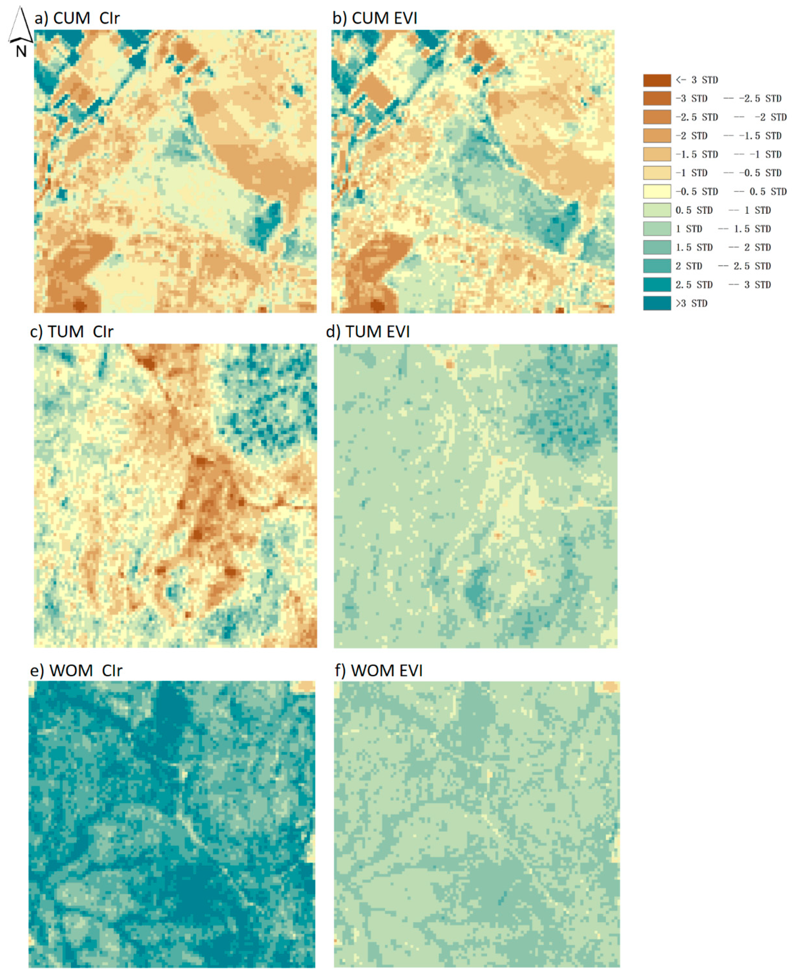
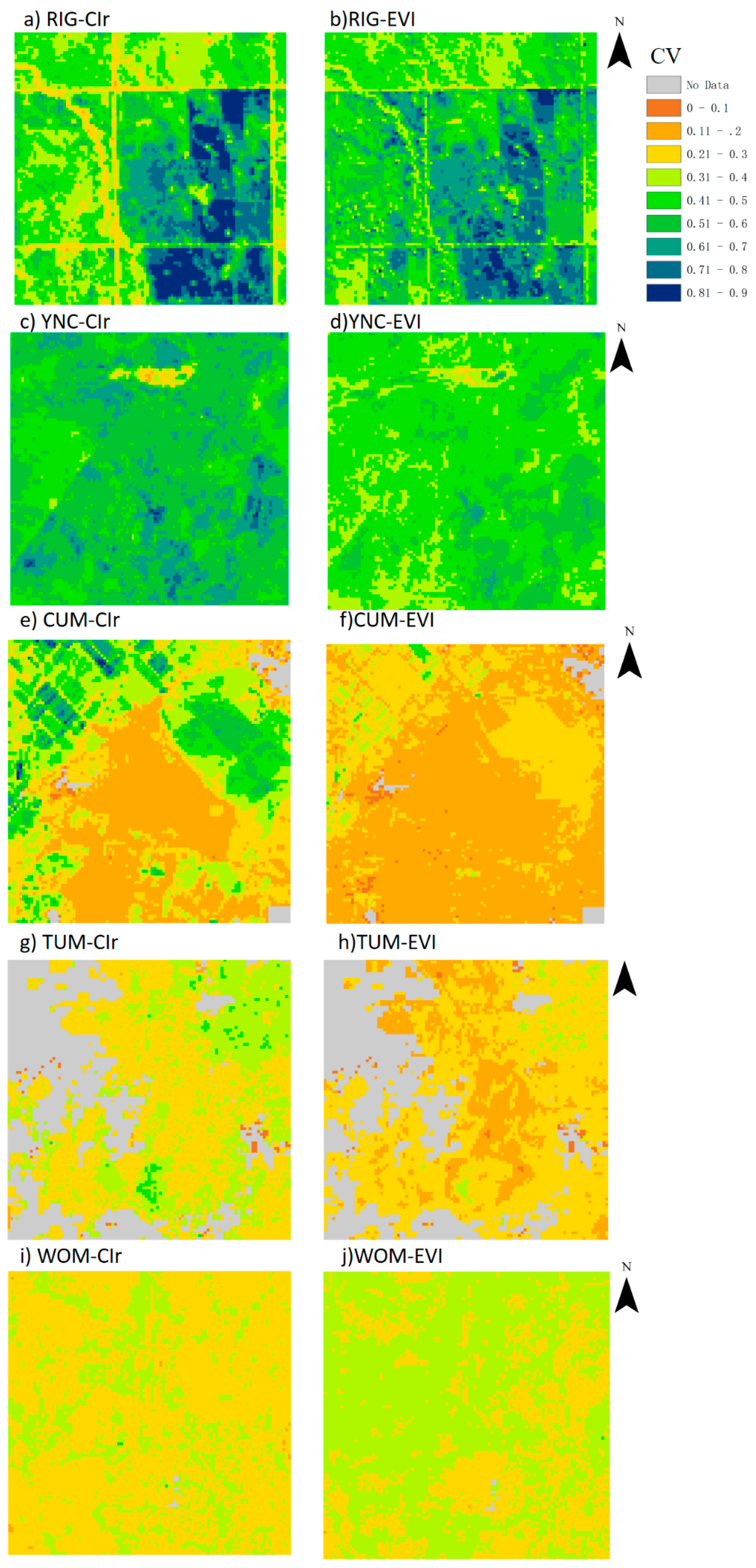
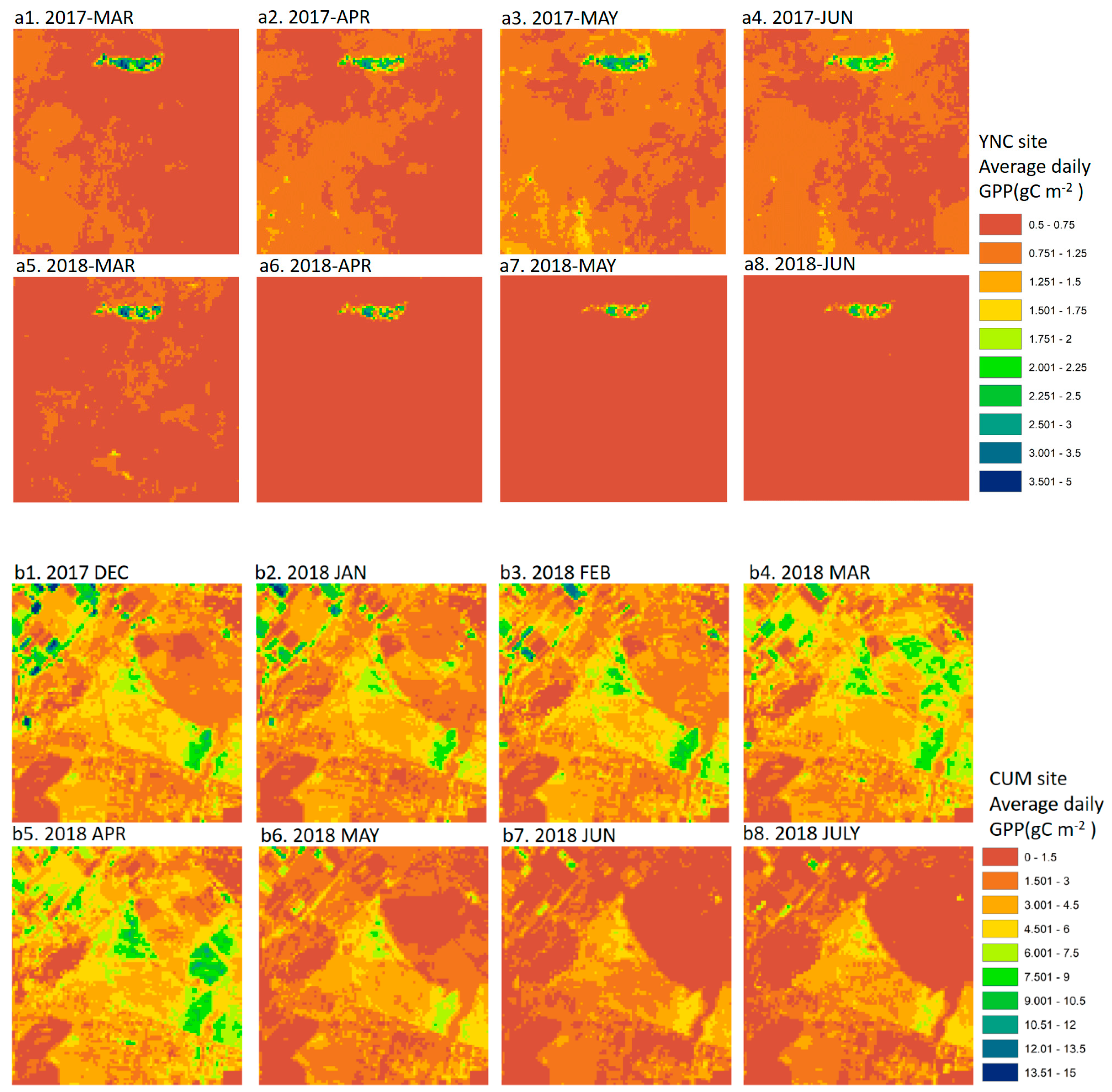
3.2. Spatial Distribution of GPPCIr

We used 30-m resampled Sentinel-2 data to quantify the spatial distribution of non-red-edge VIs and red-edge VIs (Figure 7). The coefficient of variance (CV) values of the red-edge CI in the EBF sites in January 2018 were 0.56, 0.16, and 0.14 for CUM, TUM, and WOM, respectively. The CVs of the EVIs near each site were 0.40, 0.12, and 0.08 for CUM, TUM, and WOM, respectively. In the forest sites, the CV of the red-edge-based CIr exhibited a higher spatial difference than the non-red-edge-based EVIs. The spatial variance in CIr was higher in the natural forest of TUM than at WOM. The CIr showed 11 value levels; however, the EVI showed concentrated values between −2 standard deviations (STDs) and 2 STDs, whereas the artificial forests, such as those at the WOM site, were more homogeneous than the natural forests and still showed eight major levels of CIr values compared with the five levels in the EVI. The spatial heterogeneity at the CUM site showed large differences in CIr around the center of the image, but it showed a similar range of EVI around the site.

We mapped the range of GPP at five 3 × 3-km sites based on their CIr × PAR–GPP relationship, as shown in Table 3 and Table 4. The GPP exhibited higher seasonal variance at the GRA sites than at the EBF sites. Figure 8 shows the annual GPP variance at these sites. The central footprint of CUM was forest, while the other parts were grassland, croplands, and artificial land cover (Figure 1). The forest component showed low intra-annual variance (CV < 0.2) throughout the year, whereas the grass component showed high intra-annual GPP variance (CV > 0.4). The other two forest sites were mostly covered by the EBF, showing CV ranges of 0.2 to 0.4 and 0 to 0.4 for WOM and TUM, respectively. For the grassland sites, the RIG site showed an annual GPP with a CV range from 0.3 to 0.8, and the YNC showed a CV range from 0.4 to 0.8. The land-cover reference image from Google Earth was used for comparison, as shown in Figure 1, which showed that the annual GPP variance in grassland and croplands was much higher than that in the EBFs.

The spatial variance in GPP differed among the different seasons. Figure 9a shows the GPP differences on different dates. The GPP showed high variance at the forest sites (TUM, WOM). During the peak of the growing season (December to January), each site showed higher GPP variance than that in the winter (July). Unlike the standard deviation, which was high at the peak of the growing season, the GPP showed less spatial variance at the TUM and WOM forest sites than at the other sites, with CV values less than 0.15 in all seasons (Figure 9b). CUM, which had two major types of vegetation cover, always showed high spatial variance in GPP (CV = 0.5) in different periods. The spatial variance always showed a CV value of 0.3 at the GRA sites.

The CUM site is a heterogeneous site with three major types of vegetation. Each vegetation type showed a different growing condition across seasons. Each vegetation type had different growth trends of GPP (Figure 10). Thus, the GPP STD at the 3 × 3-km footprint region was always high at the CUM site and it showed a wide boundary of GPP during the study period (Figure 9). The high STD of YNC in 2018 was because, in 2018, most of the vegetation showed a low value near the flux tower except the north portion of the 3 × 3-km footprint region with forest cover. From April 2018 to June 2018, the GPP was greater than 1.75 in the north part of the footprint region, with other areas having GPP values less than 0.75. However, the GPP in 2017 was approximately 1 in all areas except the forests. Thus, the STD showed a high value in 2018.

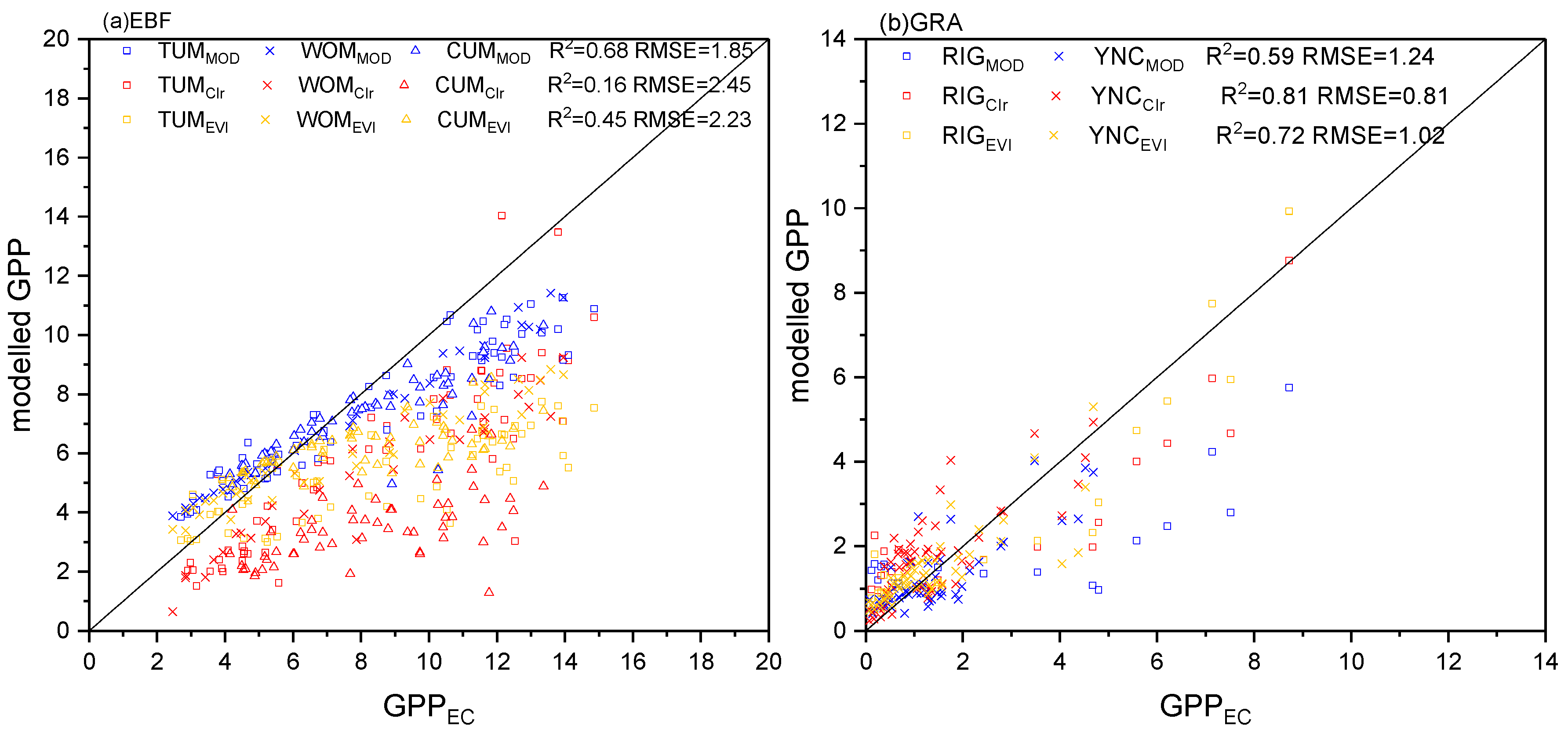
3.3. Comparison of GPP Modeling Results based on Sentinel-2 Data and MODIS Products

We compared our GPP_VI with an LUE-based GPP product (MOD17A2H) in the footprints near the flux tower sites. Table 3 shows that GPP_EVI exhibited a higher correlation with GPP_EC than MOD17A2H at the EBF sites. Table 4 shows that the red-edge-based GPP_CIr had a lower rRMSE value of 0.07 with GPP_EC than that of the MODIS product at the GRA sites. The non-red-edge GPP_EVI based on the coefficients at each site had a higher correlation with GPP_EC than did the MOD17A2H product. Both GPP_CIr and GPP_EVI showed a higher correlation than MOD17A2H with GPP_EC at the spatially heterogeneous CUM sites. However, at the sites with homogeneous vegetation distribution near the flux tower footprint region such as WOM and YNC (Figure 8), the estimation accuracy between MOD17A2H and GPP_EC was similar to that for GPP_VI and GPP_EC (Table 3 and Table 4).

To evaluate the effectiveness for large-scale GPP estimation, we used the same series of coefficients for estimating GPP across different sites (Figure 11). Figure 11 shows that the Sentinel-2 red-edge-based GPP_CIr corresponded better to GPP_EC than GPP_EVI and MOD17A2H in grasslands, with the highest R² and RMSE values as 0.2 gC∙m⁻²∙day⁻¹ less than those obtained using other methods. At the EBF sites, MOD17A2H showed the highest R² and the lowest RMSE. Unlike the similar coefficient values of a and b at the GRA sites, the key coefficient b in GPP_CIr exhibited large differences across the three EBF sites (5.01, 2.88, and −0.13 for TUM, WOM, and CUM, respectively, Table 3). In addition, the key coefficient a in GPP_EVI exhibited large differences across the three EBF sites (2.48, 1.85, and 1.15 for TUM, WOM, and CUM, respectively, Table 3), which led to high systemic bias with GPP_EC.

4. Discussion

4.1. Improvements to GPP Modeling with Vegetation Red-Edge Information

Previous research confirmed that total canopy chlorophyll content and incident photosynthetic active radiation (PAR_in) are key drivers of GPP in many croplands [39,45,46]. Our results compared the relationships between VIs × PAR_in and GPP_EC in grasslands and EBF sites, where the VIs were derived with and without red-edge bands. The results of this study showed that red-edge-based VIs such as CIr and CIg coupled with PAR have a higher correlation with GPP_EC than other VIs without red-edge information in GRA sites, which is similar to the results of previous research [48]. The red edge contains information on vegetation conditions and is sensitive to changes in chlorophyll; thus, red-edge-based VIs, such as CIr, can track the seasonal changes in the chlorophyll pigment pool [37,52,82]. The vegetation pigment pool plays an important role in long- or medium-term GPP estimations [36]; thus, red-edge VIs can significantly explain the temporal variance in GPP in cropland and grassland sites [39,52,83].

Furthermore, this study also tested the relationship between CIr × PAR_in and GPP_EC in the forest sites. However, GPP_EVI was more representative of GPP_EC than GPP derived from the red edge in the EBF sites, which was also shown in previous studies [48]. There was a small rRMSE difference between GPP_CIr and GPP_EVI. This result indicated that GPP_CIr could partly evaluate the variance in GPP in EBF sites. On the one hand, at WOM sites, as in EBF sites, the seasonal change in CIr was not significant (Figure 6). The total GPP was more limited by the incident PAR but not the CIr-related chlorophyll content; thus, under clear and cloudy conditions, the major limitation to GPP is only PAR. Research showed that the reflectance chlorophyll/carotenoid index is more sensitive to intra-annual changes in the pigment pool at evergreen sites [38]; thus, the red-edge-based VIs cannot track the seasonal changes in the pigment pool. Conversely, the light-use efficiency at evergreen forest sites is mostly controlled by water and PAR_in; thus, the seasonal changes in the chlorophyll content did not lead to significant stress and photosynthesis decline [84]. In addition, the VI × PAR_in-based GPP model represented the medium condition of monthly scale GPP that cannot fully catch the highest and lowest GPP values [23]. The accurate GPP value over a shorter time period should also consider the short-term changes in weather conditions. Thus, the LUE-based models considering short-term weather situations such as MODIS GPP exhibited better performance with GPP_EC than other GPP_VI [85,86]. For cross-site studies in evergreen forests, a previous study also showed that the MODIS GPP exhibited better performance than the GPP estimated by the red-edge index [48]. The MTCI was based on the MERIS with a different central wavelength for band 8 in Sentinel-2 MSI (740 nm) and MERIS band 10 (753 nm). Additionally, the MTCI explained less than 40% of the carbon flux well in grasslands and evergreen forests [48]. Thus, the MTCI showed a low R² and high RMSE in these sites (Table 3 and Table 4). To summarize, the GPP estimation by VI in evergreen forests needs to consider vegetation growing stress such as seasonal pigment changes [38,87] and light conditions [88,89].

4.2. Advantages of Sentinel-2 High-Spatial-Resolution Data for GPP Modeling

The Sentinel-2 network provided data with a higher revisit period (less than five days) than the Landsat data (16 days), and it also contained a sensor with 20-m spatial resolution (resampled to 30-m spatial resolution in this study). The high-spatial-resolution data provided more detailed information on the physiological variance in vegetation. Figure 7 shows that the CIr value was much higher in forestland than in grassland, which indicated that the canopy chlorophyll content in the forest was higher than that in grassland. The maximal CIr value was found to the north of the tower at the YNC site, which is a tree-covered area with a CIr value that was 1.6 times higher than that in the other grassland area (Figure 7e). Additionally, CIr can precisely describe the physiological conditions and seasonal changes in vegetation; thus, it is suitable for high-spatial-resolution GPP mapping (Figure 8 and Figure 9). The reason for the high CV at grass sites was the trees in the 3 × 3-km range near the central towers of RIG and YNC. On the other hand, the GPP_EVI and GPP_CIr at CUM, which is spatially heterogeneous, corresponded better to GPP_EC than to the MOD17A2H product. Furthermore, the high spatial resolution of GPP_CIr also indicated the high spatial variance in seasonal changes in GPP at the CUM site, because grass and forest vegetation have different growing speeds and different GPP conditions. This result indicated that the high-spatial-resolution Sentinel-2 data were suitable for characterizing the intra-annual spatial changes in GPP variance. Conversely, at the sites where there was more homogeneous land-cover type, such as the WOM and YNC sites, the relationships between GPP_MOD and GPP_EC, GPP_CIr, and GPP_EC were similar. With a single type of vegetation near the flux tower, the vegetation growing had a similar trend under the same environment and nutrient conditions; thus, the spatial resolution of the VI input did not affect the GPP estimation accuracy.

The networking systems of Sentinel-2A and B have a higher revisit period than the 16-day Landsat data, which enhanced the tracking ability of mid-term or long-term GPP variance. At the YNC grassland site, which is a dry area with few cloudy days, Sentinel-2 provided data with an average revisit period of three days. After the launch of Sentinel-2B, the YNC site had almost no missing data at the 16-day interval (Figure 2 and Figure 3). Because there was greater availability of cloud-free data at this site, the spatio-temporally continuous VIs also exhibited good performance at the eight-day standard interval. Under these circumstances, the correlation between VI × PAR and GPP_EC was much higher than that modeled at the 16-day standard interval. At the YNC site, the R² between CIr and GPP increased from 0.67 to 0.89, whereas the rRMSE decreased by 11% (Table 4). This result suggested that, with the greater number of effective images obtained by Sentinel-2, GPP_VI was more representative of GPP_EC because VIs can capture the mid-term changes in the vegetation pigment pool. The launch of Sentinel-2B increased the revisit period of the Sentinel-2 network, providing more effective data during spring and summer for the EBF sites. There were at least two effective images for all seasons except autumn at the EBF sites. However, although Sentinel-2B shortened the revisit period, the data were still less effective at the 16-day standard interval during the autumn. There was only one effective image at the WOM site and two at the TUM site during the autumn of 2018. Although the networking Sentinel-2 system had a five-day revisit period, with more cloudy days during the peak of growing season in some humid climate types, there were limited observations when they had the highest ecosystem GPP value. Thus, it limited the effectiveness of VI values to capture the magnitude of GPP_EC.

4.3. Outlook for High-Spatial-Resolution Satellite GPP Mapping

Our results demonstrated that the high-spatial-resolution and multi-temporal Sentinel-2 red-edge data corresponded well with GPP_EC. The red-edge-based vegetation index CIr coupled with PAR showed less bias with GPP_EC than the other VIs at all sites. We successfully mapped the spatio-temporally continuous GPP near the footprint region at each site based on the local relationship of red-edge VIs and GPP_EC.

Cloud cover affected the correlation between GPP and VIs (Figure 5). We selected CIr as an example to evaluate the relationship between GPP and VI. With the VI rebuilt on a daily scale, the correlation between GPP and VI × PAR is similar under clear sky and cloudy days. Although the rRMSE of the daily GPP estimation at WOM was low, the rRMSE of CIr was lower on clear sky days than on cloudy days. The YNC site showed similar results, with an rRMSE reduced by 0.04 on clear days compared with the overall rRMSE. However, the key coefficients of a and b in the relationship of CIr–PAR_in–GPP had 20–50% difference under gap-filled CIr-based GPP and non-gap-filled values. On the one hand, cloud cover change affects the amount of PAR_in, which leads to bias in GPP estimates. Shaded leaves and sunlit leaves received different amounts of PAR_in under different sky conditions, and they had different LUEs in the same tree; thus, the relationship of VI–PAR_in–GPP differed under clear sky and cloudy conditions [90]. Therefore, the tower-based spectra measurement under different levels of PAR_in could help determine the calibration coefficients a and b for the relationship between VI and GPP [91,92,93,94]. However, because the optical remote-sensing method cannot obtain effective images under cloudy conditions, the representativeness of the rebuilt VI time series depends on the effective VI that appears in the standard interval.

There are two possible ways to improve the performance of GPP_VI for capturing the seasonal and shorter temporal trend. One on hand, in order to get more effective satellite-based data during the cloudy conditions, one can apply multi-source remote-sensing data to improve the VI quality for rebuilding the time series VI during the peak of growing season [95]. The amounts of high-spatial-resolution remote-sensing data are increasing, such as Landsat-8 Operational Land Imager (OLI) and Chinese GF Wide-Field Camera (WMV), whereby the combination of these sensors can both improve the spatial resolution and revisit period [96]. This increase in data benefits the GPP mapping ability on a regional and continental scale. One the other hand, the chlorophyll-related VIs (such as CIr and EVI) are more related to the seasonal change of GPP, but not the short-term change [52]. Therefore, further research can apply some red-edge-related VIs for detect the seasonal change of chlorophyll content and couple the weather condition stress and chlorophyll fluorescence to capture short-term GPP variance [97,98].

For regional- or continental-scale mapping, a series of stable values for coefficients a and b is important. Similar coefficients of a and b in the CIr–PAR_in–GPP relationship were shown at the YNC and RIG sites. Thus, a cross-site comparison with one set of coefficients for GPP_CIr showed high correlation and low uncertainties with GPP_EC at the two grassland sites (Figure 11b). This result suggested that GPP_CIr could be used to map GPP at a large scale. However, the modeled GPP showed significant systematic bias compared with GPP_EC because, at each forest type, the relationship between GPP_VI and GPP_EC was not a constant value across these sites. These data showed that high uncertainties occurred if one set of coefficients was used to estimate GPP with GPP_CIr across the EBF sites (Figure 11a). There were several reasons for this result. The canopy chlorophyll content changes slowly at the EBF sites [99]. Unlike EVI, which changes slowly during the growing season, CIr is highly affected by the canopy chlorophyll content and the amount of available data. Therefore, during the rainy season, the few cloud-free images made the CIr unable to track the monthly changes in vegetation physiology. The LUE-based GPP model corresponds well with short-term GPP variance, but CIr is more related to seasonal changes in the vegetation pigment pool and canopy structure [100]. Thus, the MOD17A2H-based GPP product and GPP_EVI are better representatives of GPP_EC than GPP_CIr. The biodiversity in a forest is higher than that in GRA sites [101]. Although the canopy showed a similar total canopy chlorophyll content, the vegetation ecosystem exhibited a different response to the environment that produced different amounts of GPP (Figure 11b in the CUM series). Thus, the estimation of GPP with one series of parameters by GPP_VI across multiple sites must consider the differences in plant traits in regions with high biodiversity. The CIr, as a characterization of canopy chlorophyll content, can be added as one part of the photosynthesis process to improve the accuracy of large-scale GPP assessment [37].

5. Conclusions

This study evaluated how much GPP variation can be explained by spatio-temporally continuous Sentinel-2 satellite-based red-edge data in grassland and evergreen forests. We found that GPP based on CIr × PAR_in had the highest correlation with GPP_EC across grassland sites, and it also showed low bias with GPP_EC at each forest site. The networking system of Sentinel-2A and B enhanced the ability to track the seasonal canopy chlorophyll changes, which improved the temporal representativeness of GPP. The high-spatial-resolution remote-sensing data specifically characterized the spatial GPP variance over a heterogeneous landscape. The GPP_CIr and GPP_EVI based on the coefficients for each site exhibited better performance with GPP_EC than the MOD17A2H product. The coefficients derived for the empirical relationship of CIr × PAR_in with GPP_EC were largely transferable between the grassland sites. This result indicated that the vegetation red-edge information-based GPP_CIr was suitable for mapping spatio-temporally continuous GPP in grasslands at regional and continental scales.

However, as the Sentinel-2 data’s revisit cycle is not as high as other medium-spatial-resolution satellite data and the VI-based GPP estimation method is more related to seasonal chlorophyll change, the vegetation red-edge-based empirical relationship is more suitable for capturing the seasonal change of GPP. Further research on satellite-based GPP mapping with high-spatial-resolution data should focus on (1) improving the number of effective data during the high-cloud-cover seasons by using multisource data, (2) calibrating the coefficients with more in situ measurement data under cloudy and clear sky conditions, and (3) investigating whether there is a series of transferable coefficients to estimate GPP under multiple EBF sites.

References

1. Beer, C.; Reichstein, M.; Tomelleri, E.; Ciais, P.; Jung, M.; Carvalhais, N.; Rödenbeck, C.; Arain, M.A.; Baldocchi, D.; Bonan, G.B. Terrestrial gross carbon dioxide uptake: Global distribution and covariation with climate. Science 2010, 329, 834–838. [Google Scholar] [CrossRef] [PubMed]
2. Running, S.; Mu, Q.; Zhao, M. Mod17a2h modis/terra gross primary productivity 8-day l4 global 500m sin grid v006. Available online: https://lpdaac.usgs.gov/products/mod17a2hv006/ (accessed on 29 May 2019).
3. Running, S.W.; Nemani, R.R.; Heinsch, F.A.; Zhao, M.S.; Reeves, M.; Hashimoto, H. A continuous satellite-derived measure of global terrestrial primary production. Bioscience 2004, 54, 547–560. [Google Scholar] [CrossRef]
4. Jiang, C.; Ryu, Y. Multi-scale evaluation of global gross primary productivity and evapotranspiration products derived from breathing earth system simulator (bess). Remote Sens. Environ. 2016, 186, 528–547. [Google Scholar] [CrossRef]
5. Xiao, X.; Zhang, Q.; Braswell, B.; Urbanski, S.; Boles, S.; Wofsy, S.; Iii, B.M.; Ojima, D. Modeling gross primary production of temperate deciduous broadleaf forest using satellite images and climate data. Remote Sens. Environ. 2004, 91, 256–270. [Google Scholar] [CrossRef]
6. Zhang, Y.; Xiao, X.; Wu, X.; Zhou, S.; Zhang, G.; Qin, Y.; Dong, J. A global moderate resolution dataset of gross primary production of vegetation for 2000–2016. Sci. Data 2017, 4, 170165. [Google Scholar] [CrossRef] [PubMed]
7. Yuan, W.; Liu, S.; Yu, G.; Bonnefond, J.; Chen, J.; Davis, K.J.; Desai, A.R.; Goldstein, A.H.; Gianelle, D.; Rossi, F. Global estimates of evapotranspiration and gross primary production based on modis and global meteorology data. Remote Sens. Environ. 2010, 114, 1416–1431. [Google Scholar] [CrossRef]
8. Baldocchi, D. Breathing of the terrestrial biosphere: Lessons learned from a global network of carbon dioxide flux measurement systems. Aust. J. Bot. 2008, 56, 1–26. [Google Scholar] [CrossRef]
9. Yu, Z.; Wang, J.; Liu, S.; Rentch, J.S.; Sun, P.; Lu, C. Global gross primary productivity and water use efficiency changes under drought stress. Environ. Res. Lett. 2017, 12, 014016. [Google Scholar] [CrossRef] [Green Version]
10. Huang, L.; He, B.; Han, L.; Liu, J.; Wang, H.; Chen, Z. A global examination of the response of ecosystem water-use efficiency to drought based on modis data. Sci. Total Environ. 2017, 601, 1097–1107. [Google Scholar] [CrossRef]
11. Ahmadi, B.; Ahmadalipour, A.; Tootle, G.; Moradkhani, H. Remote sensing of water use efficiency and terrestrial drought recovery across the contiguous united states. Remote Sens. 2019, 11, 731. [Google Scholar] [CrossRef]
12. Ryu, Y.; Berry, J.A.; Baldocchi, D.D. What is global photosynthesis? History, uncertainties and opportunities. Remote Sens. Environ. 2019, 223, 95–114. [Google Scholar] [CrossRef]
13. Cai, W.; Yuan, W.; Liang, S.; Zhang, X.; Dong, W.; Xia, J.; Fu, Y.; Chen, Y.; Liu, D.; Zhang, Q. Improved estimations of gross primary production using satellite-derived photosynthetically active radiation. J. Geophys. Res. Biogeosci. 2014, 119, 110–123. [Google Scholar] [CrossRef]
14. Chen, J.M. Canopy architecture and remote sensing of the fraction of photosynthetically active radiation absorbed by boreal conifer forests. IEEE Trans. Geosci. Remote Sens. 1996, 34, 1353–1368. [Google Scholar] [CrossRef]
15. Farquhar, G.D.; Von, C.S.; Berry, J.A. A biochemical model of photosynthetic CO2 assimilation in leaves of c 3 species. Planta 1980, 149, 78–90. [Google Scholar] [CrossRef] [PubMed]
16. Ainsworth, E.A.; Long, S.P. What have we learned from 15 years of free-air CO2 enrichment (face)? A meta-analytic review of the responses of photosynthesis, canopy properties and plant production to rising CO2. New Phytol. 2005, 165, 351–372. [Google Scholar] [CrossRef] [PubMed]
17. Yuan, W.; Liu, S.; Zhou, G.; Zhou, G.; Tieszen, L.L.; Baldocchi, D.D.; Bernhofer, C.; Gholz, H.L.; Goldstein, A.H.; Goulden, M.L. Deriving a light use efficiency model from eddy covariance flux data for predicting daily gross primary production across biomes. Agric. For. Meteorol. 2007, 143, 189–207. [Google Scholar] [CrossRef] [Green Version]
18. Joiner, J.; Yoshida, Y.; Zhang, Y.; Duveiller, G.; Jung, M.; Lyapustin, A.; Wang, Y.; Tucker, C. Estimation of terrestrial global gross primary production (gpp) with satellite data-driven models and eddy covariance flux data. Remote Sens. 2018, 10, 1346. [Google Scholar] [CrossRef]
19. Inoue, Y.; Peñuelas, J.; Miyata, A.; Mano, M. Normalized difference spectral indices for estimating photosynthetic efficiency and capacity at a canopy scale derived from hyperspectral and CO2 flux measurements in rice. Remote Sens. Environ. 2008, 112, 156–172. [Google Scholar] [CrossRef]
20. Tucker, C.; Fung, I.; Keeling, C.; Gammon, R. Relationship between atmospheric CO2 variations and a satellite-derived vegetation index. Nature 1986, 319, 195. [Google Scholar] [CrossRef]
21. Rahman, A.; Sims, D.; Cordova, V.; El-Masri, B. Potential of modis evi and surface temperature for directly estimating per-pixel ecosystem C fluxes. Geophys. Res. Lett. 2005, 32. [Google Scholar] [CrossRef]
22. Sims, D.A.; Rahman, A.F.; Cordova, V.D.; El-Masri, B.Z.; Baldocchi, D.D.; Flanagan, L.B.; Goldstein, A.H.; Hollinger, D.Y.; Misson, L.; Monson, R.K. On the use of modis evi to assess gross primary productivity of north american ecosystems. J. Geophys. Res. Biogeosci. 2006, 111. [Google Scholar] [CrossRef]
23. Shi, H.; Li, L.; Eamus, D.; Huete, A.; Cleverly, J.; Tian, X.; Yu, Q.; Wang, S.; Montagnani, L.; Magliulo, V. Assessing the ability of modis evi to estimate terrestrial ecosystem gross primary production of multiple land cover types. Ecol. Indic. 2017, 72, 153–164. [Google Scholar] [CrossRef]
24. Los, S.O.; Justice, C.; Tucker, C. A global 1 by 1 ndvi data set for climate studies derived from the gimms continental ndvi data. Int. J. Remote Sens. 1994, 15, 3493–3518. [Google Scholar] [CrossRef]
25. Liu, Z.; Wu, C.; Peng, D.; Wang, S.; Gonsamo, A.; Fang, B.; Yuan, W. Improved modeling of gross primary production from a better representation of photosynthetic components in vegetation canopy. Agric. For. Meteorol. 2017, 233, 222–234. [Google Scholar] [CrossRef]
26. Drolet, G.G.; Huemmrich, K.F.; Hall, F.G.; Middleton, E.M.; Black, T.A.; Barr, A.G.; Margolis, H.A. A MODIS-derived photochemical reflectance index to detect inter-annual variations in the photosynthetic light-use efficiency of a boreal deciduous forest. Remote Sens. Environ. 2005, 98, 212–224. [Google Scholar] [CrossRef]
27. Garbulsky, M.F.; Peñuelas, J.; Papale, D.; Filella, I. Remote estimation of carbon dioxide uptake by a mediterranean forest. Glob. Chang. Biol. 2008, 14, 2860–2867. [Google Scholar] [CrossRef]
28. Hall, F.G.; Hilker, T.; Coops, N.C. Photosynsat, photosynthesis from space: Theoretical foundations of a satellite concept and validation from tower and spaceborne data. Remote Sens. Environ. 2011, 115, 1918–1925. [Google Scholar] [CrossRef]
29. Garbulsky, M.F.; Peñuelas, J.; Gamon, J.; Inoue, Y.; Filella, I. The photochemical reflectance index (pri) and the remote sensing of leaf, canopy and ecosystem radiation use efficiencies: A review and meta-analysis. Remote Sens. Environ. 2011, 115, 281–297. [Google Scholar] [CrossRef]
30. Gates, D.M.; Keegan, H.J.; Schleter, J.C.; Weidner, V.R. Spectral properties of plants. Appl. Opt. 1965, 4, 11–20. [Google Scholar] [CrossRef]
31. Horler, D.; Dockray, M.; Barber, J. The red edge of plant leaf reflectance. Int. J. Remote Sens. 1983, 4, 273–288. [Google Scholar] [CrossRef]
32. Gitelson, A.A.; Merzlyak, M.N. Signature analysis of leaf reflectance spectra: Algorithm development for remote sensing of chlorophyll. J. Plant Physiol. 1996, 148, 494–500. [Google Scholar] [CrossRef]
33. Blackburn, G.A. Hyperspectral remote sensing of plant pigments. J. Ep. Bot. 2006, 58, 855–867. [Google Scholar] [CrossRef] [PubMed] [Green Version]
34. Richardson, A.D.; Duigan, S.P.; Berlyn, G.P. An evaluation of noninvasive methods to estimate foliar chlorophyll content. New Phytol. 2002, 153, 185–194. [Google Scholar] [CrossRef] [Green Version]
35. Clevers, J.G.; Kooistra, L. Using hyperspectral remote sensing data for retrieving canopy chlorophyll and nitrogen content. IEEE J. Sel. Top. Appl. Earth Obs. Remote Sens. 2012, 5, 574–583. [Google Scholar] [CrossRef]
36. Sims, D.A.; Gamon, J.A. Relationships between leaf pigment content and spectral reflectance across a wide range of species, leaf structures and developmental stages. Remote Sens. Environ. 2002, 81, 337–354. [Google Scholar] [CrossRef]
37. Croft, H.; Chen, J.M.; Luo, X.; Bartlett, P.; Chen, B.; Staebler, R.M. Leaf chlorophyll content as a proxy for leaf photosynthetic capacity. Glob. Chang. Biol. 2017, 23, 3513–3524. [Google Scholar] [CrossRef] [PubMed]
38. Gamon, J.A.; Huemmrich, K.F.; Wong, C.Y.; Ensminger, I.; Garrity, S.; Hollinger, D.Y.; Noormets, A.; Peñuelas, J. A remotely sensed pigment index reveals photosynthetic phenology in evergreen conifers. Proc. Natl. Acad. Sci. USA 2016, 113, 13087–13092. [Google Scholar] [CrossRef] [PubMed] [Green Version]
39. Gitelson, A.A.; Vina, A.; Verma, S.B.; Rundquist, D.C.; Arkebauer, T.J.; Keydan, G.P.; Leavitt, B.; Ciganda, V.; Burba, G.; Suyker, A.E. Relationship between gross primary production and chlorophyll content in crops: Implications for the synoptic monitoring of vegetation productivity. J. Geophys. Res. 2006, 111. [Google Scholar] [CrossRef] [Green Version]
40. Houborg, R.; McCabe, M.F.; Cescatti, A.; Gitelson, A.A. Leaf chlorophyll constraint on model simulated gross primary productivity in agricultural systems. Int. J. Appl. Earth Obs. Geoinf. 2015, 43, 160–176. [Google Scholar] [CrossRef] [Green Version]
41. Main, R.; Cho, M.A.; Mathieu, R.; O’Kennedy, M.M.; Ramoelo, A.; Koch, S. An investigation into robust spectral indices for leaf chlorophyll estimation. ISPRS J. Photogramm. Remote Sens. 2011, 66, 751–761. [Google Scholar] [CrossRef]
42. Wu, C.; Niu, Z.; Tang, Q.; Huang, W. Estimating chlorophyll content from hyperspectral vegetation indices: Modeling and validation. Agric. For. Meteorol. 2008, 148, 1230–1241. [Google Scholar] [CrossRef]
43. Gitelson, A.A.; Verma, S.B.; Vina, A.; Rundquist, D.C.; Keydan, G.P.; Leavitt, B.; Arkebauer, T.J.; Burba, G.; Suyker, A.E. Novel technique for remote estimation of CO2 flux in maize. Geophys. Res. Lett. 2003, 30. [Google Scholar] [CrossRef]
44. Gitelson, A.A.; Peng, Y.; Arkebauer, T.J.; Schepers, J.S. Relationships between gross primary production, green lai, and canopy chlorophyll content in maize: Implications for remote sensing of primary production. Remote Sens. Environ. 2014, 144, 65–72. [Google Scholar] [CrossRef]
45. Peng, Y.; Gitelson, A.A.; Keydan, G.; Rundquist, D.C.; Moses, W. Remote estimation of gross primary production in maize and support for a new paradigm based on total crop chlorophyll content. Remote Sens. Environ. 2011, 115, 978–989. [Google Scholar] [CrossRef]
46. Wu, C.; Niu, Z.; Tang, Q.; Huang, W.; Rivard, B.; Feng, J. Remote estimation of gross primary production in wheat using chlorophyll-related vegetation indices. Agric. For. Meteorol. 2009, 149, 1015–1021. [Google Scholar] [CrossRef]
47. Dash, J.; Curran, P.J. The MERIS terrestrial chlorophyll index. Int. J. Remote Sens. 2004, 25, 5403–5413. [Google Scholar] [CrossRef]
48. Harris, A.; Dash, J. The potential of the meris terrestrial chlorophyll index for carbon flux estimation. Remote Sens. Environ. 2010, 114, 1856–1862. [Google Scholar] [CrossRef]
49. Drusch, M.; Del Bello, U.; Carlier, S.; Colin, O.; Fernandez, V.; Gascon, F.; Hoersch, B.; Isola, C.; Laberinti, P.; Martimort, P. Sentinel-2: Esa’s optical high-resolution mission for gmes operational services. Remote Sens. Environ. 2012, 120, 25–36. [Google Scholar] [CrossRef]
50. Chen, B.; Coops, N.C.; Fu, D.; Margolis, H.A.; Amiro, B.D.; Barr, A.G.; Black, T.A.; Arain, M.A.; Bourque, C.P.A.; Flanagan, L.B. Assessing eddy-covariance flux tower location bias across the fluxnet-canada research network based on remote sensing and footprint modelling. Agric. For. Meteorol. 2011, 151, 87–100. [Google Scholar] [CrossRef]
51. Turner, D.P.; Ritts, W.D.; Cohen, W.B.; Gower, S.T.; Zhao, M.; Running, S.W.; Wofsy, S.C.; Urbanski, S.; Dunn, A.L.; Munger, J. Scaling gross primary production (GPP) over boreal and deciduous forest landscapes in support of modis gpp product validation. Remote Sens. Environ. 2003, 88, 256–270. [Google Scholar] [CrossRef]
52. Gitelson, A.A.; Peng, Y.; Vina, A.; Arkebauer, T.J.; Schepers, J.S. Efficiency of chlorophyll in gross primary productivity: A proof of concept and application in crops. J. Plant Physiol. 2016, 201, 101–110. [Google Scholar] [CrossRef] [PubMed] [Green Version]
53. Clevers, J.G.; Gitelson, A.A. Remote estimation of crop and grass chlorophyll and nitrogen content using red-edge bands on sentinel-2 and-3. Int. J. Appl. Earth Obs. Geoinf. 2013, 23, 344–351. [Google Scholar] [CrossRef]
54. Peel, M.C.; Finlayson, B.L.; McMahon, T.A. Updated world map of the köppen-geiger climate classification. Hydrol. Earth Syst. Sci. 2007, 11, 259–263. [Google Scholar] [CrossRef]
55. Reed, D.E.; Ewers, B.E.; Pendall, E.; Naithani, K.J.; Kwon, H.; Kelly, R.D. Biophysical factors and canopy coupling control ecosystem water and carbon fluxes of semiarid sagebrush ecosystems. Rangel. Ecol. Manag. 2018, 71, 309–317. [Google Scholar] [CrossRef]
56. van Gorsel, E. Tumbarumba Ozflux Tower Site Ozflux: Australian and New Zealand Flux Research and Monitoring. 2013. Available online: http://data.ozflux.org.au/portal/pub/viewColDetails.jspx?collection.id=1882717&collection.owner.id=2022264&viewType=anonymous (accessed on 30 May 2019).
57. Arndt, S. Wombat State Forest Ozflux-Tower Site Ozflux: Australian and New Zealand Flux Research and Monitoring. 2013. Available online: http://data.ozflux.org.au/portal/pub/viewColDetails.jspx?collection.id=1882713&collection.owner.id=2021351&viewType=anonymous (accessed on 30 May 2019).
58. Beringer, J. Riggs Creek OzFlux tower site OzFlux: Australian and New Zealand Flux Research and Monitoring hdl: 102.100.100/14246. 2014. Available online: http://data.ozflux.org.au/portal/pub/viewColDetails.jspx?collection.id=1882722&collection.owner.id=304&viewType=anonymous (accessed on 30 May 2019).
59. Beringer, J. Yanco Jaxa Ozflux Tower Site. Ozflux: Australian and New Zealand Flux Research and Monitoring. 2013. Available online: http://data.ozflux.org.au/portal/pub/viewColDetails.jspx?collection.id=1882711&collection.owner.id=304&viewType=anonymous (accessed on 30 May 2019).
60. Beringer, J.; Hutley, L.B.; Mchugh, I.; Arndt, S.K.; Campbell, D.I.; Cleugh, H.A.; Cleverly, J.; De Dios, V.R.; Eamus, D.; Evans, B. An introduction to the australian and new zealand flux tower network—ozflux. Biogeosciences 2016, 13, 5895–5916. [Google Scholar] [CrossRef]
61. Beringer, J.; Hutley, L.B.; Hacker, J.M.; Neininger, B.; Paw U, K.T. Patterns and processes of carbon, water and energy cycles across northern australian landscapes: From point to region. Agric. For. Meteorol. 2011, 151, 1409–1416. [Google Scholar] [CrossRef]
62. Beringer, J.; McHugh, I.; Hutley, L.B.; Isaac, P.; Kljun, N. Dynamic integrated gap-filling and partitioning for ozflux (dingo). Biogeosciences 2017, 14, 1457–1460. [Google Scholar] [CrossRef]
63. Cleverly, J.; Eamus, D.; Coupe, N.R.; Chen, C.; Maes, W.; Li, L.; Faux, R.; Santini, N.S.; Rumman, R.; Yu, Q. Soil moisture controls on phenology and productivity in a semi-arid critical zone. Sci. Total Environ. 2016, 568, 1227–1237. [Google Scholar] [CrossRef]
64. Cleverly, J.; Eamus, D.; Van Gorsel, E.; Chen, C.; Rumman, R.; Luo, Q.; Coupe, N.R.; Li, L.; Kljun, N.; Faux, R. Productivity and evapotranspiration of two contrasting semiarid ecosystems following the 2011 global carbon land sink anomaly. Agric. For. Meteorol. 2016, 220, 151–159. [Google Scholar] [CrossRef] [Green Version]
65. Li, L.; Wang, Y.P.; Beringer, J.; Shi, H.; Cleverly, J.; Cheng, L.; Eamus, D.; Huete, A.; Hutley, L.; Lu, X. Responses of lai to rainfall explain contrasting sensitivities to carbon uptake between forest and non-forest ecosystems in australia. Sci. Rep. 2017, 7, 11720. [Google Scholar] [CrossRef]
66. Wutzler, T.; Lucas-Moffat, A.; Migliavacca, M.; Knauer, J.; Sickel, K.; Šigut, L.; Menzer, O.; Reichstein, M. Basic and extensible post-processing of eddy covariance flux data with reddyproc. Biogeosciences 2018, 15, 5015–5030. [Google Scholar] [CrossRef]
67. Sun, X.; Zou, C.B.; Wilcox, B.; Stebler, E. Effect of vegetation on the energy balance and evapotranspiration in tallgrass prairie: A paired study using the eddy-covariance method. Boundary Layer Meteorol. 2019, 170, 127–160. [Google Scholar] [CrossRef]
68. Luo, Y.; El-Madany, T.; Filippa, G.; Ma, X.; Ahrens, B.; Carrara, A.; Gonzalez-Cascon, R.; Cremonese, E.; Galvagno, M.; Hammer, T. Using near-infrared-enabled digital repeat photography to track structural and physiological phenology in mediterranean tree–grass ecosystems. Remote Sens. 2018, 10, 1293. [Google Scholar] [CrossRef]
69. Lasslop, G.; Reichstein, M.; Papale, D.; Richardson, A.D.; Arneth, A.; Barr, A.; Stoy, P.; Wohlfahrt, G. Separation of net ecosystem exchange into assimilation and respiration using a light response curve approach: Critical issues and global evaluation. Glob Change Biol. 2010, 16, 187–208. [Google Scholar] [CrossRef]
70. Claverie, M.; Ju, J.; Masek, J.G.; Dungan, J.L.; Vermote, E.F.; Roger, J.C.; Skakun, S.V.; Justice, C. The harmonized landsat and sentinel-2 surface reflectance data set. Remote Sens. Environ. 2018, 219, 145–161. [Google Scholar] [CrossRef]
71. Kimerling, A.J.; Buckley, A.R.; Muehrcke, P.C.; Muehrcke, J.O. Map Use: Reading and Analysis; Esri Press: Redlands, CA, USA, 2009. [Google Scholar]
72. Chen, B.; Coops, N.C.; Fu, D.; Margolis, H.A.; Amiro, B.D.; Black, T.A.; Arain, M.A.; Barr, A.G.; Bourque, C.P.A.; Flanagan, L.B. Characterizing spatial representativeness of flux tower eddy-covariance measurements across the canadian carbon program network using remote sensing and footprint analysis. Remote Sens. Environ. 2012, 124, 742–755. [Google Scholar] [CrossRef]
73. Chen, B.; Black, T.A.; Coops, N.C.; Hilker, T.; Trofymow, J.T.; Morgenstern, K. Assessing tower flux footprint climatology and scaling between remotely sensed and eddy covariance measurements. Boundary Layer Meteorol. 2009, 130, 137–167. [Google Scholar] [CrossRef]
74. Huete, A.; Didan, K.; Miura, T.; Rodriguez, E.P.; Gao, X.; Ferreira, L.G. Overview of the radiometric and biophysical performance of the modis vegetation indices. Remote Sens. Environ. 2002, 83, 195–213. [Google Scholar] [CrossRef]
75. Rouse Jr, J.W.; Haas, R.; Schell, J.; Deering, D. Monitoring vegetation systems in the great plains with ERTS. Available online: https://ntrs.nasa.gov/search.jsp?R=19740022614 (accessed on 29 May 2019).
76. Badgley, G.; Field, C.B.; Berry, J.A. Canopy near-infrared reflectance and terrestrial photosynthesis. Sci. Adv. 2017, 3, e1602244. [Google Scholar] [CrossRef]
77. Barnes, E.; Clarke, T.; Richards, S.; Colaizzi, P.; Haberland, J.; Kostrzewski, M.; Waller, P.; Choi, C.; Riley, E.; Thompson, T. Coincident Detection of Crop Water Stress, Nitrogen Status and Canopy Density using Ground Based Multispectral Data. In Proceedings of the Fifth International Conference on Precision Agriculture, Bloomington, MN, USA, 16–19 July 2000. [Google Scholar]
78. Chen, J.M.; Liu, J.; Cihlar, J.; Goulden, M.L. Daily canopy photosynthesis model through temporal and spatial scaling for remote sensing applications. Ecol. Modell. 1999, 124, 99–119. [Google Scholar] [CrossRef] [Green Version]
79. Gitelson, A.A.; Peng, Y.; Masek, J.G.; Rundquist, D.C.; Verma, S.; Suyker, A.; Baker, J.M.; Hatfield, J.L.; Meyers, T. Remote estimation of crop gross primary production with landsat data. Remote Sens. Environ. 2012, 121, 404–414. [Google Scholar] [CrossRef]
80. Holben, B.N. Characteristics of maximum-value composite images from temporal avhrr data. Int. J. Remote Sens. 1986, 7, 1417–1434. [Google Scholar] [CrossRef]
81. Chen, J.; Jönsson, P.; Tamura, M.; Gu, Z.; Matsushita, B.; Eklundh, L. A simple method for reconstructing a high-quality ndvi time-series data set based on the savitzky–golay filter. Remote Sens. Environ. 2004, 91, 332–344. [Google Scholar] [CrossRef]
82. Croft, H.; Chen, J.; Froelich, N.; Chen, B.; Staebler, R. Seasonal controls of canopy chlorophyll content on forest carbon uptake: Implications for gpp modeling. J. Geophys. Res. Biogeosci. 2015, 120, 1576–1586. [Google Scholar] [CrossRef]
83. Hill, M.J. Vegetation index suites as indicators of vegetation state in grassland and savanna: An analysis with simulated sentinel 2 data for a north american transect. Remote Sens. Environ. 2013, 137, 94–111. [Google Scholar] [CrossRef]
84. Bourdeau, P.F. Seasonal variations of the photosynthetic efficiency of evergreen conifers. Ecology 1959, 40, 63–67. [Google Scholar] [CrossRef]
85. Soudani, K.; Hmimina, G.; Dufrêne, E.; Berveiller, D.; Delpierre, N.; Ourcival, J.M.; Rambal, S.; Joffre, R. Relationships between photochemical reflectance index and light-use efficiency in deciduous and evergreen broadleaf forests. Remote Sens. Environ. 2014, 144, 73–84. [Google Scholar] [CrossRef]
86. Goerner, A.; Reichstein, M.; Rambal, S. Tracking seasonal drought effects on ecosystem light use efficiency with satellite-based pri in a mediterranean forest. Remote Sens. Environ. 2009, 113, 1101–1111. [Google Scholar] [CrossRef]
87. Woodgate, W.; Suarez, L.; van Gorsel, E.; Cernusak, L.; Dempsey, R.; Devilla, R.; Held, A.; Hill, M.; Norton, A. Tri-PRI: A three band reflectance index tracking dynamic photoprotective mechanisms in a mature eucalypt forest. Agric. For. Meteorol. 2019, 272, 187–201. [Google Scholar] [CrossRef]
88. Gebremichael, M.; Barros, A.P. Evaluation of modis gross primary productivity (gpp) in tropical monsoon regions. Remote Sens. Environ. 2006, 100, 150–166. [Google Scholar] [CrossRef]
89. Hutyra, L.R.; Munger, J.W.; Saleska, S.R.; Gottlieb, E.; Daube, B.C.; Dunn, A.L.; Amaral, D.F.; De Camargo, P.B.; Wofsy, S.C. Seasonal controls on the exchange of carbon and water in an amazonian rain forest. J. Geophys. Res. Biogeosci. 2015, 112, 488–497. [Google Scholar] [CrossRef]
90. He, L.; Chen, J.M.; Gonsamo, A.; Luo, X.; Wang, R.; Liu, Y.; Liu, R. Changes in the shadow: The shifting role of shaded leaves in global carbon and water cycles under climate change. Geophys. Res. Lett. 2018. [Google Scholar] [CrossRef]
91. Hilker, T.; Coops, N.C.; Hall, F.G.; Black, T.A.; Wulder, M.A.; Nesic, Z.; Krishnan, P. Separating physiologically and directionally induced changes in pri using brdf models. Remote Sens. Environ. 2008, 112, 2777–2788. [Google Scholar] [CrossRef]
92. Hilker, T.; Nesic, Z.; Coops, N.C.; Lessard, D. A new, automated, multiangular radiometer instrument for tower-based observations of canopy reflectance (AMSPEC II). Instrum. Sci. Technol. 2010, 38, 319–340. [Google Scholar] [CrossRef]
93. Zeng, Y.; Li, J.; Liu, Q.; Huete, A.R.; Xu, B.; Yin, G.; Zhao, J.; Yang, L.; Fan, W.; Wu, S. An iterative brdf/ndvi inversion algorithm based ona posteriorivariance estimation of observation errors. IEEE Trans. Geosci. Remote Sens. 2016, 54, 6481–6496. [Google Scholar] [CrossRef]
94. Zeng, Y.; Xu, B.; Yin, G.; Wu, S.; Hu, G.; Yan, K.; Yang, B.; Song, W.; Li, J. Spectral invariant provides a practical modeling approach for future biophysical variable estimations. Remote Sens. 2018, 10, 1508. [Google Scholar] [CrossRef]
95. Zhang, J. Multi-source remote sensing data fusion: Status and trends. Int. J. Image Data Fusion 2010, 1, 5–24. [Google Scholar] [CrossRef]
96. Zhao, J.; Li, J.; Liu, Q.; Fan, W.; Zhong, B.; Wu, S.; Yang, L.; Zeng, Y.; Xu, B.; Yin, G. Leaf area index retrieval combining hj1/ccd and landsat8/oli data in the heihe river basin, china. Remote Sens. 2015, 7, 6862–6885. [Google Scholar] [CrossRef]
97. Verma, M.; Friedl, M.A.; Law, B.E.; Bonal, D.; Kiely, G.; Black, T.A.; Wohlfahrt, G.; Moors, E.J.; Montagnani, L.; Marcolla, B. Improving the performance of remote sensing models for capturing intra- and inter-annual variations in daily gpp: An analysis using global fluxnet tower data. Agric. For. Meteorol. 2015, 214, 416–429. [Google Scholar] [CrossRef]
98. Zhang, Y.; Guanter, L.; Berry, J.A.; Joiner, J.; Van, d.T.C.; Huete, A.; Gitelson, A.; Voigt, M.; Köhler, P. Estimation of vegetation photosynthetic capacity from space-based measurements of chlorophyll fluorescence for terrestrial biosphere models. Glob Chang. Biol. 2015, 20, 3727–3742. [Google Scholar] [CrossRef]
99. Miyazawa, S.I.; Terashima, I. Slow development of leaf photosynthesis in an evergreen broad-leaved tree, castanopsis sieboldii: Relationships between leaf anatomical characteristics and photosynthetic rate. Plant Cell Environ. 2001, 24, 279–291. [Google Scholar] [CrossRef]
100. Wu, J.; Guan, K.; Hayek, M.; Restrepocoupe, N.; Wiedemann, K.T.; Xu, X.; Wehr, R.; Christoffersen, B.O.; Miao, G.; Da, S.R. Partitioning controls on amazon forest photosynthesis between environmental and biotic factors at hourly to inter-annual time scales. Glob. Chang. Biol. 2017, 23, 1240. [Google Scholar] [CrossRef]
101. Radeloff, V.; Dubinin, M.; Coops, N.; Allen, A.; Brooks, T.; Clayton, M.; Costa, G.; Graham, C.; Helmers, D.; Ives, A. The dynamic habitat indices (dhis) from modis and global biodiversity. Remote Sens. Environ. 2019, 222, 204–214. [Google Scholar] [CrossRef]
Figure 1. False-color composite images of the study area at each site (band 8 for the red channel, band 4 for the green channel, and band 3 for the blue channel) in January 2018. The region in each subfigure is a 3 × 3-km footprint range. The yellow box in the middle of the image is the carbon flux footprint region. CUM—Cumberland Plain; WOM—Wombat Forest; TUM—Tumbarumba; RIG—Riggs Creek; YNC—Yanco.
Remotesensing 11 01303 g001
Figure 2. Cloud cover fractions of Sentinel-2 images of the coordinate tile at each site. The y-axis is the month tag in (YYYYMM; Y = year, M = month) since the launch of Sentinel-2A, and the x-axis is the day of that month. The color bar represents the percentage of clouds in the image.
Remotesensing 11 01303 g002
Figure 3. The number of effective Sentinel-2 images obtained during the 16-day interval. An effective image here is defined as an image with less than 10% cloud cover. The legend on the top left represents the abbreviation for each site. The bottom x-axis is the date, and the top x-axis is the season in Australia. The pink dashed line is the launch date of Sentinel-2B.
Remotesensing 11 01303 g003
Figure 4. Time series of gross primary productivity (GPP) estimated by vegetation indices (VIs) and GPPEC for 16-day intervals at five sites (ae). The solid circles are the VIs derived from satellite-based reflectance, whereas the hollow circles are the VIs derived from GPPVI, which were gap-filled using the Savitzky–Golay filter. The unit of GPP is gC∙m−2∙day−1.
Remotesensing 11 01303 g004
Figure 5. The relationship between daily GPPCIr and GPPEC under different percentages of cloud cover. The dates with daily clear sky index (CSI) > 0.8 (blue circles) are defined as clear days, whereas CSI < 0.8 (red squares) indicates cloudy days.
Remotesensing 11 01303 g005
Figure 6. Seasonal change in GPPEC, incident photosynthetic active radiation (PARin), and red-edge chlorophyll index (CIr) during the research period (PAR in MJ∙day−1, GPP in gC∙m−2∙day−1).
Remotesensing 11 01303 g006
Figure 7. Hierarchical normalized vegetation index of CIr and enhanced vegetation index (EVI) near flux towers. All of the VI values in the 3 × 3-km spatial window were normalized from 0 to 1 and then classified by the different levels of standard deviation. The subfigures show the CIr and EVI values from 1 January to 10 January 2018, under conditions of no cloud cover. The spatial resolution is 30 m.
Remotesensing 11 01303 g007
Figure 8. Spatial differences in GPP in the footprint region of each site. We set the footprint as a 3 × 3-km region. The GPP was mapped by using the rebuilt CIr over a 16-day interval coupled with the PAR coefficient at each site, as shown in Table 3 and Table 4. The GPP variance is the CV of the GPP in each pixel (standard deviation (STD)/mean value) throughout the research period. The pixels in gray are the regions without rebuilt VIs or non-vegetation components.
Remotesensing 11 01303 g008
Figure 9. Temporal trends in the coefficient of variance (CV = STD/mean value) of GPP at the five research sites. The solid points in subfigure (a) are the mean GPP values in the footprint regions on different dates, whereas the shaded areas represent one standard deviation around the mean prediction. Each curve in subfigure (b) is the CV of GPP on each date.
Remotesensing 11 01303 g009
Figure 10. Temporal trends in GPP spatial distribution at the YNC (a1–a8) and CUM (b1–b8) sites. The GPP estimation of each subfigure is based on the CIr–PARin–GPP relationship shown in Table 3 and Table 4.
Remotesensing 11 01303 g010
Figure 11. Cross-site comparison of GPPEC and GPP modeling results, including MOD17A2H product (presented as SitenameMOD), GPPEVI (presented as SitenameEVI), and GPPCIr (presented as SitenameCIr). The GPPEVI and GPPCIr across selected EBF sites were estimated by 1.93 × EVI × PAR + 2.45 and 0.32 × CIr × PAR + 2.56, respectively. The GPPEVI and GPPCIr across selected grassland sites were estimated by 1.33 × EVI × PAR − 0.5 and 0.31 × CIr × PAR + 0.05, respectively. The units of GPPEC, modeled GPP, and RMSE are gC∙m−2∙day−1. The black line in the middle is the 1:1 line.
Remotesensing 11 01303 g011