An Adaptive Framework for Multi-Vehicle Ground Speed Estimation in Airborne Videos


Abstract
:
1. Introduction
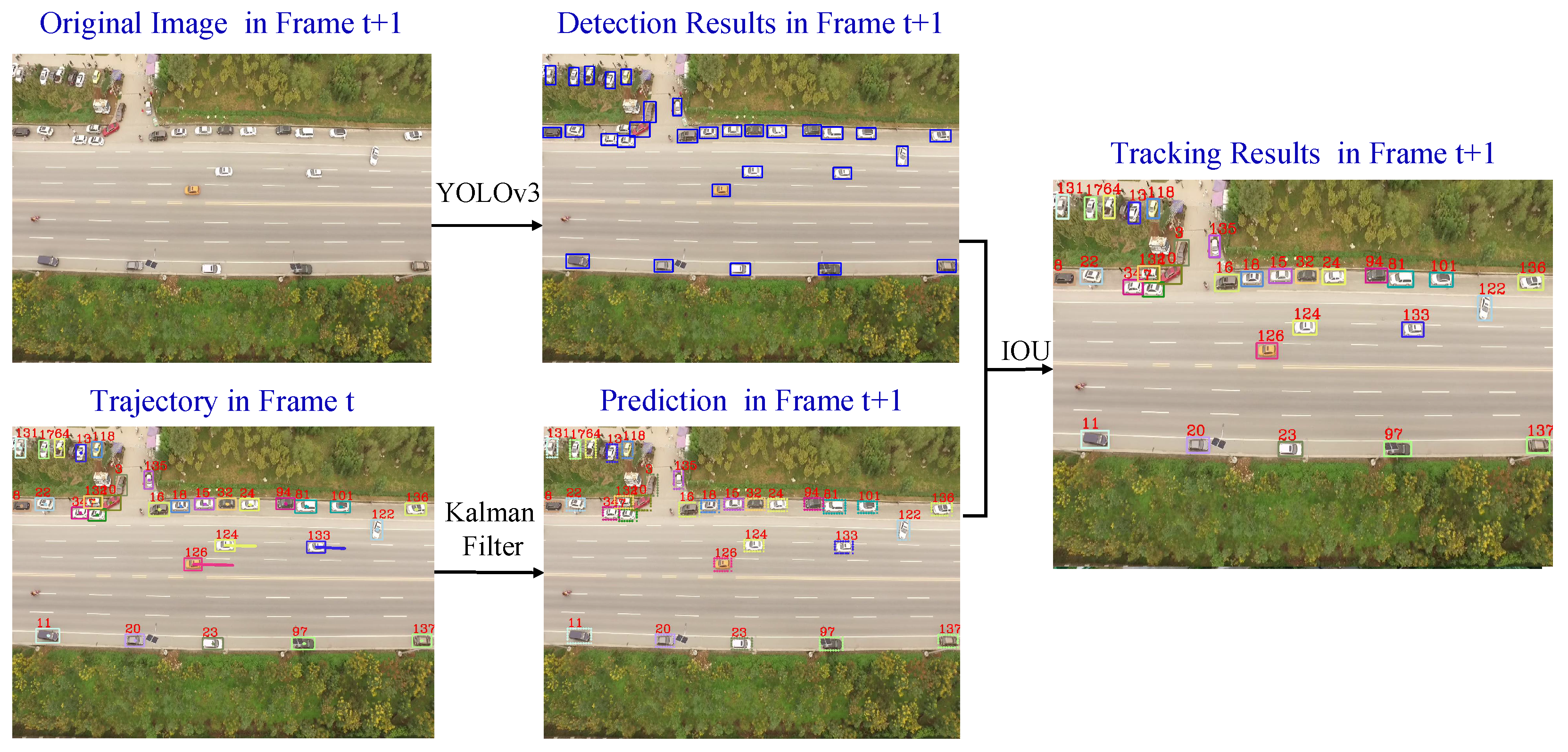
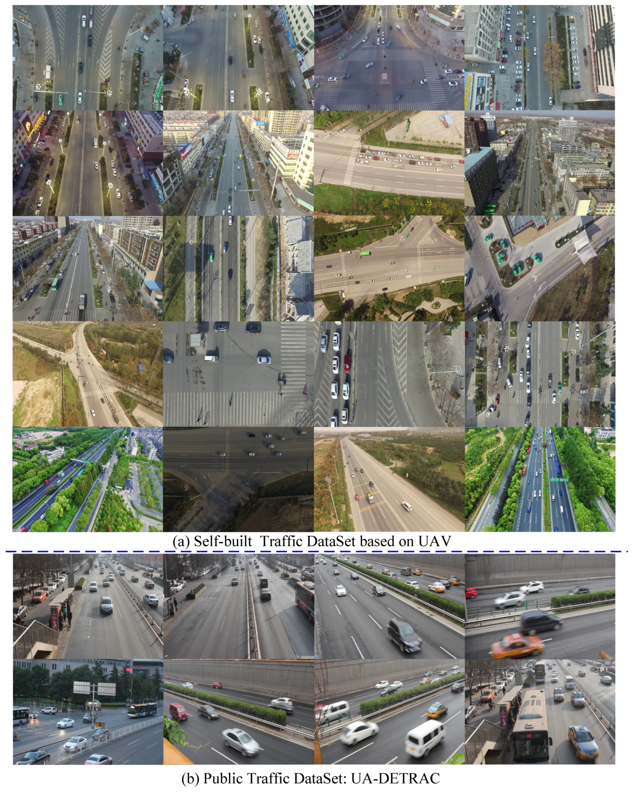
- First, we built a traffic training dataset for vehicle detection in airborne videos, including aerial images which were captured by the UAV, and images of the public traffic dataset (UA-DETRAC). We used this training dataset to generate a neural network model and used the deep learning method to improve the vehicle detection rate in aerial video. Moreover, we established a test dataset for system performance evaluation, which consisted of five aerial scenarios, each with more than 5000 images. Then, we obtained a series of positions for each vehicle in the image through the tracking-by-detection algorithm.
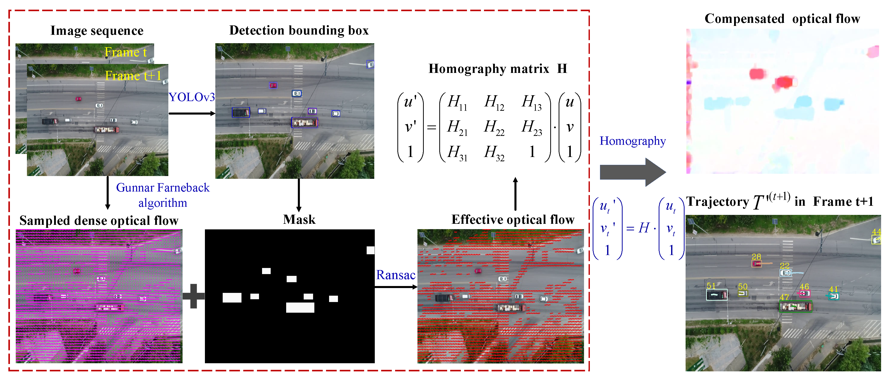
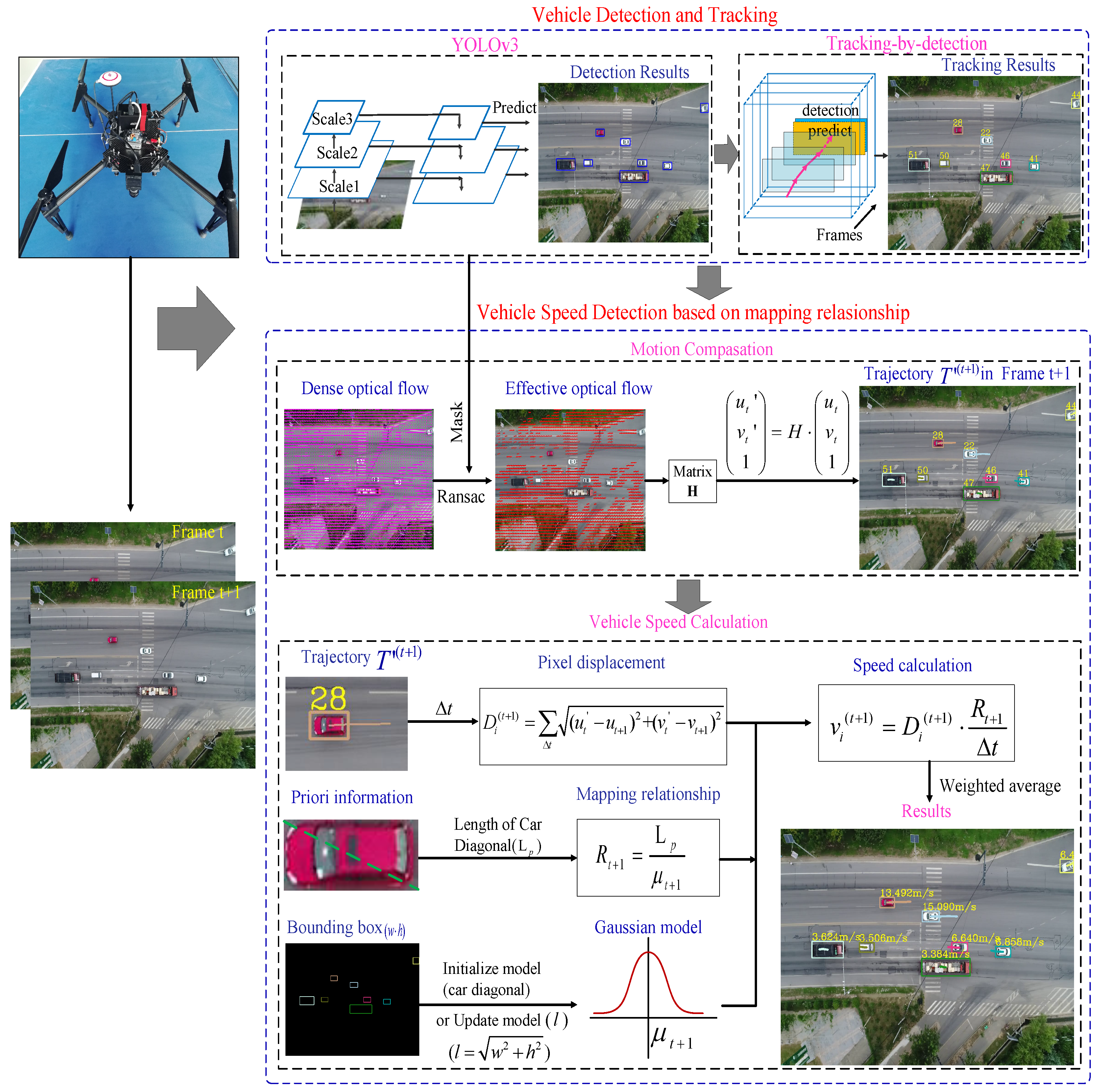
- Second, we formed an adaptive framework for multi-vehicle ground speed estimation in airborne videos. In this framework, based on the detection and tracking results, we first eliminated the influence of the detected target and utilized the motion compensation method based on homography to obtain the vehicle trajectories in the current frame and the real pixel displacements. Then, we designed a mapping relationship between the pixel distance and the actual distance to estimate the real displacements and motion speeds of the vehicles. This used the actual size of the car as the prior information and realized the adaptive recovery of the pixel scale at the current time by estimating the vehicle size in the image.
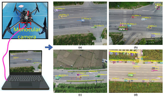
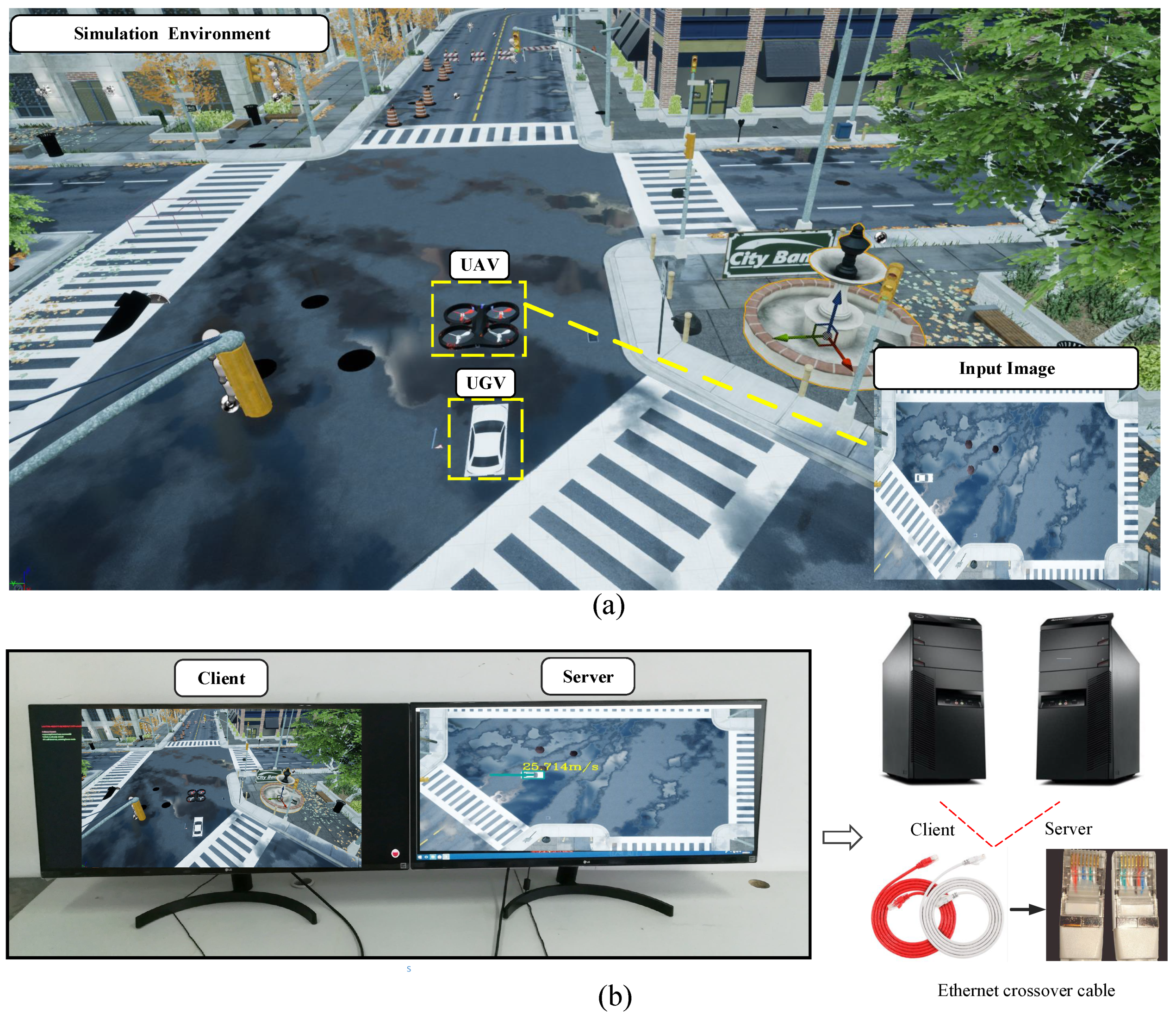
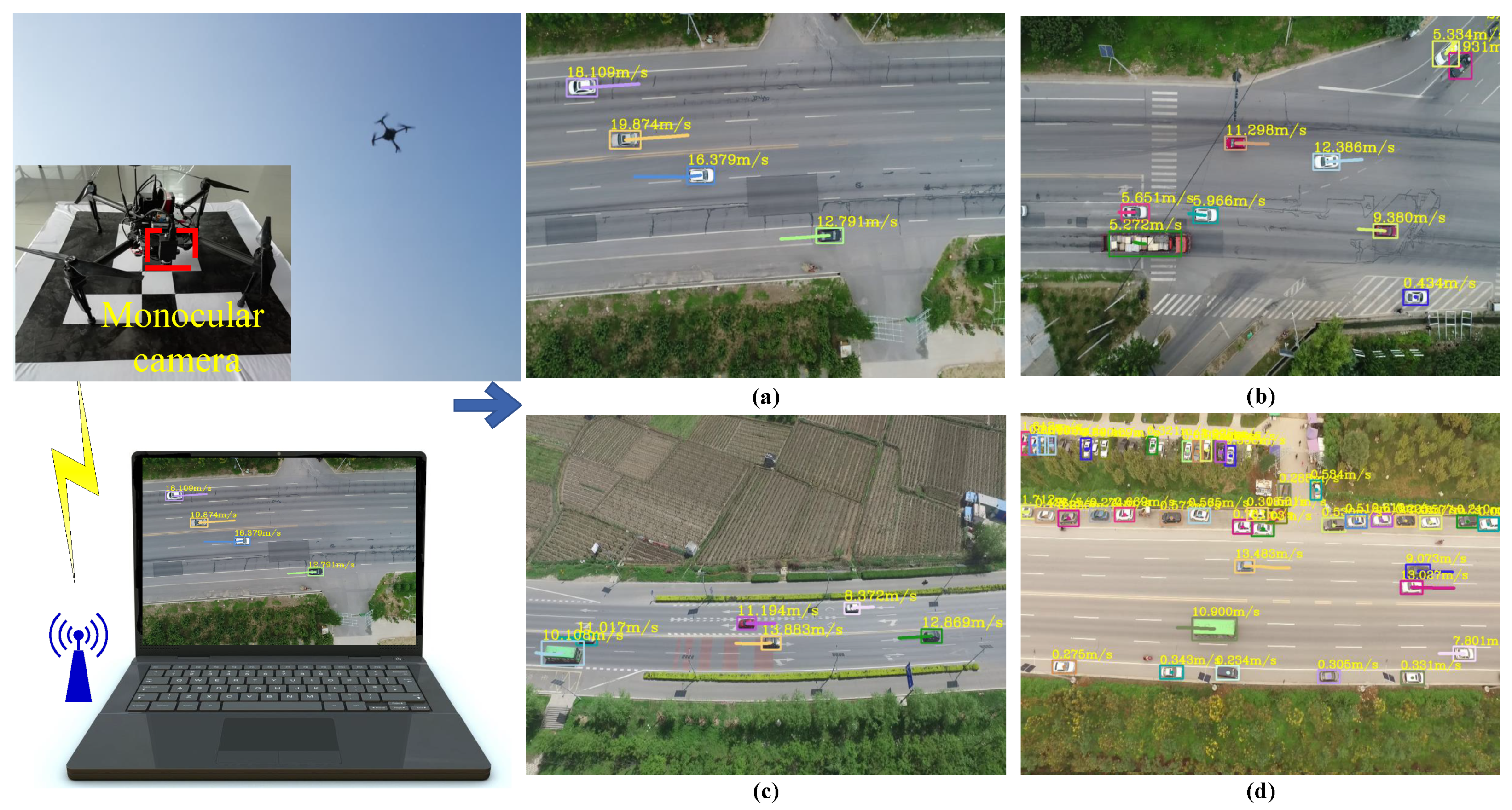
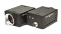
- Finally, we built an adaptive vehicle speed estimation system for airborne video in simulations and in a real environment. The structure of the real system is very simple. It consists of a UAV DJI-MATRICE 100, a Point Grey monocular camera, and a computer. To prove the effectiveness and robustness of the system, we first conducted a large number of simulation experiments on the AirSim platform. The quantitative analysis results were used to verify that the system has a high-speed measurement accuracy. Then, we carried out experiments in real environments, showing that the proposed system has a unique ability to detect, track, and estimate the speed of ground vehicles simultaneously. Moreover, the quantitative experimental results and analysis proved that the system could quickly obtain effective and robust speed estimation results without using auxiliary equipment such as GPS in various complex environments.
2. The Proposed Method
2.1. Vehicle Detection And Tracking
2.2. Motion Compensation of the Vehicle Trajectory
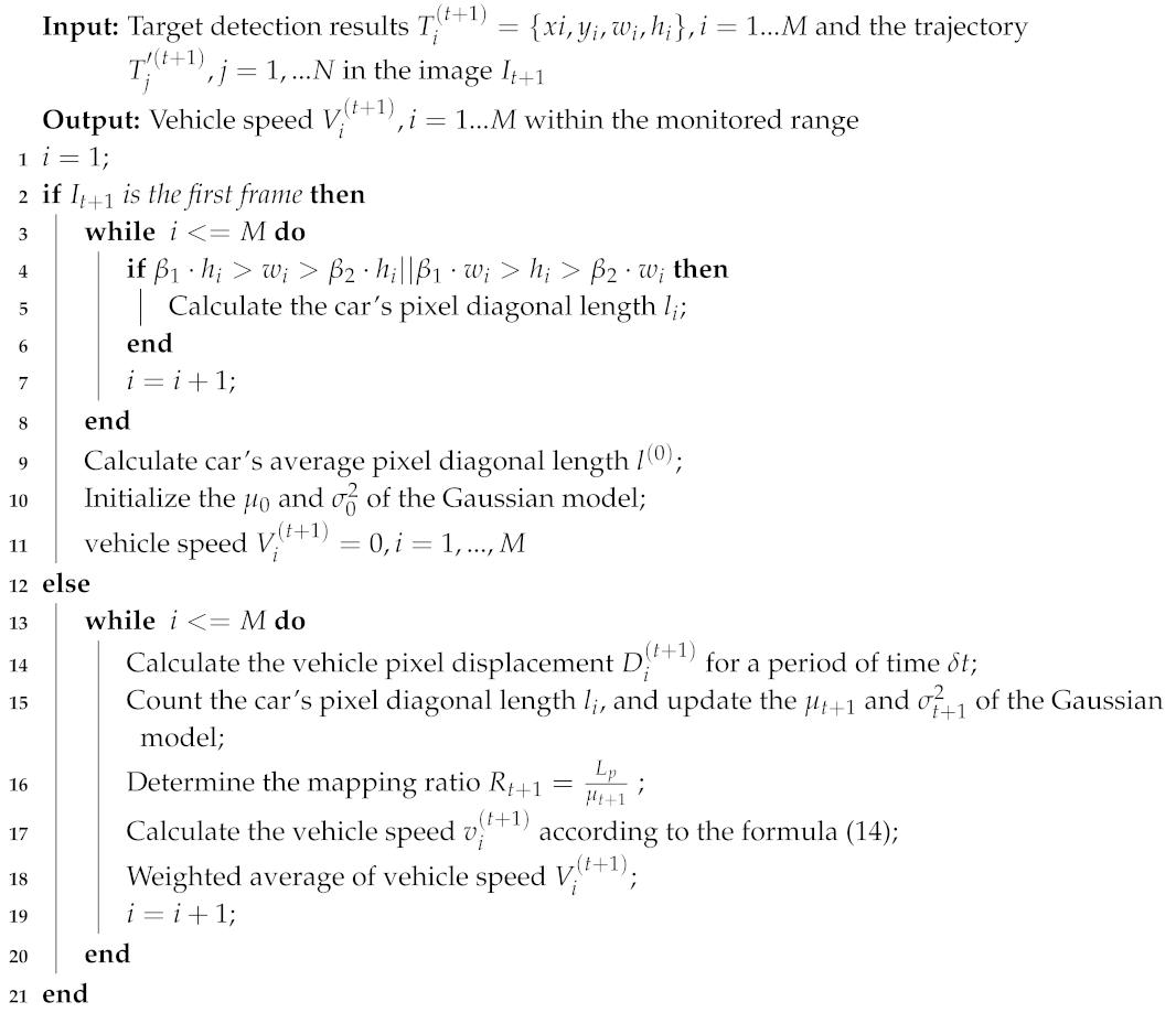
2.3. Adaptive Vehicle Speed Estimation
| Algorithm 1: Vehicle speed calculation method |
 |
3. Experiments
3.1. Traffic Dataset Based On Uav
3.2. Simulation in Airsim
3.2.1. Simulation Platform
3.2.2. Simulation Results
3.3. Real Experiments
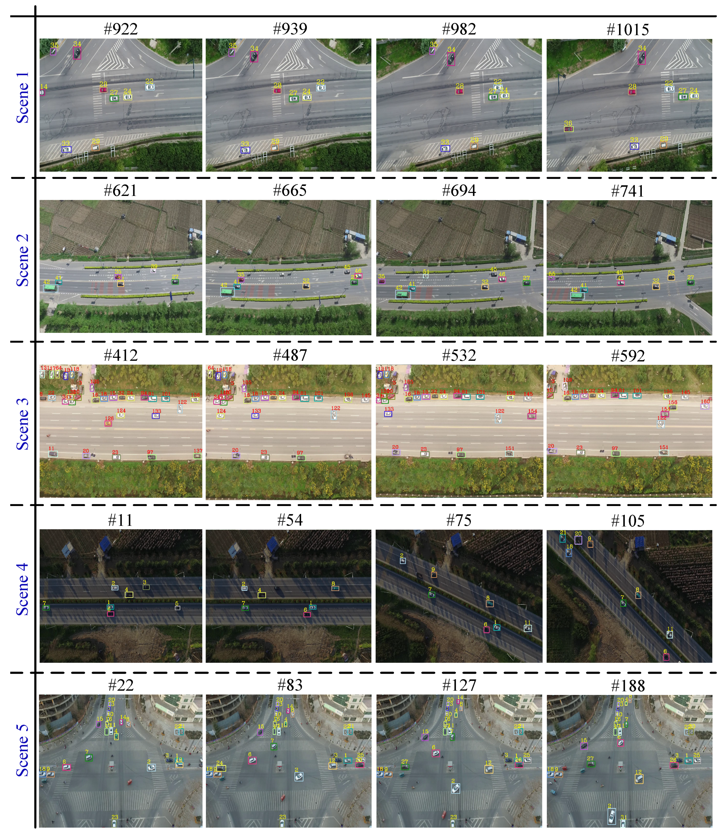
3.3.1. Vehicle Detection and Tracking Experiments
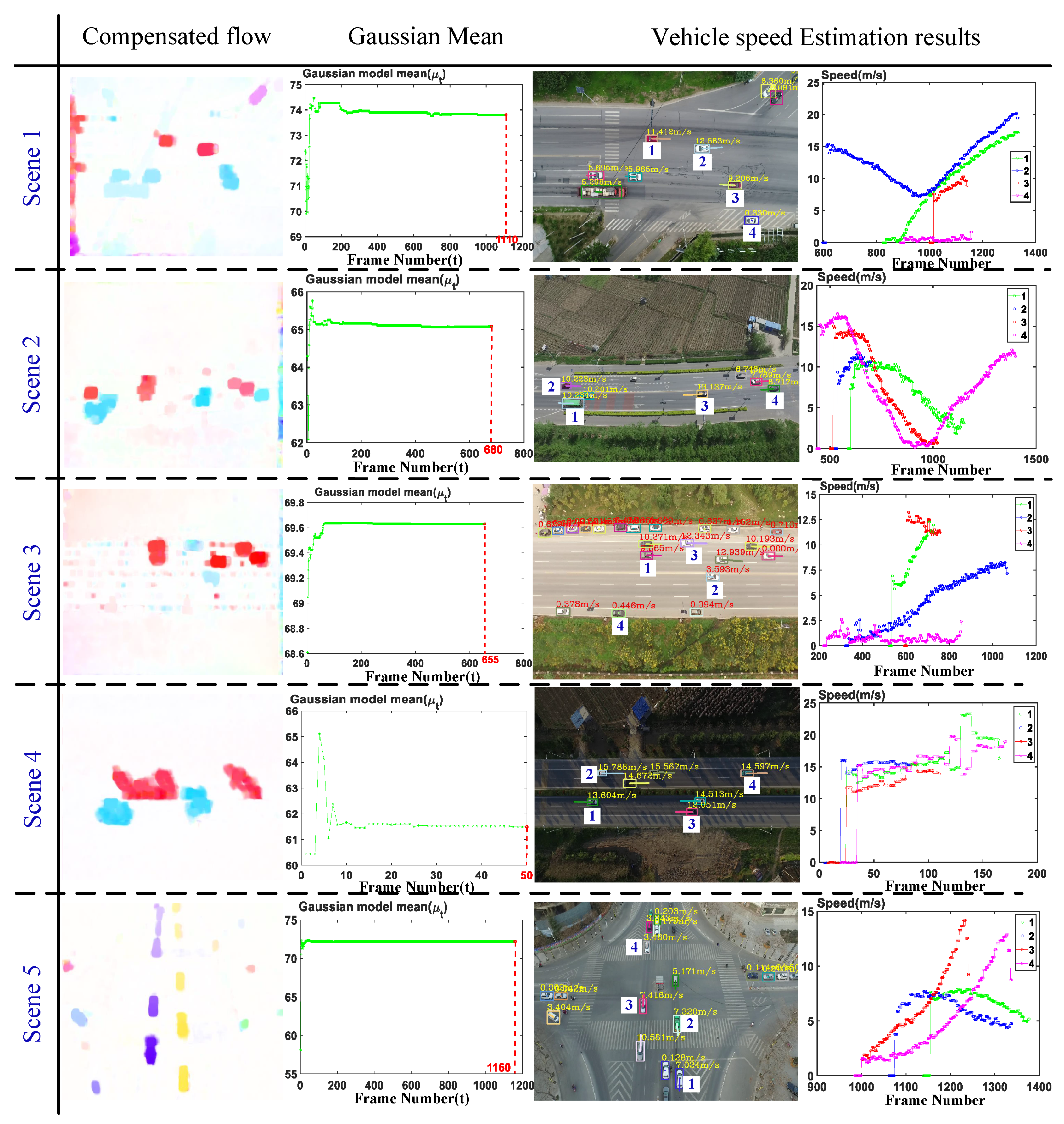
3.3.2. Vehicle Speed Estimation Experiments
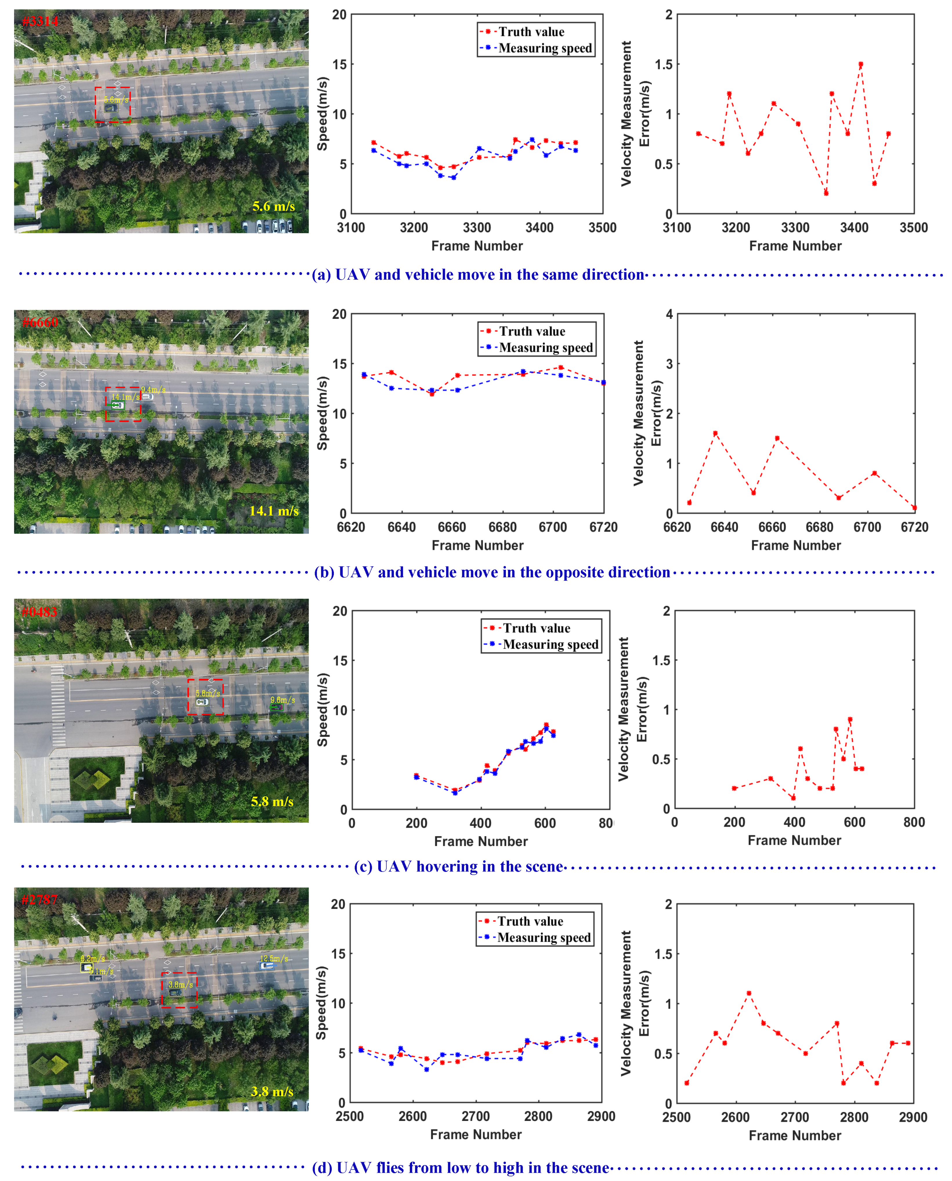
3.3.3. Vehicle Speed Quantitative Experiments
3.3.4. A Priori Information Evaluation Experiments
4. Conclusions
Supplementary Materials
Author Contributions
Funding
Acknowledgments
Conflicts of Interest
References
- Liu, Y. Big data technology and its analysis of application in urban intelligent transportation system. In Proceedings of the International Conference on Intelligent Transportation, Big Data Smart City, Xiamen, China, 25–26 January 2018; pp. 17–19. [Google Scholar]
- Luvizon, D.C.; Nassu, B.T.; Minetto, R. A video-based system for vehicle speed measurement in urban roadways. IEEE Trans. Intell. Transp. Syst. 2017, 18, 1393–1404. [Google Scholar] [CrossRef]
- Yang, T.; Ren, Q.; Zhang, F.; Ren, B.X.H.; Li, J.; Zhang, Y. Hybrid camera array-based uav auto-landing on moving ugv in gps-denied environment. Remote Sens. 2018, 10, 1829. [Google Scholar] [CrossRef]
- El-Geneidy, A.M.; Bertini, R.L. Toward validation of freeway loop detector speed measurements using transit probe data. In Proceedings of the 7th International IEEE Conference on Intelligent Transportation Systems, Washington, WA, USA, 3–6 October 2004; pp. 779–784. [Google Scholar]
- Sato, Y. Radar speed monitoring system. In Proceedings of the Vehicle Navigation and Information Systems Conference, Yokohama, Japan, 31 August–2 September 1994; pp. 89–93. [Google Scholar]
- Lobur, M.; Darnobyt, Y. Car speed measurement based on ultrasonic doppler’s ground speed sensors. In Proceedings of the 2011 11th International Conference The Experience of Designing and Application of CAD Systems in Microelectronics (CADSM), Polyana-Svalyava, Ukraine, 23–25 February 2011; pp. 392–393. [Google Scholar]
- Odat, E.; Shamma, J.S.; Claudel, C. Vehicle classification and speed estimation using combined passive infrared/ultrasonic sensors. IEEE Trans. Intell. Transp. Syst. 2018, 19, 1593–1606. [Google Scholar] [CrossRef]
- Musayev, E. Laser-based large detection area speed measurement methods and systems. Opt. Lasers Eng. 2007, 45, 1049–1054. [Google Scholar] [CrossRef]
- Hussain, T.M.; Baig, A.M.; Saadawi, T.N.; Ahmed, S.A. Infrared pyroelectric sensor for detection of vehicular traffic using digital signal processing techniques. IEEE Trans. Veh. Technol. 1995, 44, 683–689. [Google Scholar] [CrossRef]
- Cevher, V.; Chellappa, R.; Mcclellan, J.H. Vehicle speed estimation using acoustic wave patterns. IEEE Trans. Signal Process. 2009, 57, 30–47. [Google Scholar] [CrossRef]
- Zhang, W.; Tan, G.; Ding, N. Vehicle Speed Estimation Based on Sensor Networks and Signal Correlation Measurement; Springer: Berlin/Heidelberg, Germany, 2014. [Google Scholar]
- Liang, W.; Junfang, S. The speed detection algorithm based on video sequences. In Proceedings of the International Conference on Computer Science Service System, Nanjing, China, 11–13 August 2012; pp. 217–220. [Google Scholar]
- Yung, N.H.C.; Chan, K.C.; Lai, A.H.S. Vehicle-type identification through automated virtual loop assignment and block-based direction-biased motion estimation. IEEE Trans. Intell. Transp. Syst. 1999, 1, 86–97. [Google Scholar]
- Couto, M.S.; Monteiro, J.L.; Santos, J.A. Improving virtual loop sensor accuracy for 2d motion detection. In Proceedings of the 2002 Proceedings of the Bi World Automation Congress, Shanghai, China, 10–14 June 2002; pp. 365–370.
- Alefs, B.; Schreiber, D. Accurate speed measurement from vehicle trajectories using adaboost detection and robust template tracking. In Proceedings of the IEEE Intelligent Transportation Systems Conference, Seattle, WA, USA, 30 September–3 October 2007; pp. 405–412. [Google Scholar]
- Luvizon, D.C.; Nassu, B.T.; Minetto, R. Vehicle speed estimation by license plate detection and tracking. In Proceedings of the 2014 IEEE International Conference on Acoustics, Speech and Signal Processing (ICASSP), Florence, Italy, 4–9 May 2014; pp. 6563–6567. [Google Scholar]
- Wu, J.; Liu, Z.; Li, J.; Gu, C.; Si, M.; Tan, F. An algorithm for automatic vehicle speed detection using video camera. In Proceedings of the International Conference on Computer Science Education, Nanning, China, 25–28 July 2009; pp. 193–196. [Google Scholar]
- Wang, J.X. Research of vehicle speed detection algorithm in video surveillance. In Proceedings of the International Conference on Audio, Language and Image Processing, Shanghai, China, 11–12 July 2016; pp. 349–352. [Google Scholar]
- Llorca, D.F.; Salinas, C.; Jimenez, M.; Parra, I.; Morcillo, A.G.; Izquierdo, R.; Lorenzo, J.; Sotelo, M.A. Two-camera based accurate vehicle speed measurement using average speed at a fixed point. In Proceedings of the IEEE International Conference on Intelligent Transportation Systems, Rio de Janeiro, Brazil, 1–4 November 2016; pp. 2533–2538. [Google Scholar]
- Yang, T.; Li, Z.; Zhang, F.; Xie, B.; Li, J.; Liu, L. Panoramic uav surveillance and recycling system based on structure-free camera array. IEEE Access 2019, 7, 25763–25778. [Google Scholar] [CrossRef]
- Kanistras, K.; Martins, G.; Rutherford, M.J.; Valavanis, K.P. A survey of unmanned aerial vehicles (uavs) for traffic monitoring. In Proceedings of the International Conference on Unmanned Aircraft Systems, Atlanta, GA, USA, 28–31 May 2013; pp. 221–234. [Google Scholar]
- Yamazaki, F.; Liu, W.; Vu, T.T. Vehicle extraction and speed detection from digital aerial images. In Proceedings of the IEEE International Geoscience and Remote Sensing Symposium, IGARSS, Boston, MA, USA, 7–11 July 2008; pp. 1334–1337. [Google Scholar]
- Moranduzzo, T.; Melgani, F. Car speed estimation method for uav images. In Proceedings of the 2014 IEEE Geoscience and Remote Sensing Symposium, Quebec City, QC, Canada, 13–18 July 2014; pp. 4942–4945. [Google Scholar]
- Ke, R.; Li, Z.; Kim, S.; Ash, J.; Cui, Z.; Wang, Y. Real-time bidirectional traffic flow parameter estimation from aerial videos. IEEE Trans. Intell. Transp. Syst. 2017, 18, 890–901. [Google Scholar] [CrossRef]
- Bruin, A.D.; (Thinus) Booysen, M.J. Drone-based traffic flow estimation and tracking using computer vision. In Proceedings of the South African Transport Conference, Pretoria, South Africa, 6–9 July 2015. [Google Scholar]
- Guido, G.; Gallelli, V.; Rogano, D.; Vitale, A. Evaluating the accuracy of vehicle tracking data obtained from unmanned aerial vehicles. Int. J. Transp. Sci. Technol. 2016, 5, 136–151. [Google Scholar] [CrossRef]
- Liu, X.; Yang, T.; Li, J. Real-time ground vehicle detection in aerial infrared imagery based on convolutional neural network. Electronics 2018, 7, 78. [Google Scholar] [CrossRef]
- Xin, Z.; Chang, Y.; Li, L.; Jianing, G. Algorithm of vehicle speed detection in unmanned aerial vehicle videos. In Proceedings of the International Conference on Wireless Communications, NETWORKING and Mobile Computing, Washington DC, USA, 12–16 January 2014; pp. 3375–3378. [Google Scholar]
- Li, J.; Dai, Y.; Li, C.; Shu, J.; Li, D.; Yang, T.; Lu, Z. Visual detail augmented mapping for small aerial target detection. Remote Sens. 2018, 11, 14. [Google Scholar] [CrossRef]
- Shastry, A.C.; Schowengerdt, R.A. Airborne video registration and traffic-flow parameter estimation. IEEE Trans. Intell. Transp. Syst. 2005, 6, 391–405. [Google Scholar] [CrossRef]
- Redmon, J.; Farhadi, A. Yolov3: An incremental improvement. arXiv 2018, arXiv:1804.02767. [Google Scholar]
- Olivier, B.; Marc, V.D. Vibe: A universal background subtraction algorithm for video sequences. IEEE Trans. Image Process. 2011, 20, 1709–1724. [Google Scholar]
- Li, J.; Zhang, F.; Wei, L.; Yang, T.; Lu, Z. Nighttime foreground pedestrian detection based on three-dimensional voxel surface model. Sensors 2017, 17, 2354. [Google Scholar] [CrossRef] [PubMed]
- Tzutalin. Labelimg. Available online: https://github.com/tzutalin/labelImg (accessed on 2 March 2019 ).
- Ren, S.; He, K.; Girshick, R.; Sun, J. Faster r-cnn: Towards real-time object detection with region proposal networks. In Proceedings of the International Conference on Neural Information Processing Systems, Montreal, QC, Canada, 8–13 December 2015; pp. 91–99. [Google Scholar]
- Liu, W.; Anguelov, D.; Erhan, D.; Szegedy, C.; Reed, S.; Fu, C.Y.; Berg, A.C. Ssd: Single shot multibox detector. In Computer Vision—ECCV 2016; Springer: Cham, Switzerland, 2016; pp. 21–37. [Google Scholar]
- Hosang, J.; Benenson, R.; Schiele, B. Learning non-maximum suppression. In Proceedings of the 2017 IEEE Conference on Computer Vision and Pattern Recognition (CVPR), Honolulu, HI, USA, 21–26 July 2017; pp. 6469–6477. [Google Scholar]
- Bewley, A.; Ge, Z.; Ott, L.; Ramos, F.; Upcroft, B. Simple online and realtime tracking. In Proceedings of the 2016 IEEE International Conference on Image Processing (ICIP), Phoenix, AZ, USA, 25–28 September 2016. [Google Scholar]
- Bae, S.H.; Yoon, K.J. Robust online multi-object tracking based on tracklet confidence and online discriminative appearance learning. In Proceedings of the 2014 IEEE Conference on Computer Vision and Pattern Recognition, Columbus, OH, USA, 23–28 June 2014; pp. 1218–1225. [Google Scholar]
- Bochinski, E.; Eiselein, V.; Sikora, T. High-speed tracking-by-detection without using image information. In Proceedings of the IEEE International Conference on Advanced Video and Signal Based Surveillance, Lecce, Italy, 29 August–1 September 2017. [Google Scholar]
- Long, C.; Haizhou, A.; Zijie, Z.; Chong, S. Real-time multiple people tracking with deeply learned candidate selection and person re-identification. In Proceedings of the 2018 IEEE International Conference on Multimedia and Expo (ICME), San Diego, CA, USA, 23–27 July 2018. [Google Scholar]
- Sorenson, H.W. Kalman Filtering: Theory and Application; The Institute of Electrical and Electronics Engineers, Inc.: Piscataway Township, NJ, USA, 1985. [Google Scholar]
- Farneback, G. Two-frame motion estimation based on polynomial expansion. In Proceedings of the Scandinavian Conference on Image Analysis, Halmstad, Sweden, 29 June–2 July 2003; pp. 363–370. [Google Scholar]
- Ua-detrac. Available online: http://detrac-db.rit.albany.edu/ (accessed on 5 February 2019).


| Motion Mode | Average True Speed (m/s) | Average Measured Speed (m/s) | Average Measurement Error (m/s) |
|---|---|---|---|
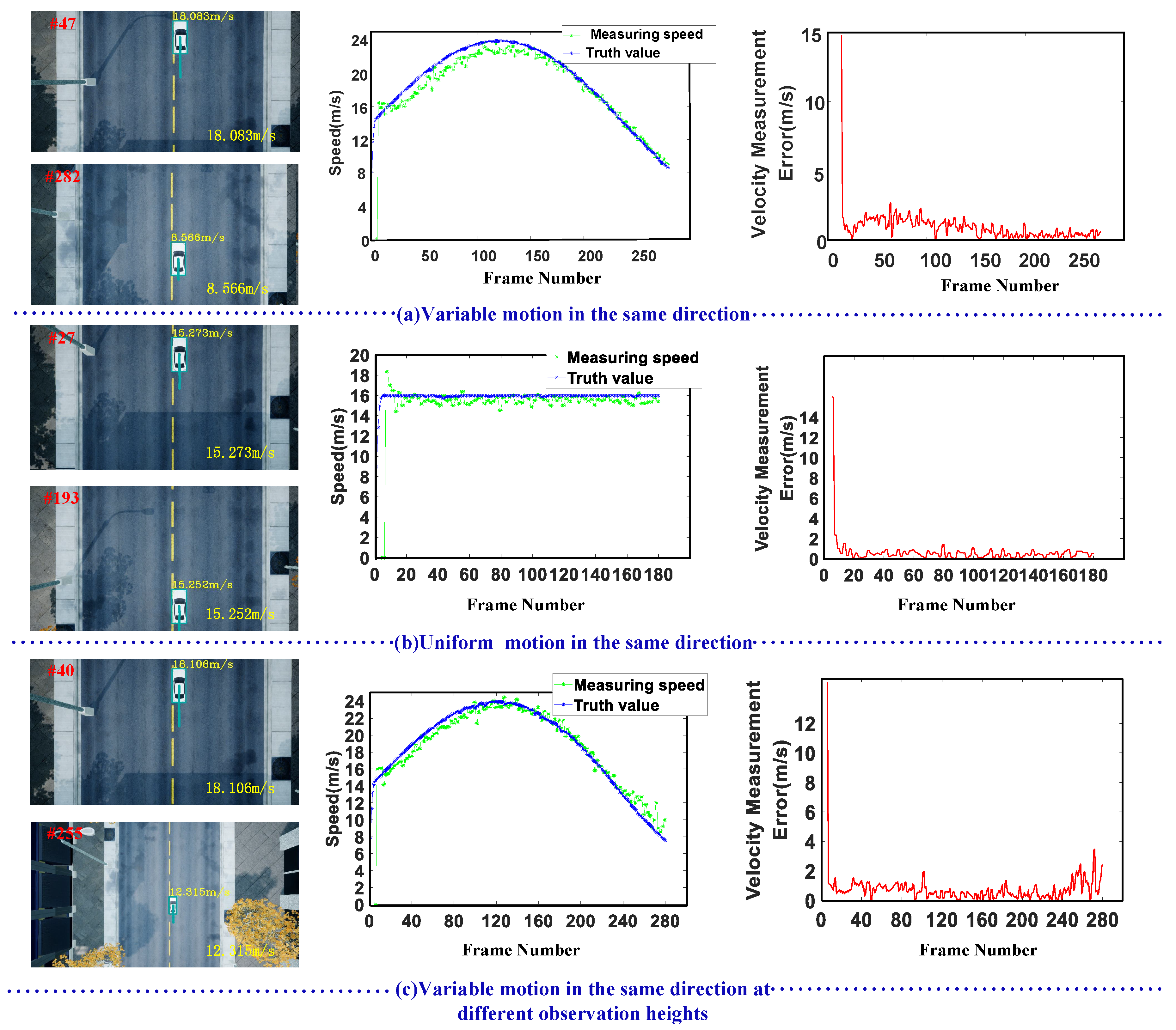
| Variable motion in the same direction | 14.168 | 13.532 | 0.777 |
| Uniform motion in the same direction | 15.952 | 15.081 | 0.924 |
| Variable motion in the same direction and flight altitude is changing. | 18.780 | 18.739 | 0.692 |
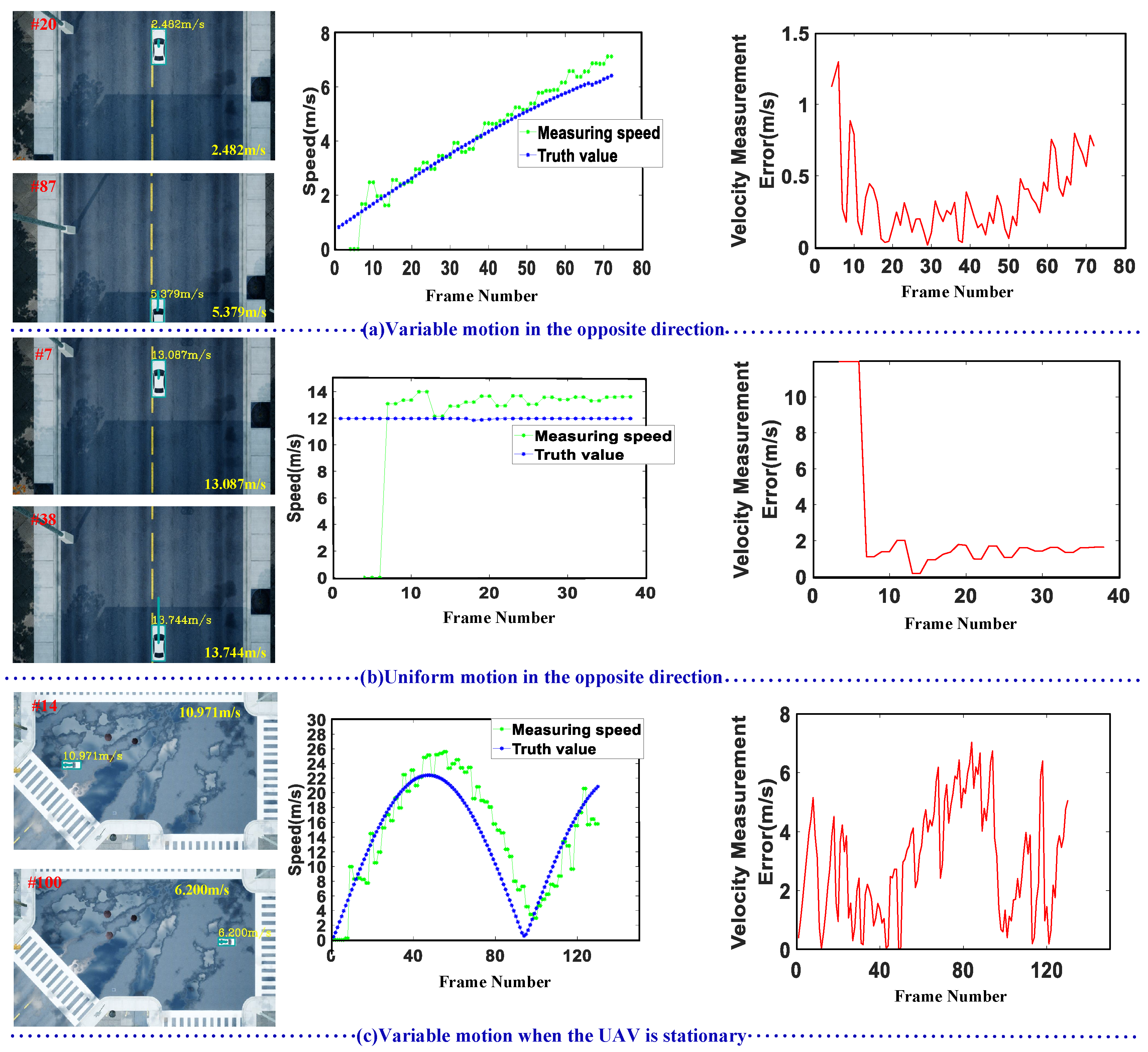
| Variable motion in the opposite direction | 5.557 | 5.876 | 0.419 |
| Uniform motion in the opposite direction | 11.965 | 13.320 | 1.355 |
| Variable motion when the UAV is stationary | 23.197 | 25.196 | 3.481 |
| Point Grey Camera | Specification | Parameter |
|---|---|---|
 | Sensor | CMV4000-3E12 |
| Angle of View | ||
| Resolution | pixels | |
| Frame rate | 60 fps | |
| Power consumption | 4.5 W | |
| Operating temperature | C∼50 C |
| Scene | YOLOv3 [31] | Speed Measurement | System | Fps | ||
|---|---|---|---|---|---|---|
| Tracking | Motion Compensation | Total | ||||
| Scene1 | 45.234 | 0.412 | 42.792 | 23.548 | 57.565 | 17.372 |
| Scene2 | 44.890 | 0.317 | 42.207 | 23.554 | 55.023 | 18.174 |
| Scene3 | 50.674 | 0.700 | 46.565 | 26.712 | 60.369 | 16.565 |
| Scene4 | 46.055 | 0.256 | 43.327 | 23.312 | 59.402 | 16.834 |
| Scene5 | 43.334 | 0.450 | 41.715 | 24.098 | 56.220 | 17.787 |
| Average | 46.037 | 0.427 | 43.321 | 24.245 | 57.716 | 17.346 |
© 2019 by the authors. Licensee MDPI, Basel, Switzerland. This article is an open access article distributed under the terms and conditions of the Creative Commons Attribution (CC BY) license (http://creativecommons.org/licenses/by/4.0/).
Share and Cite
Li, J.; Chen, S.; Zhang, F.; Li, E.; Yang, T.; Lu, Z. An Adaptive Framework for Multi-Vehicle Ground Speed Estimation in Airborne Videos. Remote Sens. 2019, 11, 1241. https://doi.org/10.3390/rs11101241
Li J, Chen S, Zhang F, Li E, Yang T, Lu Z. An Adaptive Framework for Multi-Vehicle Ground Speed Estimation in Airborne Videos. Remote Sensing. 2019; 11(10):1241. https://doi.org/10.3390/rs11101241
Chicago/Turabian StyleLi, Jing, Shuo Chen, Fangbing Zhang, Erkang Li, Tao Yang, and Zhaoyang Lu. 2019. "An Adaptive Framework for Multi-Vehicle Ground Speed Estimation in Airborne Videos" Remote Sensing 11, no. 10: 1241. https://doi.org/10.3390/rs11101241
APA StyleLi, J., Chen, S., Zhang, F., Li, E., Yang, T., & Lu, Z. (2019). An Adaptive Framework for Multi-Vehicle Ground Speed Estimation in Airborne Videos. Remote Sensing, 11(10), 1241. https://doi.org/10.3390/rs11101241