Climate Data Records from Meteosat First Generation Part III: Recalibration and Uncertainty Tracing of the Visible Channel on Meteosat-2–7 Using Reconstructed, Spectrally Changing Response Functions

Abstract

This paper presents a new Fundamental Climate Data Record (FCDR) for the visible (VIS) channel of the Meteosat Visible and Infrared Imager (MVIRI), with pixel-level metrologically traceable uncertainties and error covariance estimates. MVIRI has flown onboard Meteosat First Generation (MFG) satellites between 1982 and 2017. It has served the weather forecasting community with measurements of “visible”, “infra-red” and “water vapour” radiance in near real-time. The precision of the pre-launch sensor spectral response function (SRF) characterisation, particularly of the visible band of this sensor type, improved considerably with time, resulting in higher quality radiances towards the end of the MFG program. Despite these improvements, the correction of the degradation of this sensor has remained a challenging task and previous studies have found the SRF degradation to be faster in the blue than in the near-infrared part of the spectrum. With these limitations, the dataset cannot be immediately applied in climate science. In order to provide a data record that is suited for climate studies, the Horizon 2020 project “FIDelity and Uncertainty in Climate-data records from Earth Observation” (FIDUCEO) conducted (1) a thorough metrological uncertainty analysis for each instrument, and (2) a recalibration using enhanced input data such as reconstructed SRFs. In this paper, we present the metrological analysis, the recalibration results and the resulting consolidated FCDR. In the course of this study we were able to trace-back the remaining uncertainties in the calibrated MVIRI reflectances to underlying effects that have distinct physical root-causes and spatial/temporal correlation patterns. SEVIRI and SCIAMACHY reflectances have been used for a validation of the harmonised dataset. The resulting new FCDR is publicly available for climate studies and for the production of climate data records (CDRs) spanning about 35 years.

1. Introduction

The Meteosat Visible and Infrared Imager (MVIRI) instrument that was operated onboard EUMETSAT’s Meteosat First Generation (MFG) satellites provides an unprecedented opportunity for monitoring climate over a period extending to 35 years. In particular, long-term coverage and frequent temporal sampling in infrared (IR), water-vapour (WV) and visible (VIS) channels at a spatial resolution of 5 km or better, make the implementation of state-of-the-art retrieval algorithms (e.g., [1,2]) for these heritage instruments worthwhile. The MVIRI instrument has been developed to support forecasters at the national weather centres with visually interpretable information about the state of the atmosphere. It acquired one image of the earth disk below the satellite every 30 min with nominal distance between pixel centres of 4.5km at the sub satellite point in the IR/WV bands and 2.25 km in the visible band. While originally being designed in the 1970s, the last of seven MVIRI instruments was launched in 1997. The specifications for the instrument performance as well as the requirements for pre-launch tests have evolved in between the launch dates, hindering the exploitation of 35 years of observations for climate studies up to now.

Among other difficulties, previous studies have particularly pointed out problems with the pre-launch characterisation of the sensor spectral response functions (SRFs) [3,4] as well as the spectral degradation of the MVIRI VIS channel [5,6]. First indications of the pre-launch SRF characterisation problem were reported for the MVIRI VIS channel onboard Meteosat-5 and Meteosat-6 by Y. Govaerts in 1999 [3]. From his paper it became apparent that replacing the SRF of MVIRI on those two satellites by the more precisely measured Meteosat-7 SRF yielded more consistent calibration results. The rationale of this replacement was that the detectors on Meteosat-5-7 were produced in the same batch and that the 4 detectors onboard Meteosat-7 were observed to have very similar characteristics. Despite this improvement, Decoster et al., 2013 [4] found evidence for pre-launch characterisation problems also of the Meteosat-7 instrument by comparing against the HRVIS channel of the Spinning Enhanced Visible and Infrared Imager (SEVIRI) onboard Meteosat Second Generation Satellites. In their paper they show that using the HRVIS SRF (a silicon detector roughly comparable to the MVIRI VIS detectors) for the MVIRI calibration reduces the Root Mean Square (RMS) difference between the two satellites from ~5% to ~3%. The study compared Met-7 to Meteteosat-8 some 5 years after launch of Meteosat-7, where Meteosat-7 had already degraded in the blue considerably [7] and thus in the blue was more similar to the Meteosat-8 than to the Meteosat-7 SRF. In hindsight, this may not be evidence for a prelaunch characterisation problem, but another evidence for spectral degradation. Taking benefit of the long time series of Meteosat-7, Decoster et al., 2013 [4] also discussed spectral degradation of the SRF over time that they observed as a scene-type-dependent instrument degradation. While an overall degradation of the channel responsivity, due to a reduction of the transmissivity of the optical path or a decreasing responsivity of the silicon detectors, had early been observed in the operational calibration facility at EUMETSAT [8], spectral degradation of the SRF was not yet considered. Taking into account the observed spectral degradation through an experimental spectral ageing model [5] further reduced the root mean squared error between the satellites down to ~2%. A later case study about the application of the spectral ageing model at selected target sites on time series of all MFG satellites revealed very good long-term stability metrics [6]. This study, which used a simple linear degradation slope, also pointed out problems with the early Meteosat satellites. However, despite taking into account the effect of spectral degradation through an ageing model, problems with the characterisation of the actual shape of the SRF remained.

While the pre-launch characterisation and calibration of the European Meteosat fleet evolved with time, the international community of satellite operators also developed better means and higher standards for the calibration of instruments on both, polar and geostationary orbiting satellites. The Global Space-based Inter-Calibration System (GSICS), for example, is an international collaborative effort, which aims at ensuring consistent accuracy among space-based observations worldwide for climate monitoring, weather forecasting and environmental applications [9]. Most imagers on past meteorological geostationary satellites were equipped with an onboard calibration blackbody for their infrared channels. In contrast to the infrared channels, these imagers lacked an onboard calibration device for the visible channels.

In the literature different methods are presented for the calibration of visible channel radiances onboard geostationary satellites. Vicarious calibration methods compare observed radiances against modelled radiances over well-known targets, such as stable desert targets [8] or moon targets [10]. A limitation of these methods is that they assume that the surface reflectance functions are well known and invariant in time, which has to be carefully evaluated. Problems arise, for example, due to variations in viewing geometry or changes in atmospheric conditions. Simultaneous Nadir Overpass (SNO) methods compare observed radiances from a monitored instrument against observed radiance from a reference instrument that has superior quality [7,11]. With time the quality of visible channel observations from reference instruments, such as MODerate-resolution Imaging Spectroradiometer (MODIS) [7] or the Visible Infrared Imaging Radiometer Suite (VIIRS) on the NOAA/NASA Suomi NPP (National Polar-orbiting Partnership), improved significantly. In particular the use of onboard solar diffusers helped to meet the calibration accuracy requirement of 2% [12,13], which is much better that the requirements for the visible channels on MVIRI of 10% [14] or Spinning Enhanced Visible and InfraRed Imager (SEVIRI) onboard Meteosat Second Generation (MSG) of 5% [8]. The SNO comparisons against more recent and higher quality imagers like MODIS on Terra and Aqua or VIIRS on Suomi NPP help to improve the accuracy (or decrease the bias) of the calibration from satellites that were not equipped with an onboard solar diffusor [7,15]. However, it needs to be noted that the monitored and the reference instruments often have different SRFs, making inter-comparisons of the radiances a challenging task, particularly in the VIS spectrum. In addition, the reference instruments have their own uncertainties. For example, due to uncertainties of the onboard calibration device (e.g., solar diffusor); uncertainties of the SRFs; or uncertainties in the SNO matches between the monitored and reference instrument. The most preferable method of calibration would be a comparison against SI-traceable instruments that serve as absolute calibration references, such as CLARREO [16] or TRUTHS [9]. These instruments are not yet in orbit though.

With the advent of space-born visible spectrometers, such as the SCanning Imaging Absorption spectroMeter for Atmospheric CartograpHY (SCIAMACHY) on ENVISAT, that was operated from 2002 till 2012, it became possible to evaluate the onboard calibration of other instruments by integrating the hyperspectral SCIAMACHY radiance over the SRF of the monitored instrument. The resulting band-integrated radiance mimics the signal that is expected by the monitored instrument and can be compared to collocated radiances that were actually observed by the monitored instrument itself [17]. For example, Roebeling et al. [18] used SCIAMACHY spectra to quantify the uncertainty of their SNO calibration between AVHRR and SEVIRI. Doelling et al. [17] used SCIAMACHY spectra to develop spectral correction factors for satellite imager solar channels to improve the transfer of calibrations from one imager to another. Their paper shows that SCIAMACHY-based spectral correction helps to improve the transfer of calibrations between different instruments. Moreover, Doelling et al. [19] in another publication have proven that ray-matched collocations with SCIAMACHY can be used to assess and improve the quality of the calibration of geostationary VIS channels. While the numerous studies on this topic have proven the need and demonstrated the feasibility of improved inter-calibration and validation of satellite measurements, their accuracy still depends heavily on the knowledge about the SRF of the monitored instruments.

Today users are increasingly demanding satellite data that are fit for quantitative exploitation with a thorough characterisation of the measurement uncertainty, both in terms of magnitude and correlation in space, time and wavelength. This is addressed in the FIDelity and Uncertainty in Climate data records from Earth Observation (FIDUCEO) project of the EU Framework Program for Research and Innovation. FIDUCEO started in 2015 with the aim to use rigorous metrology techniques (measurement science techniques) to produce key Fundamental Climate Data Records (FCDRs) with traceable and propagated radiance uncertainties, including the MVIRI visible channel FCDR. The general principles of this cross-disciplinary approach were recently published by Mittaz et al. [20]. The MVIRI FCDR covers almost 35 years of geostationary satellite observations (1982–2017) from MFG satellites (Meteosat-2,-3,-4,-5,-6,-7). Within this project Govaerts et al. [21] and Quast et al. [22] developed a sophisticated methodology for in-flight reconstruction of the SRFs of the MVIRI visible channel FCDR, that account for both, the problems with the pre-launch characterisation and the spectral degradation of the detectors. Their papers show that the SRFs of the MVIRI instruments are all subject to spectral degradation. By using information from different types of surface targets (ocean, desert and clouds) degradations of different parts of the spectral response function could be modelled and quantified. The MVIRI visible channel FCDR is provided with these reconstructed SRFs that are used for a consistent recalibration of the MVIRI observations collected by the MFG satellites, and for the computation of the top of atmosphere bidirectional reflectance factors. With the minimised error of the SRF characterisation and the same calibration-methodologies and -references applied to all included sensors, the FCDR can be called “harmonised”. This means that unexpected differences between instruments are largely removed while the characteristics of each individual sensor are maintained such that the recalibrated radiances represent the unique nature of each sensor [23]. Along with the measurements, the FCDR also includes rigorously evaluated information on measurement uncertainties on a pixel basis. These uncertainties are traced back to several effects that have distinct physical root-causes and spatial/temporal correlation patterns. Correlations between effects as well as correlations in time and space are considered and provided along with the FCDR. While the FIDUCEO project has been targeting on the visible band of MVIRI, the FCDR also contains the recalibrated IR and WV bands as obtained from EUMETSATs other activities [24].

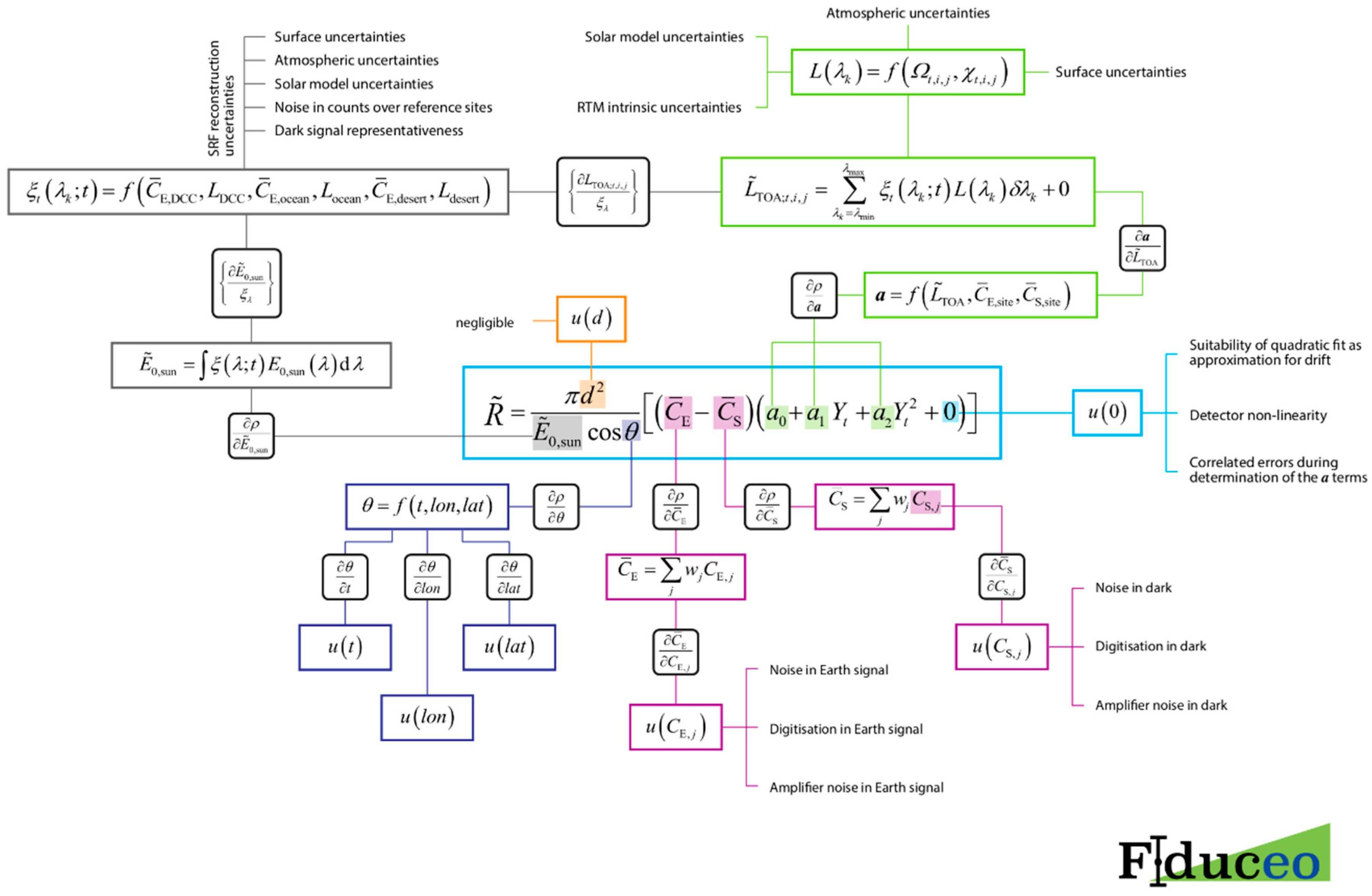
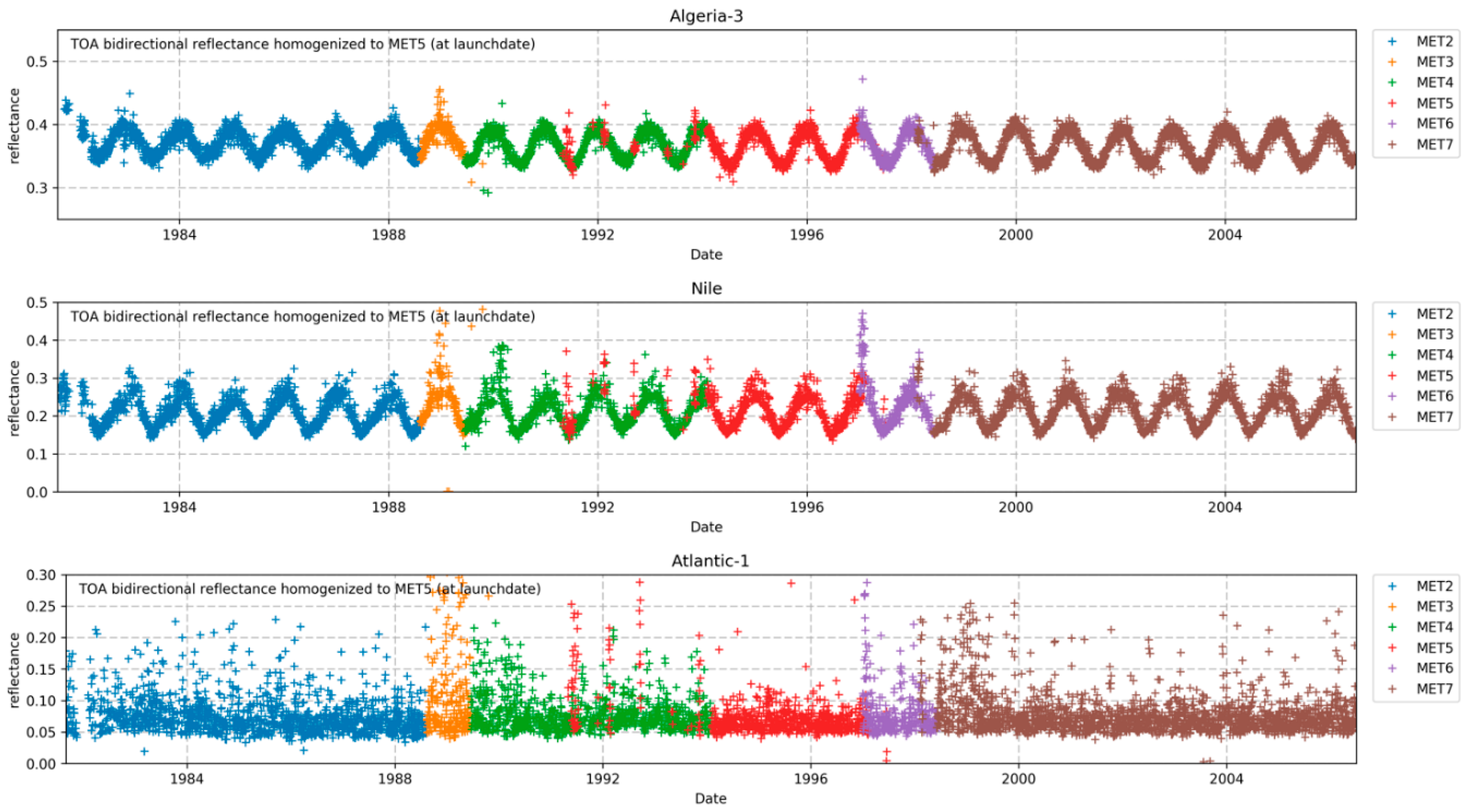
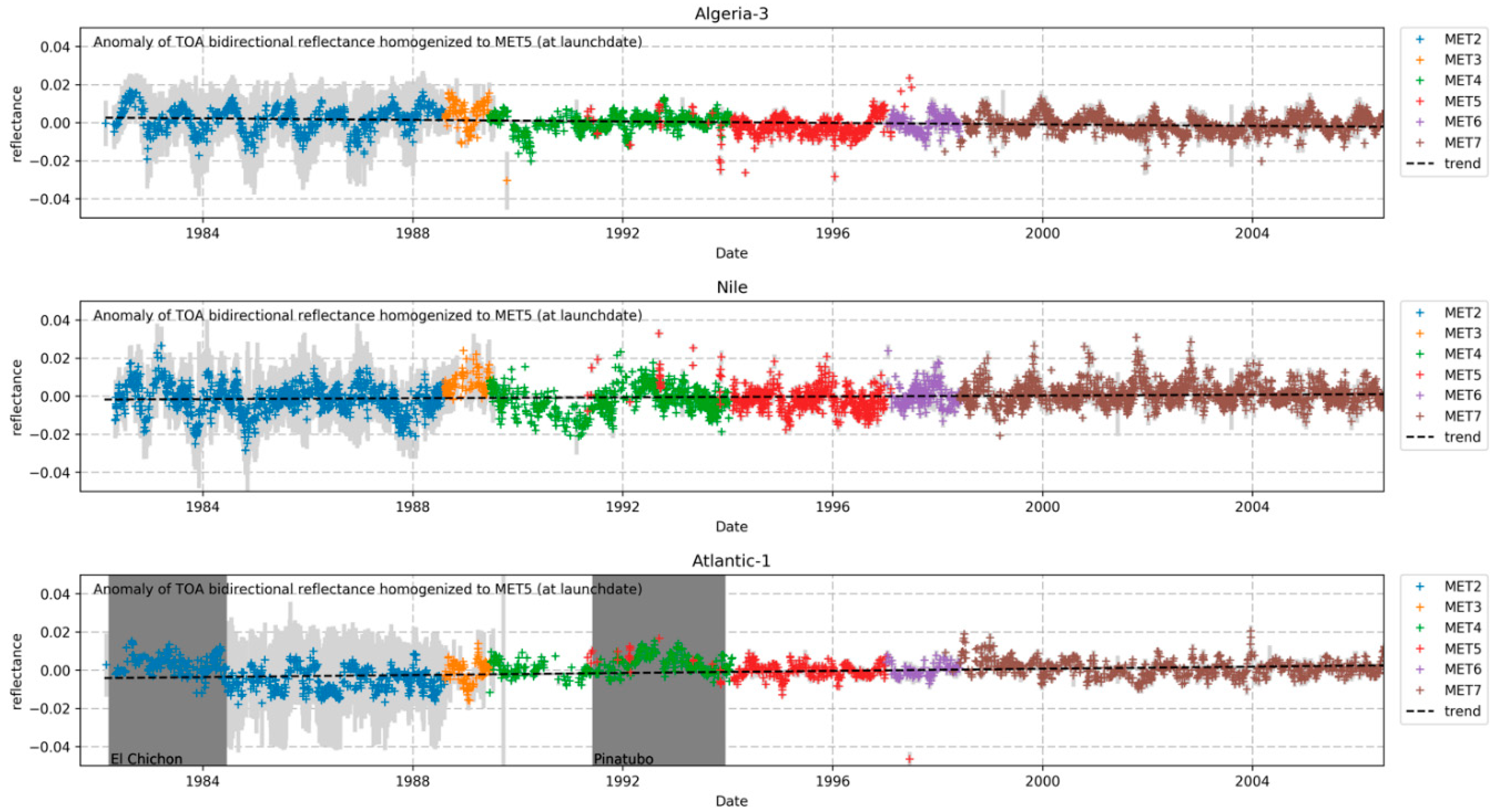
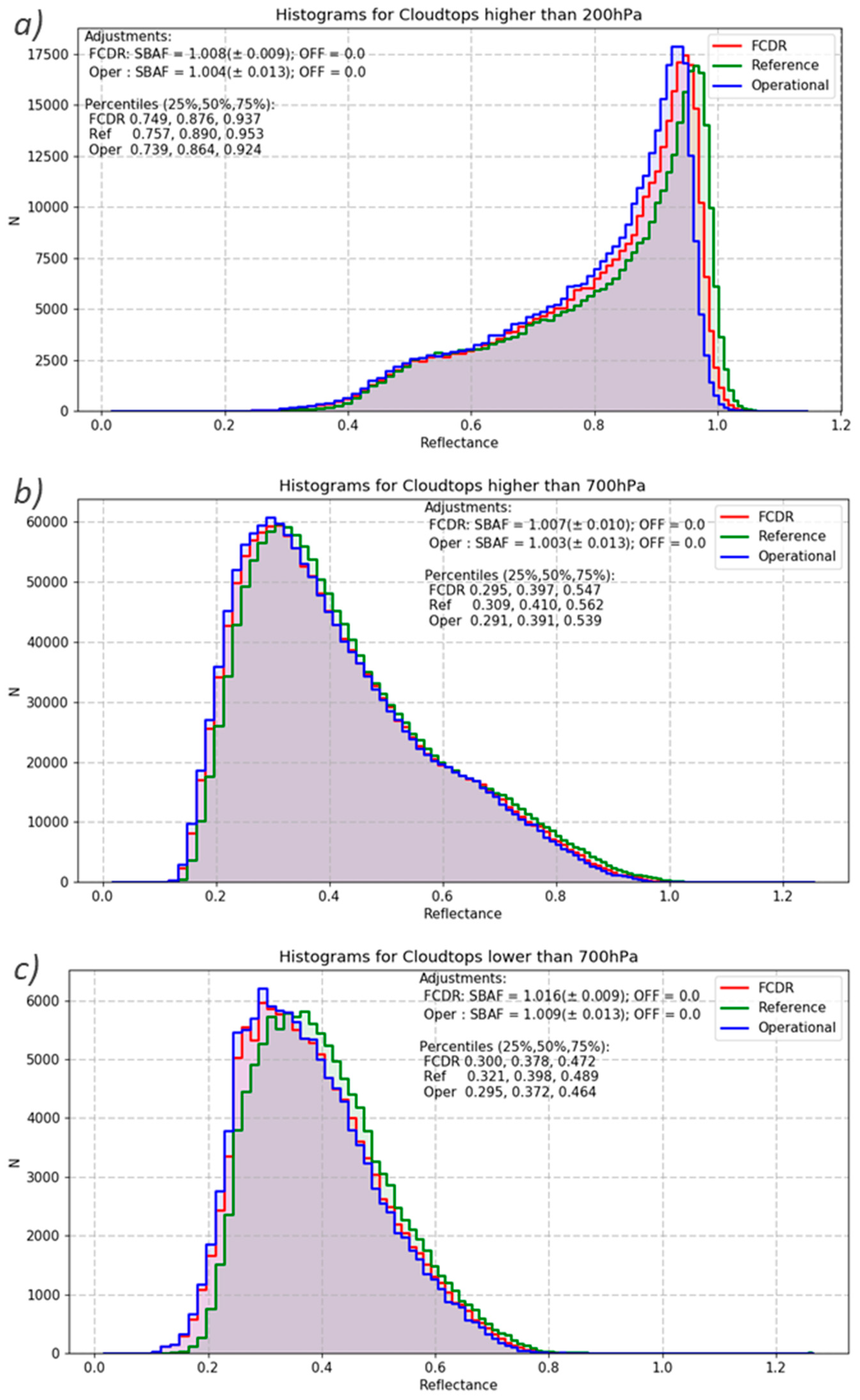
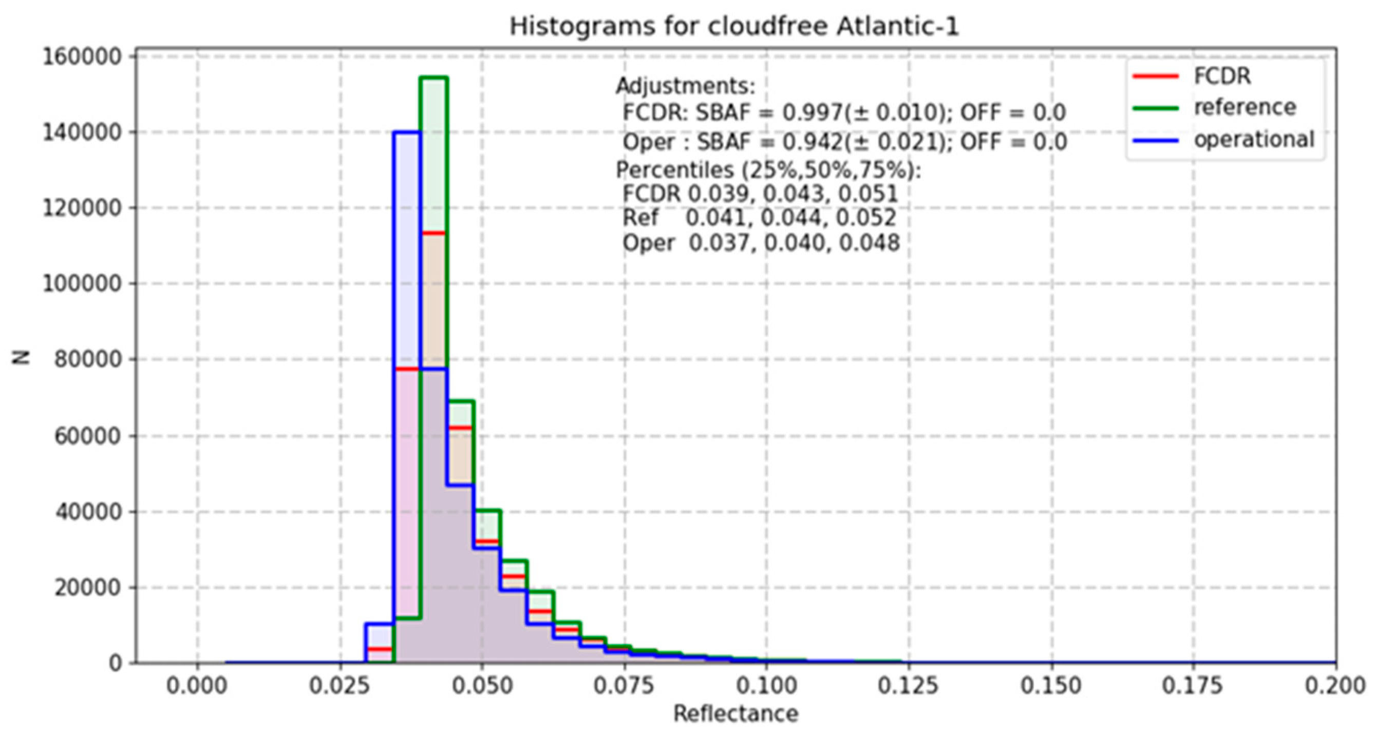
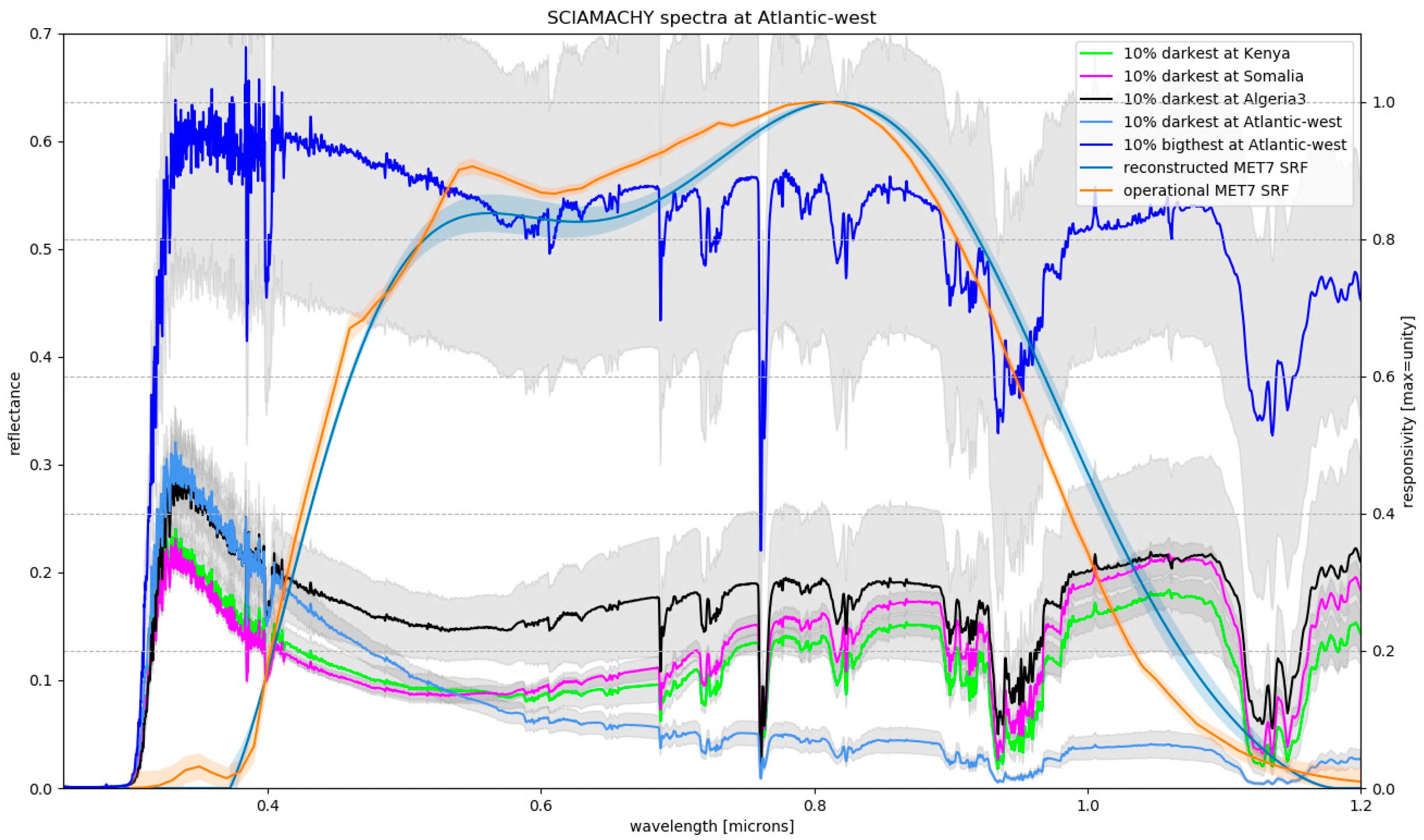
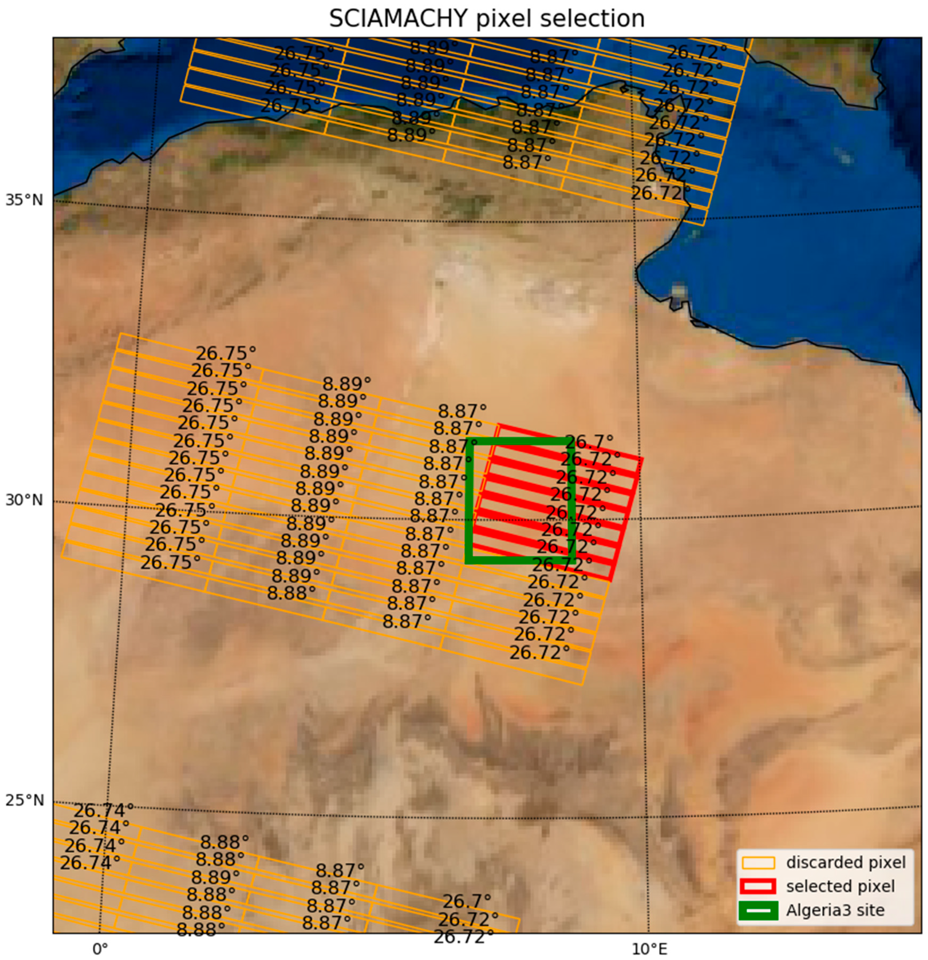
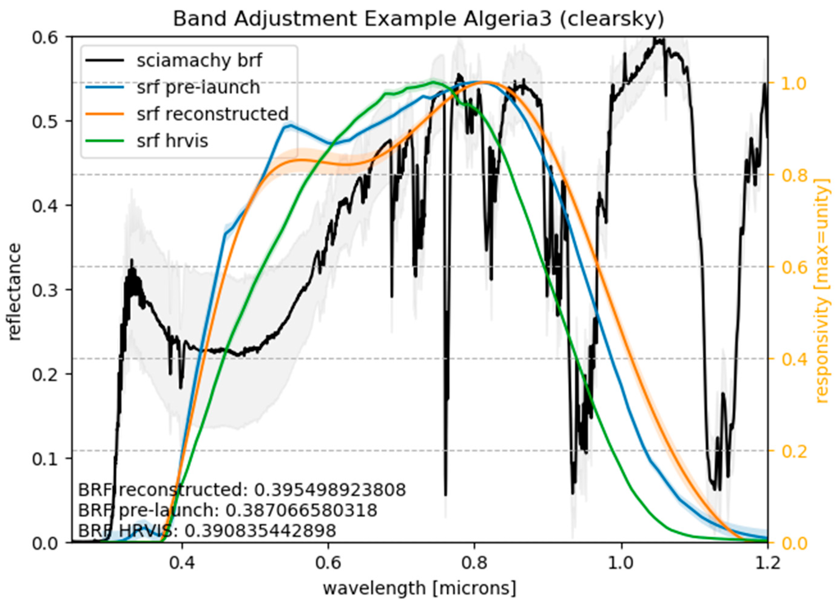
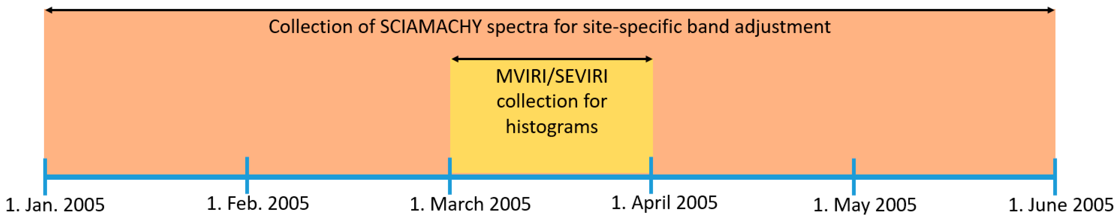
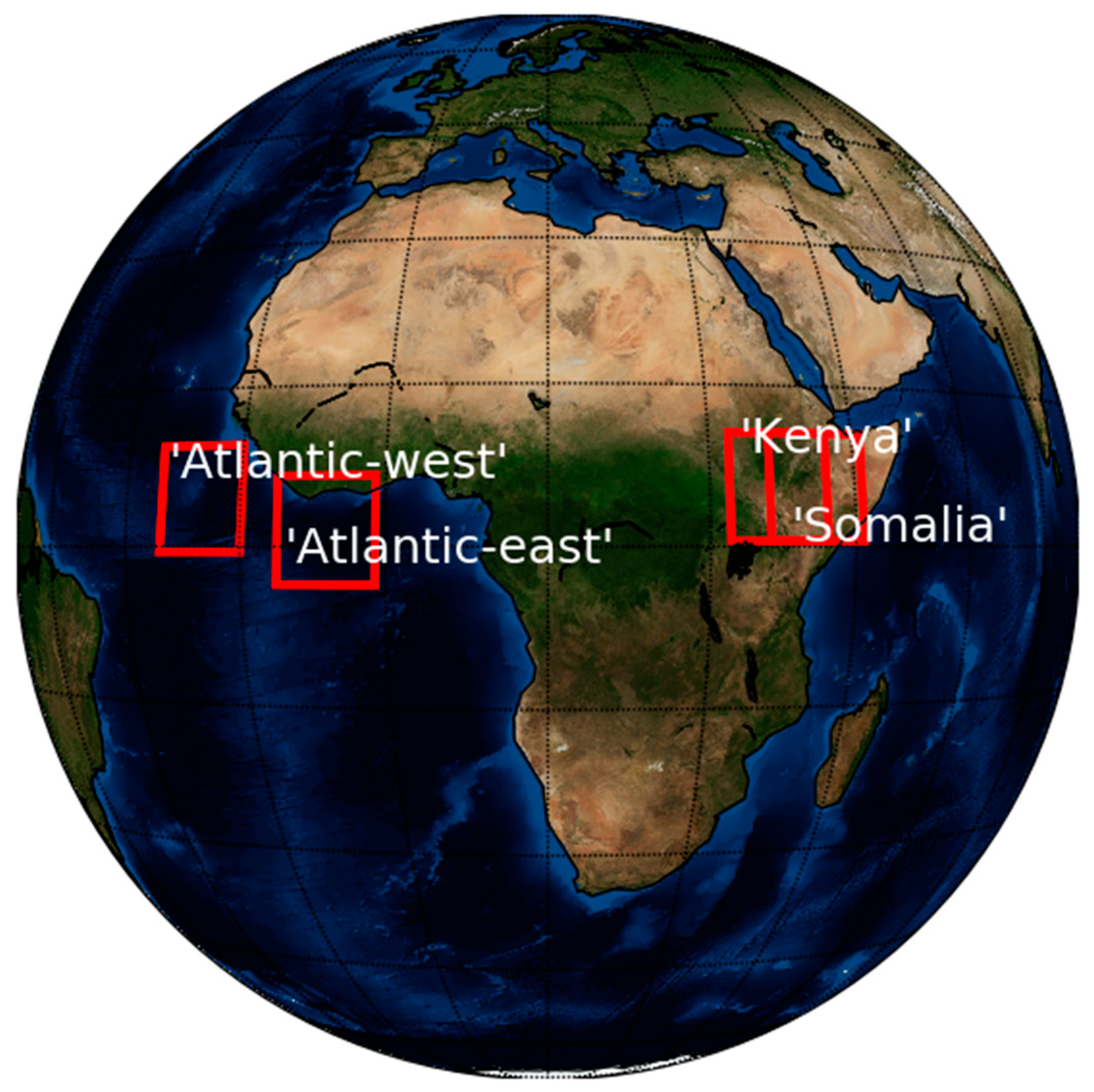
This paper presents the methodology used for the analysis of the measurement uncertainty and for the recalibration/harmonisation of the MVIRI visible channel FCDR from FIDUCEO. The benefit of using the reconstructed SRFs is demonstrated through the use of “homogenised” time series. In contrast to harmonised time series, homogenised time series have the differences between the instruments removed. Homogenisation can only be attempted for time series at sites with known and stable spectral characteristics. The achievements in terms of the calibration accuracy and stability in time and space are validated by exploiting SEVIRI and SCIAMACHY observations over different scene types, such as ocean, agricultural land, desert and deep convective clouds.

The outline of this paper is as follows. Section 2 introduces the monitored satellite datasets and the two reference datasets used in this study. Section 3 describes the methods used within this re-calibration activity. The results are presented and discussed in Section 4. A summary of our study and conclusions are provided in Section 5.

2. Measurements

2.1. MVIRI VIS Observations

MVIRI is a radiometer that was operated on all MFG spacecraft. The first satellite of this kind was launched in 1977, followed by a series of six successors. The constructional design of the spacecraft series and even more of the radiometers changed slightly during the program. The MFG epoch can be divided into three periods:

• The pre-operational period with Meteosat-1 (launch: 23/11/1977), Meteosat-2 (launch: 10/06/1981) and Meteosat-3 (launch: 15/06/1988)
• The slightly improved Meteosat Operational Program (MOP) Meteosat-4 (launch: 19/04/1989), Meteosat-5 (launch: 02/03/1991) and Meteosat-6 (launch: 20/11/1993)
• The Meteosat Transition Program (MTP) with Meteosat-7 (launch: 03/09/1997) which benefitted from an enhanced pre-flight characterisation of the radiometer.

The Meteosat satellites were operated in a geostationary orbit and were designed to provide one image of the earth every 30 min. Continuous data from the sub-satellite position of 0° were collected since Meteosat-2, comprising now more than 24 years of data. In 2006 the 0° service was taken over by Meteosat Second Generation (MSG) satellites. During 1998–2017, Meteosat-5 and 7 were re-located to the east to provide Indian Ocean data coverage (IODC). The visible band of MVIRI essentially consisted of four silicon photodiodes, of which two were active and two were backup. The active silicon detectors responded to the light from the place where the telescope was pointing to. The position of the two active sensors on the radiometer’s focal plane was shifted relative to each other in north-south direction, so that they measured adjacent lines.

The MFG satellites were spin-stabilised satellites and therefore, unlike other three-axis stabilised satellites, they did not need a rotating scan-mirror. The visible images resulted from the interplay of the detectors measuring, the satellite rotating at a defined speed and the telescope tilting to a defined angle. During one revolution of the satellite, each of the two active sensors acquired one scan-line across the earth. The two scan-lines were transmitted to the ground station during that part of the revolution, during which the radiometer was not directed towards the earth. Before transmission the original sensor voltage was truncated into digital count values C. This A/D conversion was done on 8 bits (256 levels) since Meteosat-4. Meteosat-2 and -3 were still encoded to 6-bit values (64 levels). Upon reception in the ground segment, those latter were inflated to the 256-level range of the 8-bit data. For the VIS (IR) detectors each line consisted of 5000 (2500) pixels corresponding to a nadir resolution of 2.25 km (4.5 km) (

Table 1. Spatial and spectral characteristics of Meteosat Visible Infra-Red Imager (MVIRI) visible (VIS), thermal infrared (TIR) and water vapour (WV) channels.

Channel	Sampling Nadir (km)	Nominal Spectral Band (μm)
VIS 0.7	2.25	0.40–1.10
WV 6.4	4.5	5.70–7.10
TIR 11.5	4.5	10.5–12.5

) In the ground segment the raw image lines were combined with metadata into the so-called Level 1.0 format. The processing into the Level 1.5 data format includes the navigation of the images into a georectified grid [25]. For this purpose, information about the orbit attitude and inclination were used to identify the best matching Level 1.0 pixel for each cell in the rectified Level 1.5 grid. The 4 × 4 surrounding Level 1.0 pixels were then averaged using distance-weighted cubic spline interpolation [26]. The accuracy of the georectification was then accessed using a set of Landmarks.

2.2. SEVIRI Measurements

SEVIRI is a radiometer onboard a series of four Meteosat Second Generation (MSG) satellites that are operated by EUMETSAT in a geostationary orbit. In 2002, the first MSG satellite (Meteosat 8) was launched. Similar to the MFG satellites, the MSG satellites are spin stabilised. The SEVIRI instrument operates 12 channels simultaneously. Three of its channels are at visible and near infrared wavelengths between 0.6 and 1.6 μm, eight channels are at infrared wavelengths between 3.8 and 14 μm and one channel is a high-resolution visible (HRVIS) channel. For this study particularly the HRVIS channel is of relevance due to its broad spectral coverage being comparable to the MVIRI VIS channel. As for MVIRI VIS, the detectors employed are silicon photodiodes. In contrast to the latter, however, not only two detectors are operated simultaneously, but an array of 9 detectors. With this setup, the HRVIS channel acquires 9 scanlines during each revolution of the satellite. In this way a fulldisk earth scan can be performed every 15 min, much faster than with MVIRI. During the period 2004–2006, Meteosat-8 was operated at a sub-satellite longitude close to Meteosat-7. This period therefore is predestined for useful comparisons between SEVIRI and MVIRI. The characteristic of four solar channels are summarised in

Table 2. Spatial and spectral characteristics of the four Spinning Enhanced Visible Infra-Red Imager (SEVIRI) visible (VIS) and near infrared (NIR) channels. HRVIS: high-resolution visible.

Channel	Sampling Nadir (km)	Nominal Spectral Band (μm)	Mission Requirement on SNR @1% Albedo
VIS 0.6	3	0.56–0.71	10.1
VIS 0.8	3	0.74–0.88	7.28
NIR1.6	3	1.50–1.78	3.0
HRVIS	1	0.37–1.25	4.3

according to the Meteosat-8 (MSG1) commissioning report [27].

2.3. SCIAMACHY Measurements

SCIAMACHY was a scanning nadir and limb spectrometer covering the ultraviolet (UV) through visible to shortwave infrared (SWIR) spectral range. SCIAMACHY was a joint development of Germany, the Netherlands and Belgium and was launched in February 2002 onboard the ENVISAT platform operated by the European Space Agency (ESA) [28]. About 10 years after launch, on April the 8^th 2012, ESA lost contact with the ENVISAT satellite. ENVISAT was a sun-synchronised polar orbiting satellite with a local equator crossing time of 10:00 AM and an orbital period of about 100 min. SCIAMACHY performed nadir and limb measurements. In limb mode, the instrument observed a certain volume of the atmosphere about 7 min before it was observed in nadir mode. The orbit swath is 960 km wide. The wavelength range covered by SCIAMACHY is 240–2380 nm in eight spectral channels with a spectral resolution between 0.2–1.5 nm. Light that entered the instrument was dispersed using an assembly of prisms and holographic diffraction gratings onto the arrays of 1024 detectors per channel. While reticon photodiodes were used for the five UV-VIS channels, the three SWIR channels were equipped with Indium Gallium Arsenide detectors [29]. The 1024 detectors were sub-divided into clusters that are useful for trace-gas retrieval. As each detector, after the dispersion and bending of the incoming light beam, represented a unique wavelength, the clusters corresponded to wavelength regions. For each of the 56 clusters the integration time could be varied, resulting in various spatial resolutions. This allowed a higher spatial resolution for the most important spectral regions and longer integration times where needed. In order to cover the entire measured spectrum, the measurements of all clusters have to be integrated into the broadest pixel size. Global coverage (in nadir mode) is achieved in six days [30]. Originally designed for studying atmospheric chemistry and aerosols [31], the instrument has proven to be very useful for the cross-calibration, band adjustment and validation of other satellites in numerous studies [17,19,32,33,34]. The Level 1 dataset has undergone several recalibration campaigns. The latest version (V8) of the Level 1b dataset contains all calibration parameters described in [35]. It can be converted into calibrated Level 1c using the CODA software package [36].

3. Methods

3.1. Measurement Equation

As a convenience for the user, the FIDUCEO MVIRI FCDR holds, for each MVIRI Level 1.5 pixel, the recalibrated top of the atmosphere bidirectional reflectance factor as defined in [37]. In the following this term is referred to as reflectance as this is the commonly used term in the remote sensing community. The reflectance is computed using the measurement equation (Equation (1)) with the sun-earth distance d in astronomical units [AU], the band-convoluted solar irradiance ${\tilde{E}}_{0,sun}$ [W m⁻²], the solar zenith angle $\theta$ [rad], the earth count ${\overline{C}}_E$, the mean space count ${\overline{C}}_S$ and the recalibration coefficient $a_{cf}$ [W m⁻² sr⁻¹/C] computed from Equation (10).

$$\tilde{R}=\frac{\pi d^2}{{\tilde{E}}_{0,sun}\cos (\theta )}[({\overline{C}}_E-{\overline{C}}_S)a_{cf}]$$

(1)

The reflectance is provided along with independent and structured uncertainties at pixel level that are rigorously traced from effects of each parameter of the measurement equation (Figure 1). Independent uncertainties are caused by errors that have no spatiotemporal correlation properties. In the MVIRI case this is the noise of the earth counts that is described in Section 3.2. Structured uncertainties come from parameters of the measurement equation that are subject to spatiotemporally correlated errors. The different structured uncertainty effects are described in Section 3.3, Section 3.4, Section 3.5 and Section 3.6. The combination of the effects finally is explained in Section 3.7, Section 3.8 and Section 3.9 describes the methods that were employed for the validation of the new dataset.

3.2. Noise of the Earth Counts

MVIRI VIS earth counts are affected by several sources of noise, mostly the instrument electronics and the coarse digitisation. Other sources of noise, such as photonic noise, were evaluated and considered to be negligible for MVIRI. The electronics noise is assessed in the space corners where all fluctuations of the observations are believed to originate in the instrument. A reason for variations of the electronics noise can be the annual instrument heating cycle due to changes of the solar incidence angle on the satellite [38]. Despite using the space corners for the evaluation of this noise source, it does not represent the uncertainty of the dark signal that is described in Section 3.3. As depicted in Equation (2), the measure in use is the Allan deviation ${\sigma }_{\tau }(C_{Sx})$ [39], computed individually for each of the two detectors and combined with the difference of the mean space count ${\overline{C}}_{Sx}$ of both detectors. The latter accounts for the fact that the earth counts contain the cubic spline interpolated value from a 4 × 4 pixel kernel holding observations of both visible detectors.

$$u({\overline{C}}_{E,e})=\sqrt{\frac{1}{2}({\sigma }_{\tau }{(C_{S1})}^2+{\sigma }_{\tau }{(C_{S2})}^2)+{\left(\frac{{\overline{C}}_{S1}-{\overline{C}}_{S2}}{2}\right)}^2}$$

(2)

The digitisation noise can be assumed to be the standard deviation of a uniform distribution with the width of b digital counts as depicted in Equation (3). For Meteosat-4,-5,-6,-7 b equals 1. Since Meteosat-2 and -3 were encoded only on 6 bits but then inflated to the range of 8 bits, b equals 4 for those satellites.

$$u({\overline{C}}_{E,d})=\frac{b}{2\sqrt{3}}$$

(3)

The uncertainties described in this section are part of the combined independent uncertainty layer provided along with the FCDR (Section 3.7). It can also be accessed by the user as a single-effect uncertainty through an extended version of the FCDR, the so called full-FCDR.

3.3. Uncertainties of the Dark Signal Offset (Space Count)

In the measurement equation, the dark signal ${\overline{C}}_S$ is subtracted from the earth counts in order to remove any variability in the offset of the detector current. The dark signal is estimated by averaging over a large number of space counts in the corners of each image. In contrast to the noise of a single earth count, the uncertainty in the estimation of the dark signal due to noise thus is much smaller than the uncertainty of the earth counts: it averages out and is neglected in the FCDR. However, a substantial contribution to the uncertainty of the dark signal estimation is the fact that the dark signal of two detectors has to be represented by only one value. This could be avoided if the earth counts were not the cubic spline interpolated combinations of both detectors, or if the offset was removed before interpolation. As neither is the case, the uncertainty analysis for the dark signal has to comprise the standard deviation between the means of the two detectors (Equation (4)). Another uncertainty effect is due to the dark signal being determined only once per image while it may vary between the four space corners. The uncertainty analysis thus has to consider the differences between these space corners that are sampled by each of the detectors. Therefore, the standard deviation between the space corner means are considered for both detector 1 (Equation (5)) and detector 2 (Equation (6)). The above described uncertainties can then be combined into a single measure of uncertainty of the dark signal with Equation (7).

$$u({\overline{C}}_{S,d})=\sqrt{\left({({\overline{C}}_{S1}-{\overline{C}}_S)}^2+{({\overline{C}}_{S2}-{\overline{C}}_S)}^2\right)}$$

(4)

$$u({\overline{C}}_{S,s1})=\sqrt{\frac{{\displaystyle \sum _{c=1}^4({\overline{C}}_{S1}(c)}-{\overline{C}}_{S1}{)}^2}{3}}$$

(5)

$$u({\overline{C}}_{S,s2})=\sqrt{\frac{{\displaystyle \sum _{c=1}^4({\overline{C}}_{S2}(c)}-{\overline{C}}_{S2}{)}^2}{3}}$$

(6)

$$u({\overline{C}}_S)=\sqrt{u{({\overline{C}}_{S,d})}^2+u{({\overline{C}}_{S,s1})}^2+u{({\overline{C}}_{S,s2})}^2}$$

(7)

The uncertainty described in this section is part of the combined structured uncertainty layer provided along with the FCDR (Section 3.8). It can also be accessed by the user as a single-effect uncertainty through an extended version of the FCDR, the so called full-FCDR.

3.4. Uncertainties of the Recalibration Parameters

The recalibration of the MVIRI VIS imagery builds upon the operational SEVIRI Solar Channel Calibration System (SSCC) [8]. The SSCC system conducts radiative transfer modelling (RTM) above pseudo invariant calibration sites (desert and sea). The simulated radiances are then related to the corresponding satellite measurements. Outliers, such as observations with cloud- or aerosol-contamination, are rigorously removed [8]. Count-radiance ratios are collected over five-day periods and then combined. Ratios of subsequent 5-day runs are analysed using ODR methods for throughout the lifetime of each satellite to derive the recalibration parameters. Uncertainty propagation through this process is complex and has to consider potential error correlations between the results of the subsequent five-day runs. Therefore, the uncertainty of the five-day count-radiance ratios is separated into four different components: The intrinsic RTM uncertainty, the uncertainties of the surface and atmosphere characterisation, the noise of the satellite counts and the uncertainty of the spectral response function (

Table 3. Uncertainty components of the count-radiance ratios that result from a 5-day calibration run and the correlations between the errors of count-radiance ratios from multiple 5-day calibration runs.

Component	Error Correlation	Justification
Intrinsic RTM uncertainty	Not correlated	Depends on illumination geometry which is different for each 5-day run due to different sets of discarded observations (e.g., due to cloudiness).
Surface characterisation uncertainty	Not correlated	The calibration includes up to 18 desert targets each having its own surface characterisation. The number and weighting the targets varies from 5-day run to 5-day run (e.g., due to cloudiness).
Atmosphere characterisation uncertainty	Not correlated	A systematic bias of the atmosphere parameterisation across the 18 different target sites and multiple days is assumed unlikely.
Spectral Response Function (SRF) uncertainty	Entirely correlated in time and between wavelengths	The SRF characterisation algorithm is performed once per satellite and therefore entirely correlated among all 5-day runs for a satellite.

).

For this study, the SSCC system has been modified to allow for the ingestion of time-variant, reconstructed spectral response functions described in [21,22]. In particular, the propagation of the spectral response function uncertainty has been advanced according to [40] in order to account for the wavelength-dependent error covariance. The error covariance results from the reconstruction methodology [22]. The simulated, band integrated radiance $\tilde{L}$ is computed according to Equation (8) with $L(\lambda )$ denoting the spectral radiance at wavelength $\lambda$, and $\varphi$ denoting the responsivity of the SRF. Correspondingly, the uncertainty component of $\tilde{L}$ that is due to the SRF is computed according to Equation (9) with $S_{\varphi }$ denoting the error covariance matrix of the SRF.

$$\tilde{L}={\displaystyle \underset{\lambda }{\int }L(\lambda )\varphi (\lambda )d\lambda }$$

(8)

$$u_{SRF}(\tilde{L})={\displaystyle \underset{\lambda }{\int }{\displaystyle \underset{{\lambda }^{\prime }}{\int }L(\lambda )S_{\varphi }(\lambda ,{\lambda }^{\prime })L({\lambda }^{\prime })d\lambda d{\lambda }^{\prime }}}$$

(9)

This uncertainty component is then propagated as one component of the uncertainty of each 5-day count-radiance ratio as described in [8].

From the count-radiance ratios of multiple 5-day periods the calibration coefficient at launch ($a_0$) and the grey degradation with time ($a_1$) are retrieved for each satellite. While the degradation was assumed to be well represented by a linear fit in the past, it has become apparent for long-serving satellites, such as Meteosat-2,-5,-7, that the degradation slows down over time. Therefore, a non-linearity term ($a_2$) is added according to Equation (10) where Y denotes the number of years since launch. The three terms $a_0,a_1,a_2$ are valid only in conjunction with the reconstructed, time-variant SRFs and are provided, along with the latter, in the FCDR files. The FIDUCEO +0 term is added to the calibration equation to account for uncertainties of the model that are not represented in the residuals of the fit.

$$a_{cf}=a_0+a_{1}Y+a_2{Y}^2+0$$

(10)

The fitting of the calibration parameters $a_0,a_1,a_2$ is carried out by applying orthogonal distance regression (ODR) on each satellite’s time series of subsequent 5-day calibration results. Weighting is done based on the inverse of the squared combined uncertainty of each run (combined components from Table 3). As common practice, standard uncertainty and covariance of the $a_0,a_1,a_2$ parameters of the ODR fit are computed from the residuals. This is valid for errors that are assumed to be uncorrelated (Table 3: RTM, Surface, Atmosphere), but it does not account for errors that are correlated between calibration runs, such as errors in the characterisation of the SRF. As those errors would not appear in the residuals, they need to be propagated using the +0 term. The +0 term is described in Equation (11). Here, sensitivity matrices C are, as in the ODR model, represented by the inverse of the squared combined uncertainty of each run. The uncertainty matrix U is the correlated uncertainty component, coming from the SRF. The correlation matrix R is assumed to be unity.

$$u(+0)=C\cdot U\cdot R\cdot U^T\cdot C^T$$

(11)

3.5. Uncertainty of the Solar Irradiation

The uncertainty of the band integrated solar irradiation is computed by integrating the solar irradiance spectrum over the SRF. The dominant uncertainty effect on the derived value is the remaining uncertainty from the in-flight SRF reconstruction [22]. As for the simulated radiance above the calibration targets, the uncertainty of the convoluted solar irradiance can be computed by applying the covariance matrix of the reconstructed SRF according to Equation (12). A contribution of the uncertainty of the solar irradiance is not considered in the current release of the FDCR.

$$u_{SRF}( {\tilde{E}}_{0,sun})={\displaystyle \underset{\lambda }{\int }{\displaystyle \underset{{\lambda }^{\prime }}{\int }{E}_{0,sun}(\lambda )S_{\varphi }(\lambda ,{\lambda }^{\prime })E_{0,sun}({\lambda }^{\prime })d\lambda d{\lambda }^{\prime }}}$$

(12)

The uncertainty described in this section is part of the combined structured uncertainty layer provided along with the FCDR (Section 3.8). It can also be accessed by the user as a single-effect uncertainty through an extended version of the FCDR, the so called full-FCDR.

3.6. Uncertainty of the Solar Zenith Angle

The uncertainty of the solar zenith angle is caused by the uncertainties of the geolocation and of the acquisition time. As the accuracy of the acquisition time is better than one second, the impact can be neglected. The geolocation, particularly for poorly navigated images, can have a noticeable impact. The geolocation accuracy is operationally determined in line (l) and element (e) direction using a set of 128 landmarks. The landmarks are located at prominent earth surface features, such as unique coastlines or peninsulas. The geolocation error at each landmark in line- and element-direction is determined based on iterations of shifted correlations with a perfectly located image. The resulting geolocation uncertainty for an entire image is computed as the root mean squared geolocation error of all landmarks. The uncertainty of the solar zenith angle is computed according to Equation (15) with $C_{\theta ,lat}$ and $C_{\theta ,lon}$ being the Monte-Carlo-determined sensitivity coefficients of the solar zenith angle for latitudes and longitudes and $\frac{\partial lat}{u(l)}$ and $\frac{\partial lat}{u(e)}$ denoting the change of latitude that corresponds to the geolocation uncertainty in line and element direction.

$$u_{lat}( \theta )=C_{\theta ,lat}\sqrt{{(\frac{\partial lat}{u(l)})}^2+{(\frac{\partial lat}{u(e)})}^2}$$

(13)

$$u_{lon}( \theta )=C_{\theta ,lon}\sqrt{{(\frac{\partial lon}{u(l)})}^2+{(\frac{\partial lon}{u(e)})}^2}$$

(14)

$$u(\theta )=\sqrt{u_{lat}{( \theta )}^2+u_{lon}{( \theta )}^2}$$

(15)

The uncertainty described in this section is part of the combined structured uncertainty layer provided along with the FCDR (Section 3.8). It can also be accessed by the user as a single-effect uncertainty through an extended version of the FCDR, the so called full-FCDR.

3.7. Combination of Independent Uncertainty Effects

The two significant contributors to the measurement noise, the electronics noise and the digitisation noise, are combined into the independent uncertainty layer as the sum of squares (Equation (16)). The error caused by those effects in a measurement can never be predicted from a previous measurement: Each time it can be considered like an independent draw from the random distribution. The native unit of those two effects are counts. This unit is converted into the unit space of the reflectance by multiplication with the sensitivity coefficient, which is the first derivative of the measurement equation.

$$u_i(\tilde{R})=\sqrt{u{\left({\overline{C}}_{\mathrm{E},\mathrm{e}}\right)}^2+u{\left({\overline{C}}_{\mathrm{E},\mathrm{d}}\right)}^2}\cdot \frac{\partial \tilde{R}}{\partial {\overline{C}}_E}$$

(16)

3.8. Combination of Structured Uncertainty Effects

Structured uncertainty effects are caused by spatially and/or temporally correlated errors. An extreme example of structured uncertainty is the calibration coefficient $a_{cf}$ that is determined only once per satellite. Any error that is made during the calibration process will thus be apparent in every reflectance value of the satellite. A more subtle example is the space count value ${\overline{C}}_S$, which is determined only once per image. The error of this determination is apparent in every reflectance measurement of the same full disk image, but it is independent from the error of the images before and after. Apart from spatial and temporal correlations, the structured uncertainty effects can also be correlated with other effects. For example, both, the uncertainty of the calibration coefficient $a_{cf}$ as well as that of the solar irradiance ${\tilde{E}}_{0,sun}$, are dominated by the uncertainty of the SRF. The correlation of the error between both quantities is therefore high. They were determined by performing Monte Carlo calibration runs with an ensemble of perturbed SRFs. In order to account for the correlations, the structured uncertainties of the reflectance are combined according to Equation (17). In this equation s represents the index of the structured effects $x_s=[a_0,a_1,a_2,+0,{\tilde{E}}_{0,sun},\theta ,{\overline{C}}_S]$, c_s denotes the sensitivity coefficient of the reflectance for each effect, u(x), is the standard uncertainty of an effect and $u(x_s,x_{s^{\prime }})$ is the covariance between two effects. Note that for the representation of the individual error covariances, the recalibration coefficient in this process is represented by the a parameters in Equation (10).

$$u_s(\tilde{R})=\sqrt{{\displaystyle \sum _{s=1}^{n_s}{c}_s^{2}u{(x_s)}^2}+2{\displaystyle \sum _{s=1}^{n_s}{\displaystyle \sum _{s^{\prime }=s+1}^{n_{s-1}}{c}_s{c}_{s^{\prime }}u(x_s,x_{s^{\prime }})}}}$$

(17)

3.9. Validation Methodology

As per definition of a harmonised FCDR [23], the differences in the characteristics of the involved instruments introduce jumps that remain visible even after thorough recalibration. Those jumps are caused by the different shape of the SRF of each MVIRI model. As such, they are not remainders of an incomplete recalibration process, but rather reflect the fact that the measurements are indeed different. Depending on the target in the field of view and its spectral BRDF, the jumps can be larger or smaller, positive or negative. An illustration of the SRFs together with SCIAMACHY spectra from three typical target sites is provided in Figure 2.

Additionally, as a unique feature of the FIDUCEO FCDR, the SRF of the MVIRI visible band is changing with time. This means that after some months in orbit even observations from the same MVIRI instrument have to be considered spectrally different. In the dataset this becomes apparent as long-term trends over certain surfaces. As for the jumps, these trends are not a sign of an invalid recalibration process but rather reflect expected differences of the observations. Any interpretation or validation of the dataset has to consider the different spectral representation of the measurements e.g., by using appropriate spectral band adjustment functions. The spectral band adjustment functions have to be continuously updated to account for the spectral degradation.

The below sections describe the assessments that were made to validate the MVIRI visible channel FCDR from FIDUCEO:

• Evaluation of harmonised and homogenised time-series (Section 3.9.1)
• Comparison against SEVIRI observations (Section 3.9.2)
• Comparison against SCIAMACHY observations (Section 3.9.3)

3.9.1. Evaluation of Harmonised and Homogenised Time Series

The temporal stability of the MVIRI visible channel FCDR is evaluated by analysing time-series of $\tilde{R}$ (reflectance), observed over predefined surface types. In a first step, the harmonised clear-sky time series are compared to expected time series that are exclusively controlled by the shapes of the pre-launch and reconstructed SRFs. For the generation of the expected time series (Figure 8) we use the SCIAMACHY spectra provided in Figure 2. Those spectra are, for each month, convoluted with the applicable SRFs. In a second step, the harmonised clear-sky time series are band-adjusted to the recovered SRF of Meteosat-5 at day-1 as described here below. This process is also referred to as homogenisation [23]. In contrast to harmonisation or recalibration, homogenisation yields time-series where all sensors are forced to (in theory) have the same output, when looking at the same location at the same time. This is achieved by applying corrective terms, so called spectral band adjustment functions, to each recalibrated measurement. It is likely that these corrective terms will not be 100% effective and that the process of homogenisation will add scene-dependent errors to the uncertainty budget that may be difficult to assess. The spectral band adjustment functions for different target-types are obtained from SCIAMACHY spectra collected over these target sites. It should be noted that the need for a-priori knowledge about the spectral characteristics of the observed target renders a global homogenisation in the visible band impossible. Homogenisation of MVIRI VIS observations can only be performed for selected sites where spectral changes (such as unwanted cloud contamination or land cover changes) can be vastly excluded or controlled. The sites considered in this study are listed in

Table 4. Evaluation sites where band-adjusted (homogenised) time series were generated along with spectral characteristics and thresholds for the filtering of SCIAMACHY spectra.

Site	Land Cover Type	Dominant Spectral Contribution	Central Latitude	Central Longitude	Size of Box	thr1	thr2	thr3	thr4
Algeria-3	Desert	Red	30.32	7.66	2° × 2°	0.47	0.38	15	0.5
Nile	Agricultural land	Green	30.5	31.25	0.5° × 0.5°	0.35	0.35	20	0.03
Atlantic-1	Sea	Blue	−22.5	9.5	2° × 2°	0.02	0.053	5	0.02

.

Spectral Band Adjustment (Homogenisation)

An adapted version of the approach described by [17] is used to calculate spectral band adjustment factors that are needed for homogenising the calibration of the MVIRI VIS FCDR over different scene types. The spectral band adjustment factors are determined separately for ocean, desert and agricultural land targets using cloud-free SCIAMACHY spectra that were collected over these targets. Level 1b SCIAMACHY spectra (V8) are provided by the European Space Agency. All calibrations are applied using the SciaL1C Command-line Tool [36]. The SCIAMACHY measurements $P_s(\lambda )$ [photons/(s·cm²·sr·nm)] of the different detectors are averaged to a common integration time and then converted to radiances $L_s(\lambda )$ [W/(m²·sr·nm)] using Equation (18) with h = 6.62607004 × 10⁻³⁴ [Js] and c = 2.998 × 10⁸ [ms⁻¹].

$$L_s(\lambda )=P_s(\lambda )\cdot h\frac{c}{\lambda }$$

(18)

The conversion to reflectance spectra is performed according to Equation (13) using SCIAMACHY measured solar irradiance spectra $I_s(\lambda )$.

$$R_s(\lambda )=\frac{\pi d^2}{I_s(\lambda )\cos (\theta )}{L}_s(\lambda )$$

(19)

An advantage of using reflectance- instead of the radiance-spectra is that systematic errors of the SCIAMACHY measurements cancel out as they are present in the observed radiance spectra $L_s(\lambda )$ and the solar irradiance spectra $I_s(\lambda )$.

SCIAMACHY reflectance spectra that fall with their pixel centre into a predefined lat/lon box around one of the validation sites (Table 4) are considered representative for the target sites (Figure 3). Although spectra were taken from observations collected during the entire lifetime of Envisat (2002–2012), only an arbitrarily thinned dataset was used to reduce CPU demand. The dataset is rigorously cloud filtered using two subsequent tests (

Table 5. Tests for filtering SCIAMACHY spectra. Values for thr1, thr2 and thr3 are given in Table 4.

Test	Condition	Rationale
1	$\frac{{\overline{L}}_s(1120nm:1150nm)}{{\overline{L}}_s(317nm:350nm)}<th{r}_1$	Cloud rejection: Radiance between 1120 nm and 1150 nm is subject of H20 absorption. Clouds reduce the H2O absorption path through the atmosphere and therefore increase this ratio.
2	${\displaystyle \underset{\lambda }{\int }{R}_s(\lambda )\varphi (\lambda )d\lambda }<th{r}_2$	Cloud rejection: The reflectance is convoluted with the spectral response function of the instrument that is the reference for the band-adjustment. Cloud contamination increases the convoluted reflectance in the VIS range.
3	$\left|{\beta }_{scia}-{\beta }_{mviri}\right|<th{r}_3$	Only SCIAMACHY observations with viewing geometries that are comparable to MVIRI geometries are considered. Here β denotes the scattering angles of both SCIAMACHY and MVIRI as computed according to Equation (14).
4	$\sigma (R_M)<th{r}_4$	Only SCHIAMACHY observations with low scene heterogeneity are considered in order to avoid inconsistencies of the band adjustment due to remaining clouds or unwanted surface features.

) that exploit the difference of the penetration depth of the optical path into the atmosphere (Test 1) and the fact that clouds are usually brighter than the earth surface (Test 2). In addition, the scattering angles of MVIRI and SCIAMACHY are compared (Test 3). The scattering angles are calculated from the satellite (θ_v) and solar (θ_sun) zenith angles and satellite (α_v) and solar (α_sun) azimuth angles as (Equation (20)). A final test (Test 4) rejects all SCIAMACHY spectra that are obtained over areas with high scene heterogeneity as e.g., due to remaining cloud contamination or coastlines. To assess scene heterogeneity the standard deviation of all MVIRI pixels $\sigma (R_M)$ that fall within a SCIAMACHY footprint is computed.

$$\beta =\cos ({\theta }_{sun})\cos ({\theta }_v)+\sin ({\theta }_{sun})\sin ({\theta }_v)\cdot \cos (\pi -{\alpha }_v{\alpha }_{sun})$$

(20)

An example of the mean clear-sky spectrum above the Algeria-3 validation site is presented in Figure 4 along with the spectral response functions of the MVIRI VIS and SEVIRI HRVIS bands.

For the computation of the spectral band adjustment factors each individual SCIAMACHY spectrum is convoluted with the SRFs of the reference and the monitored sensors to obtain pseudo reflectances from these two sensors. The spectral band adjustment factors are obtained from the linear regression coefficients of the fit between the pseudo reflectances from the reference and the monitored sensor. Since the SRFs of the monitored sensors used in the MVIRI visible channel FCDR from FIDUCEO vary with time, spectral band adjustment factors needed to be calculated each time the SRF of the monitored instrument changed. An example for the adjustment of Meteosat-2 in 1982 to Meteosat-5 at launch is given in Figure 5. In order to assess the stability of the MVIRI VIS FCDR, the 1982–2006 time-series of the Zero Degree Mission (ZDM) over the validation sites (Table 4) are band adjusted to Meteosat-5 as a reference sensor.

Assessment of Decadal Stability

The assessment of the decadal stability is applied on the homogenised time series above the three validation sites. In a first step an additional cloud filter is applied. The filter uses the distribution statistics from a rolling kernel of 30 days around each reflectance measurement. Measurements that are brighter than the 25% percentile are rejected in order to analyse only measurements that are certainly cloud free. For the Atlantic-1 site also periods with globally elevated aerosol loads due to volcanic eruptions (El Chichon and Pinatubo) are excluded from the stability analysis. Those additional filters are meant to ensure that the computed stability is not corrupted by changes in the performance of the operational cloud mask or by increased Rayleigh-scattering from aerosols. In a second step, the smoothed mean annual cycle is subtracted from the time series in order to get rid of any seasonality. In a third step the measurements are then aggregated to daily means and a generalised linear model (GLM) model is fitted to the deseasonalised time series. The regression slope is evaluated as a measure of the stability in relation to the mean reflectance at each target site. The results of the decadal stability assessment are presented in Section 4.2.

3.9.2. Comparisons with SEVIRI

The SEVIRI sensor onboard the first Meteosat Second Generation (MSG) satellite was operated at a sub-satellite point (SSP) that was only 3° west of Meteosat-7 during the years 2004–2006. For validation purposes particularly the high-resolution visible (HRVIS) band of SEVIRI is useful, due to its similarity with MVIRI VIS. Nevertheless, the true SRFs of MVIRI and SEVIRI are not identical (Figure 4), making a spectral band adjustment (homogenisation) necessary before comparison. As the spectral signatures of different pixels are highly variable in the visible part of the spectrum (Figure 2), the true band adjustment functions are highly variable between pixels. Direct comparisons of a global set of MVIRI pixel measurements with collocated SEVIRI pixel measurements, as presented for the IR bands in [24], are thus not conclusive for the VIS band. Therefore, the comparison approach used in this study relies on measurements over spectrally homogeneous targets (

Table 6. Characterisation of the sites used for the comparison of the SEVIRI HRVIS dataset with the operational MVIRI dataset and the harmonised MVIRI FCDR. The sites and criteria are used for the extraction of suited SCIAMACHY spectra for the homogenisation and for the extraction of SEVIRI/MVIRI observations.

Site	Criterion	Central Latitude	Central Longitude	Size of Box (lat × lon)
Algeria-3	Cloud fraction < 0	30.32	7.66	4° × 4°
High-cloud	Cloud-top-pressure < 200 hPa	0.0	0.0	10° × 10°
Mid-cloud	Cloud-top-pressure 200–700 hPa	0.0	0.0	10° × 10°
Low-cloud	Cloud-top-pressure >700 hPa	0.0	0.0	10° × 10°
Atlantic-1	Cloud fraction < 0	−22.5	9.5	10° × 5°

). For those targets the spectral band adjustment functions can be derived using SCIAMACHY measurements. In order to control the cloudiness of the considered SCIAMACHY spectra, the SEVIRI cloud product is used [2] that also provides an estimate of the cloud-top pressure. To be accepted for the analysis, the footprint of a SCIAMACHY measurement has to be entirely cloud-free (Algeria-3 and Atlantic-1) or homogeneously covered by a cloud with the defined cloud-top-pressure (High-, Mid- and Low-cloud).

The spatiotemporal sampling of MVIRI and SEVIRI is different and close collocations are only available at certain locations of the fulldisk. In order to account for the significant differences of the sampling (~7 min) at the target sites, this study relies on the comparison of histograms that are collected during a longer period. This compensates, for example, for dynamic atmospheric features that are not at exactly the same pixel locations in all datasets. In order to ensure the representativeness of the spectral band adjustment functions for the comparison, the five-month period for the collection of the SCIAMACHY spectra envelopes (Figure 6) the one-month period for the collection of the histograms. Three datasets are compared: (a) the operational Meteosat-7 MVIRI product, (b) the FIDUCEO MVIRI FCDR product and (c) the operational Meteosat-8 SEVIRI HRVIS product. The SEVIRI measurements are considered a superior reference because of the improved pre-launch characterisation as compared to the MVIRI instrument. The MVIRI measurements are band adjusted to the SRF of the HRVIS band using the same methodology as outlined in Section 3.9.1. Histograms from the three datasets are extracted with a maximum time difference of 7 min over four spectrally different targets. The radiometric calibration of the SEVIRI and MVIRI measurements uses the same radiative transfer model and surface and atmosphere parameterisation [8]. Differences between the histograms therefore directly point to problems of the spectral response functions. The improvements of the MVIRI FCDR over the operational MVIRI product are discussed for each region in Section 4.3.

3.9.3. Collocations with SCIAMACHY

The SCIAMACHY spectra can be used to simulate the expected reflectance signal of a monitored broadband visible sensor by convoluting the measured reflectance spectrum from SCIAMACHY with the SRF of the monitored sensor. Collocated pairs of SCIAMACHY simulated reflectances and monitored instrument observed reflectances can only be compared in case they have similar observing times, viewing conditions and illumination geometries (also referred to as ray-matching conditions). As outlined in [29], collocated measurements of SCIAMACHY and a geostationary sensor only occur at certain locations relative to the sub-satellite longitude. This is due to SCIAMACHY’s sun-synchronous orbit and its characteristic pattern of viewing azimuth and viewing zenith angles. The locations with potential for ray-matched collocations between MVIRI and SCIAMACHY are shown in Figure 7 and characterised in

Table 7. Locations of the areas considered for finding potentially ray-matched SCIAMACHY-MVIRI collocations (ZDM and IODC) that are exploited in this study. The viewing zenith angle (VZA) and viewing azimuth angle (VAA) of considered SCIAMACHY observations are indicated.

Location	Central Lat	Central Lon	Surface	Monitored	VZA SCIAM	VAA SCIAM
Atlantic-west	4.5	−20	Sea	MET7 ZDM	~26.7	~102.5
Atlantic-east	1.5	−6	Sea	MET7 ZDM	~8.8	~102.5
Kenya	5.5	37	Semidesert	MET7 IODC	~26.7	~102.5
Somalia	5.5	41	Semidesert	MET5 IODC	~26.7	~102.5

.

The footprint size and acquisition timespan of SCIAMACHY is variable for the different spectral clusters (Section 2.3). The MVIRI SRF spans a very broad domain of the VIS spectrum. In order to be able to convolute the MVIRI SRF with a full SCIAMACHY spectrum, all different spectral clusters of SCIAMACHY need to be integrated to the same footprint size and acquisition timespan. This is done by accumulating the photons at each wavelength over the time interval of the cluster with the longest integration time. As some clusters have very long integration times, only four pixels are available for collocation per scanline. An example of the SCIAMACHY scan pattern over 13 SCIAMACHY scanlines above Algeria-3 is given in Figure 3 along with the viewing zenith angle of each pixel. Representative SCIAMACHY spectra from those sites are provided in Figure 17.

4. Results and Discussion

4.1. Evaluation of Harmonised Time Series

Expected time series, computed by convoluting the pre-launch and reconstructed SRFs with representative mean spectra. They illustrate the expected differences between the reflectance of the different MVIRI sensors and the difference between the FCDR and the operational dataset (Figure 8). The faster degradation of the reconstructed SRFs in the blue part of the spectrum results in increasing (decreasing) reflectance values at the Algeria-3 (Atlantic-1) site over the lifetime of each satellite. An exception is Meteosat 6, where this pattern is inverted. The actually observed time series of clear-sky reflectance extracted from the harmonised MVIRI VIS FCDR match well with those expectations. The most striking features are the jumps between the different sensors. Particularly Meteosat-2 and -3 deviate from the other satellites. At the Algeria-3 target site, with its dominant spectral contribution in the red, the clear-sky reflectance values from Meteosat-2 and -3 are brighter than those of Meteosat-4,-5,-6,-7 (Figure 9). Above the Atlantic-1 target site, with its dominant spectral contribution in the blue, the clear-sky reflectance values from Meteosat-2 and -3 are darker than those from the other satellites (Figure 10). The observed differences can be explained by the differences between the SRFs of Meteosat-2 and -3 and the other satellites (see Figure 2 and Figure 8). From Figure 2 it can be seen that the spectral response of Meteosat-2 and -3 is much weaker between 0.4 and 0.6 μm than the spectral response of Meteosat-4,-5,-6,-7. Therefore, the clear-sky reflectance of Meteosat-2 and -3 measured at Atlantic-1, which reflects most at wavelengths smaller than 0.6 μm, will be lower than from the other satellites. The opposite applies for Algeria-3, which reflects most at wavelengths larger than 0.6 μm. For the green Nile delta (not shown) no noticeable jumps are present. The uncertainties are larger for the older satellites (Meteosat-2 and -3) and reflect the fact that observations from these satellites were encoded on 6 bits only. The seesaw-like pattern of the Meteosat-2 uncertainties may be attributed to the annual cycle of the instrument temperature. This cycle is a result of the satellite being illuminated by the sun from different angles over the year and it is recorded in the instrument telemetry data. Highest instrument temperatures occur during the winter months and highest diurnal amplitudes of the temperatures occur during the eclipse seasons in spring and autumn. Higher instrument temperatures lead to an increase of the noise of the onboard electronics and increase the differences of the sensitivities of the two detectors. In this way the variations in instrument temperatures affect the independent and the structured uncertainty. This influence of instrument temperature variations is smaller for the newer satellites (Meteosat-4,-5,-6,-7) because of enhanced sun protection. The bulging pattern of the independent uncertainty of Meteosat-7 can be attributed to a very different noise level of the two detectors on this satellite. This increases the second term in Equation (2). During June–August the difference in noise level between the two detectors is mitigated by the temperature dependent switches of the Analog-to-Digital converters of the two detection chains [38]. The bulging pattern is only visible at the bright Algeria site, while it is not visible at the dark Atlantic site that is generally very sensitive to instrument noise.

4.2. Evaluation of Homogenised Time Series

The homogenised MVIRI VIS FCDR time series of clear-sky reflectance do not exhibit any prominent jumps between sensors, proving that the FCDR correctly accounts for the real shape of each sensors SRF (Figure 11). Outliers at the Algeria site only occur for the short duration of the Meteosat-3 coverage during winter, pointing to problems of the operational cloud mask. Cloud contamination at the Nile delta is generally higher. Furthermore, impacts of human activities may occur at this site. This leads to a generally higher probability for variability, and that is confirmed by data. The clear-sky reflectance above the Atlantic are, as expected, around 0.05. The high spread of the observed values at this site again points to observations that were not flagged cloudy by the operational cloud mask. In order to exclude the variable performance of the cloud mask from the stability evaluation of the dataset, we implemented a consistent filtering across all satellites as an intermediate step (see Section 3.9.1). After applying this filtering the anomalies of the clear-sky reflectance time series (Figure 12) have been evaluated on their decadal stability. The results reveal very stable behaviour above Algeria-3 and above the Nile delta with trends significantly smaller than 0.7 % decadal change in reflectance (

Table 8. Stability assessment of the harmonised and homogenised FCDR at three reference sites.

Site	Site Mean Reflectance	Stability of Reflectance	Fraction of Site Mean
		[reflectance decade−1]	[%]
Algeria-3	0.36 ± 0.02	−0.0020 ± 0.000	−0.54 ± 0.02
Nile	0.18 ± 0.03	0.0012 ± 0.000	0.66 ± 0.03
Atlantic-1	0.05 ± 0.00	0.0027 ± 0.000	5.26 ± 0.01

). Results for the Atlantic-1 site are slightly worse with around 5% decadal change in reflectance. The main contribution to this change comes from the too dark values of Meteosat-2 (Figure 12). Since the homogenisation should have removed the effects of the different SRFs, this finding indicates a potential overestimation of the Meteosat-2 SRF in the blue region of the spectrum.

4.3. Case-Study Comparison with SEVIRI

The comparisons between the three datasets, i.e., (i) the operational calibrated MVIRI VIS dataset, (ii) the recalibrated MVIRI VIS FCDR, and (iii) the operational SEVIRI HRVIS dataset, show that the trueness of the FCDR has improved above clouds and ocean. Above Algeria-3 the histograms of clear-sky reflectances from both MVIRI datasets do not deviate much from the histogram of the SEVIRI dataset (Figure 13). Only a subtle bright-bias against SEVIRI is observed in both, the operational MVIRI VIS dataset and the MVIRI VIS FCDR. The good fit for this site is attributed to the fact that the three datasets were all calibrated using desert sites with comparable, red spectral characteristics. While this forces all instruments to measure the same over desert-like sites, a bias is introduced as soon as objects in the Field of View (FoV) have a different spectrum, such as clouds and oceans. This is apparent in the cloud histograms shown in Figure 14. This Figure shows the histograms of fully clouded pixels with cloud-tops at three different pressure levels (high clouds (above 200 hPa), middle clouds (between 200 hPa and 700 hPa) and low clouds (below 700 hPa)). From the Figure it can be seen that reflectance values across all cloud levels are lower in the operational MVIRI dataset than in the SEVIRI HRVIS dataset. In the histograms of the recalibrated MVIRI FCDR this dark bias is slightly reduced for low and middle clouds and fundamentally reduced for high clouds. For high clouds, the observed shift towards brighter cloud reflectance values would affect the top of the atmosphere outgoing shortwave radiation by roughly 8 W/m². Similar behaviour is observed over the Atlantic-1 target. Here the histogram from the operational dataset is also darker than that from the SEVIRI dataset (Figure 15) and the histogram from the recalibrated MVIRI VIS FCDR matches much better with the histogram of the SEVIRI dataset. The better match between the FCDR and the SEVIRI dataset is encouraging and confirms that the clear-sky and cloudy reflectances of target sites with different spectral characteristics are better (assuming SEVIRI is the better characterised instrument) represented when using reconstructed SRFs than when using original (operational) SRFs.

4.4. Collocations with SCIAMACHY

The results from the collocations with SCIAMACHY support the findings from the case-study comparison with SEVIRI. For the semi-arid to arid surfaces of the Kenya and Somalia areas the recalibrated FCDR and the operational MVIRI dataset have comparable performance (Figure 16, bottom-panels). To understand this, it is necessary to consider the shapes of the spectra at those locations (Figure 17). The spectral shapes of the Kenya and Somalia areas are relatively close to the desert sites that are used for the calibration of both MVIRI datasets (e.g., Algeria-3). Over these two areas the differences between the spectral signatures mainly occur in parts of the spectrum where the original SRF does not deviate much from the reconstructed SRF.

This is different for the Atlantic areas where the MVIRI FCDR performs significantly better than the operational MVIRI dataset, with regression slopes improving from about 0.97 for the operational dataset to 0.99 for the MVIRI FCDR. For these areas the signal of the large SCIAMACHY footprint includes both, blue clear-sky sea spectra and white cloud spectra. An illustration of the spectra is provided in Figure 17 where the 10% darkest Atlantic spectra represent largely cloud-free observations while the 10% brightest Atlantic spectra represent mainly cloudy observations. The combination of dark ocean surfaces with bright clouds explains the large range of the values at the Atlantic areas. The spectral shape of those observations differs strongly from the calibration sites and thus the results are more sensitive to errors of the SRF. It can be concluded that the use of reconstructed SRFs in the MVIRI FCDR leads to a significant reduction of the dark bias that is observed in the operational MVIRI dataset (Figure 16, top-panels).

5. Summary and Conclusions

This paper addresses four aspects for the realisation of a long-term, stable and ready-to-use MVIRI visible channel FCDR: (i) the improvement of the instrument characterisation though the use of reconstructed SRFs, (ii) the application of a consistent recalibration methodology, (iii) the quantification of traceable uncertainties using metrological techniques, and (iv) the validation of the performance of the FCDR using reference datasets.

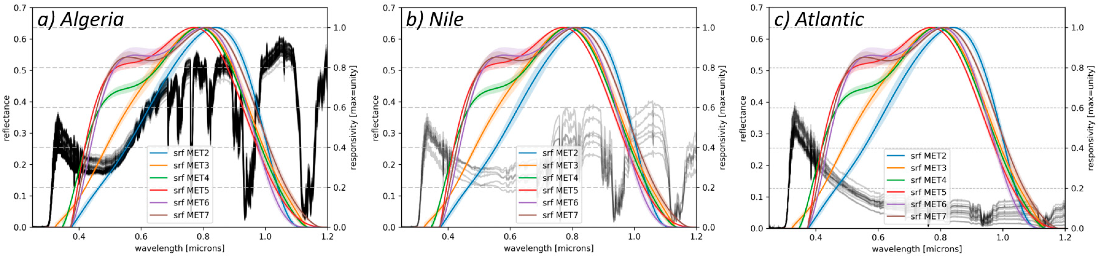
The improvement of the characterisation of the SRF was achieved using the methods described in two companion papers [21,22]. The paper at hand now shows that the reconstructed SRFs can properly account for the differences between the different MVIRI instruments, as well as the spectral degradation of individual instruments with time. For Meteosat-2, it is found that the reconstructed SRF may still slightly overestimate the responsivity of the instrument in the blue part of the spectrum.

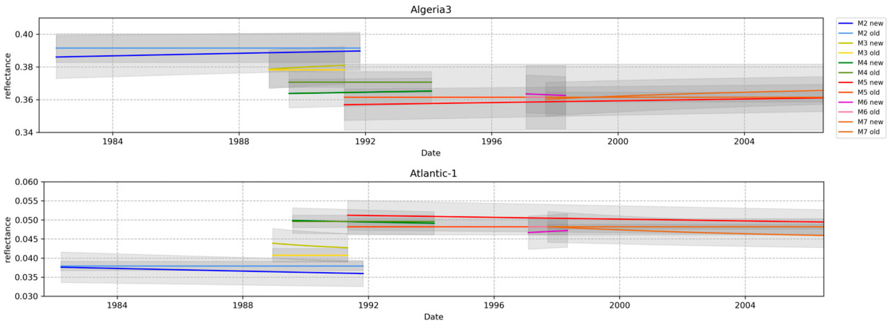
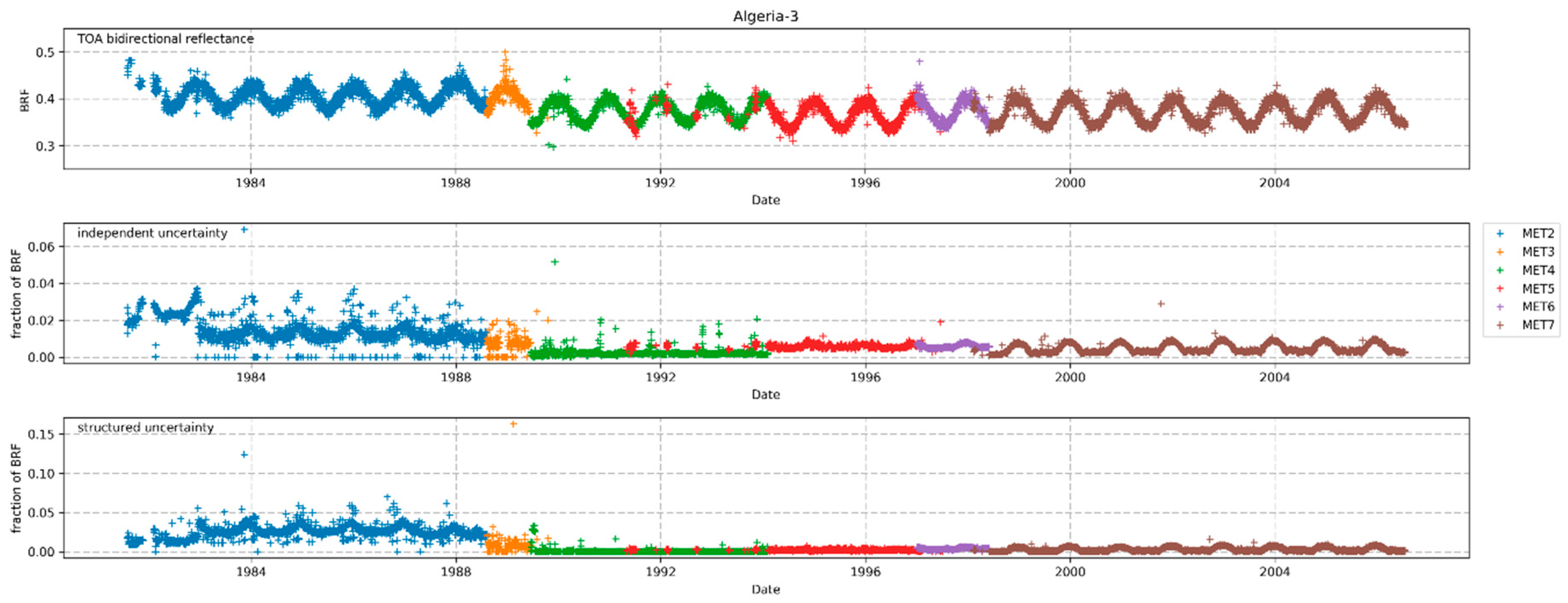
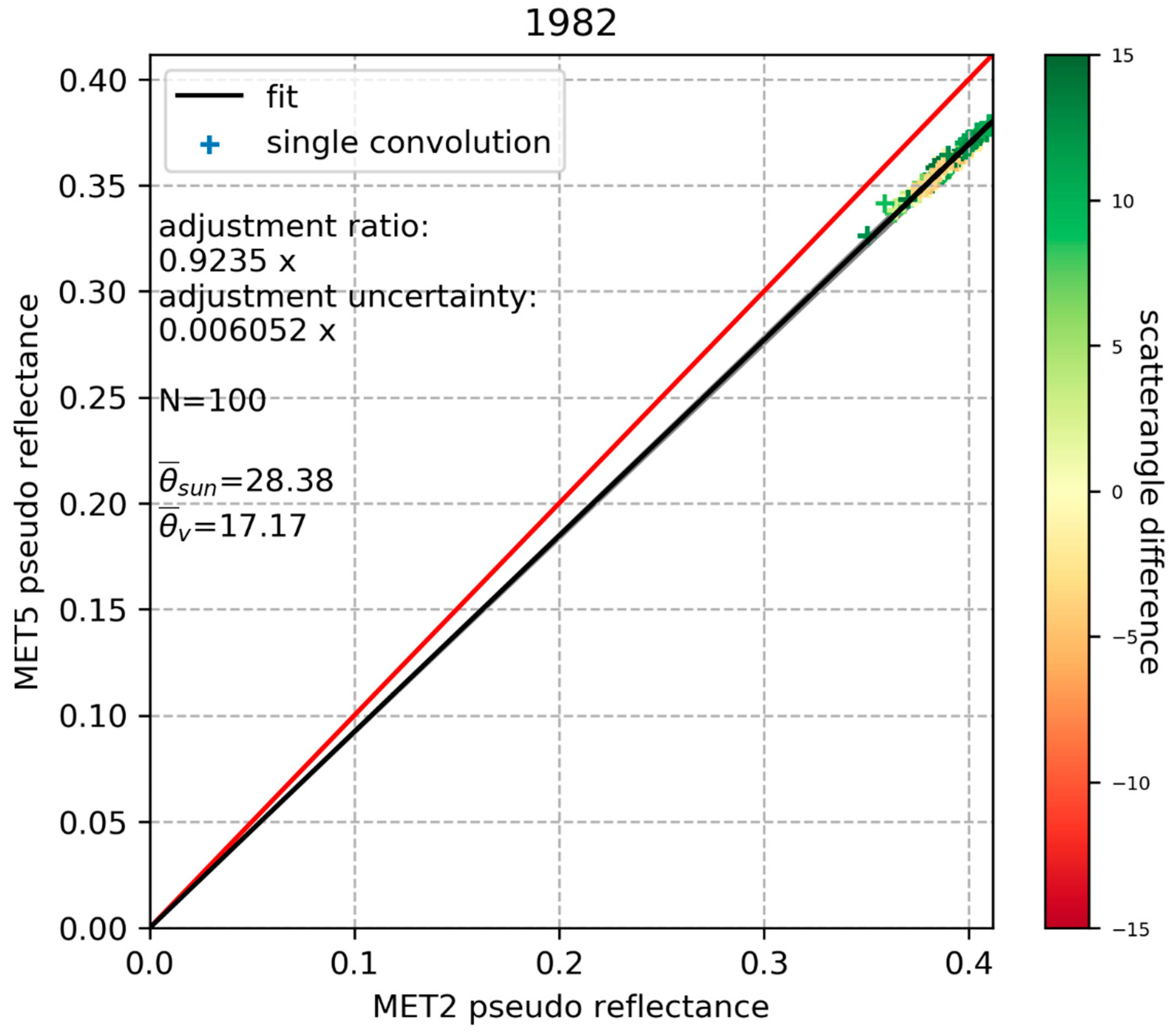
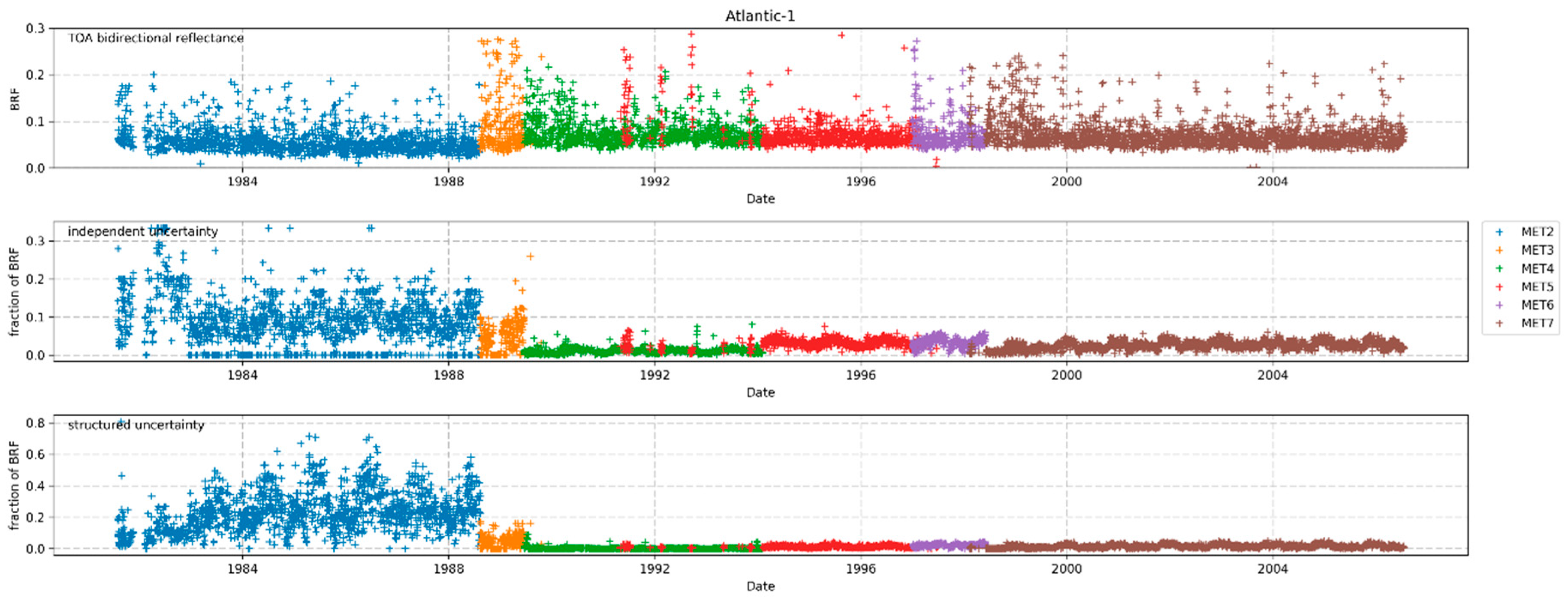
Using the new SRFs, using the same calibration reference targets, and applying the same methodology for all instruments have resulted in the production of a harmonised time-series of MVIRI visible channel measurements. As discussed in the paper, this harmonised time-series retains spectral differences between different instruments, but reduces uncertainties caused by, for example, the use of imprecise spatial, temporal and angular information. In the harmonised dataset a blue target, for example, will appear darker in Meteosat-2 than in Meteosat-7 due to the higher spectral response in the blue part of the spectrum for Meteosat-7.

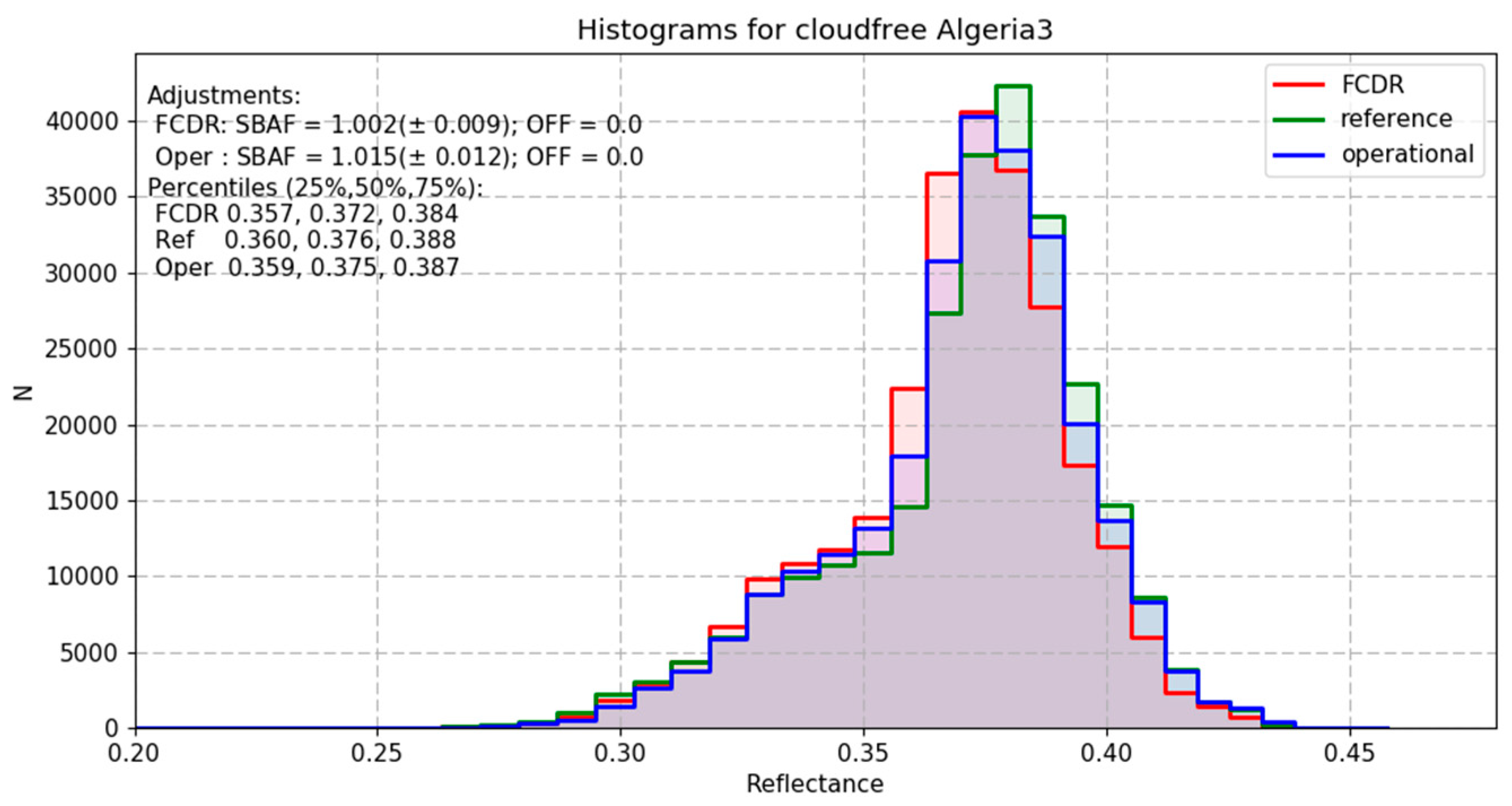
In order to remove differences caused by such spectral signatures, a harmonised FCDR needs to be homogenised. Therefore, the SRF of each sensor in the time-series is adjusted to the SRF of a baseline sensor. This adjustment has to be done for each target separately. In this paper the homogenisation is performed by using spectra observed by SCIAMACHY. It is shown that the time-series of the homogenised FCDR is stable from instrument to instrument over a selected number of targets. Only at the Atlantic-1 target-site some remaining mismatch is identified pointing to an overestimation of the Meteosat-2 SRF in the blue part of the spectrum. Despite the successful homogenisation for the selected target-sites, it has to be pointed out that an a-priory homogenisation of the entire FCDR is impossible to provide, due to the spatiotemporal variability in the spectral signature of the observed scenes. Users of harmonised data records need to be aware of the inter-instrumental differences due to differences in the SRFs. The authors strongly recommend the use of the harmonised MVIRI FCDR which may improve retrievals or assimilation systems that correctly take into account temporal variations in the reconstructed SRFs.

The paper describes the methods used for rigorously tracing the uncertainty of different physical effects for the precision and trueness of the measurements. The resulting pixel-level uncertainties have been analysed along with information about the spatiotemporal correlation properties of the underlying errors. In the methods section it is shown that it is possible to combine different effects into independent and structured uncertainties. Those uncertainties allow the proper quantification of the uncertainties resulting from, for example, the changing resolution of the dynamic range (6 bit to 8 bit), the different noise levels of the detectors, or the remaining uncertainties of the recalibration process. Not yet included in the uncertainty analysis of the FCDR is an uncertainty of the solar spectrum. As the same solar spectrum is used for the calibration and for the reflectance computation, the impact on the uncertainty budged is assumed to largely cancel out. However, a future release of the dataset should include a proper quantification of this effect. The same holds true for a revision of the assumption of entirely uncorrelated errors of the modelled atmosphere that is used for the vicarious calibration (Table 3).

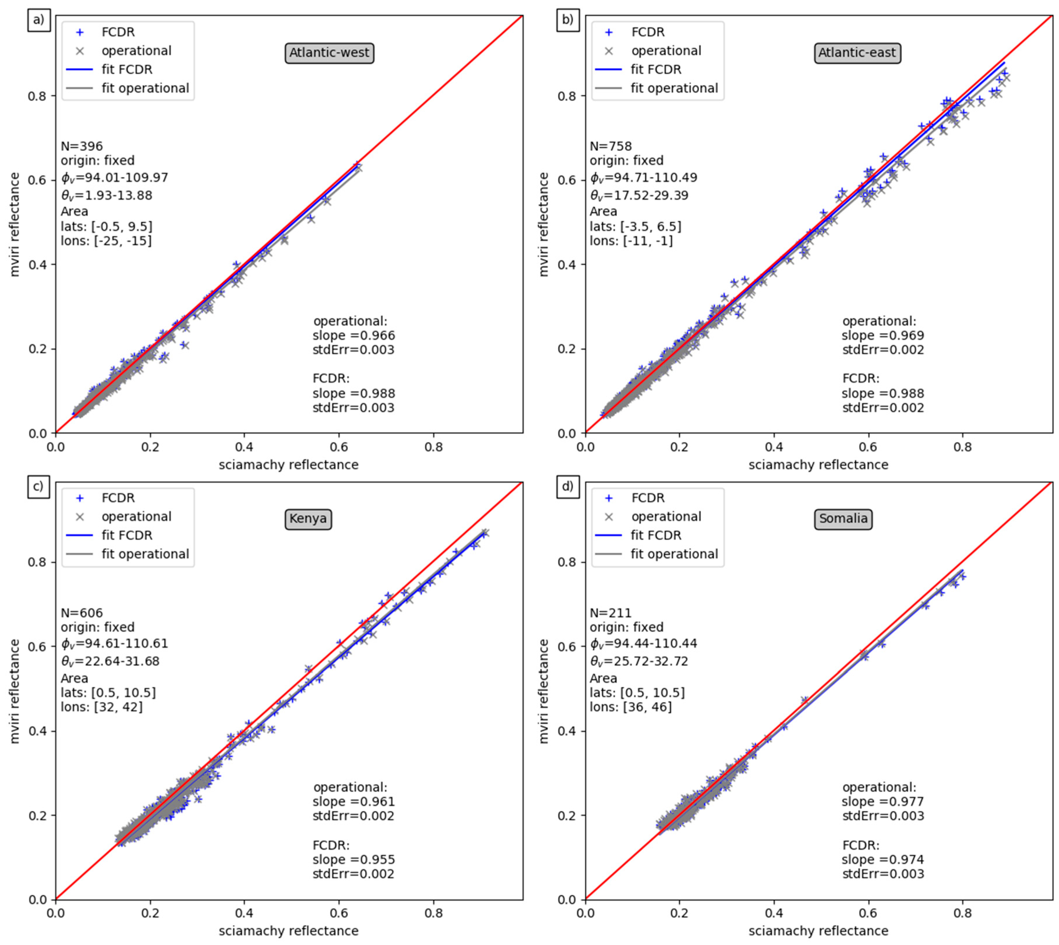
In a thorough validation against data from the SEVIRI instrument onboard MSG and against collocated and ray-matched measurements from SCIAMACHY the improved trueness of the dataset over cloudy and ocean areas is demonstrated. Over cloudy areas, the harmonised MVIRI FCDR is brighter than the operational MVIRI data record, which results in a better match with the SEVIRI cloud reflectances. The brighter reflectance values for high-clouds, for example, are estimated to affect the top of atmosphere outgoing shortwave radiation by about 8 W/m². The difference between the harmonised MVIRI FCDR and the operational MVIRI data record is small over areas with dominant spectral contributions in the green and red part of the spectrum. The analysis of SNOs between the harmonised MVIRI FCDR and SCIAMACHY has revealed excellent agreement with slopes close to unity (~0.98 over ocean areas and ~0.96 over land areas).

The data record described in this paper can be ordered via the EUMETSAT User Service Helpdesk in Darmstadt, Germany. Please send a written request to [email protected], indicating whether you want to order the normal FCDR (easy-FCDR) or the extended (full-FCDR) version.

References

1. Govaerts, Y.M.; Luffarelli, M. Joint retrieval of surface reflectance and aerosol properties with continuous variation of the state variables in the solution space—Part 1: Theoretical concept. Atmos. Meas. Tech. 2018, 11, 6589–6603. [Google Scholar] [CrossRef]
2. Stöckli, R.; Bojanowski, J.S.; John, V.O.; Duguay-Tetzlaff, A.; Bourgeois, Q.; Schulz, J.; Hollmann, R. Cloud Detection with Historical Geostationary Satellite Sensors for Climate Applications. Remote Sens. 2019, 11, 1052. [Google Scholar] [CrossRef]
3. Govaerts, Y.M. Correction of the Meteosat-5 and -6 radiometer solar channel spectral response with the Meteosat-7 sensor spectral characteristics. Int. J. Remote Sens. 1999, 10, 3677–3682. [Google Scholar] [CrossRef]
4. Decoster, I.; Govaerts, Y.M.; Baudrez, E.; Dewitte, S.; Velazquez, A.; Blazquez, A.; Cornelis, J. Evidence of pre-launch characterization problem of Meteosat-7 visible spectral response. Remote Sens. Lett. 2013, 4, 1008–1017. [Google Scholar] [CrossRef]
5. Decoster, I.; Clerbaux, N.; Baudrez, E.; Dewitte, S.; Ipe, A.; Nevens, S.; Blazquez, A.V.; Cornelis, J. A Spectral Ageing Model for the Meteosat-7 Visible Band. J. Atmos. Ocean. Technol. 2013, 30, 496–509. [Google Scholar] [CrossRef]
6. Decoster, I.; Clerbaux, N.; Baudrez, E.; Dewitte, S.; Ipe, A.; Nevens, S.; Blazquez, A.; Cornelis, J. Spectral Aging Model Applied to Meteosat First Generation Visible Band. Remote Sens. 2014, 6, 2534–2571. [Google Scholar] [CrossRef]
7. Meirink, J.F.; Roebeling, R.A.; Stammes, P. Inter-calibration of polar imager solar channels using SEVIRI. Atmos. Meas. Tech. 2013, 6, 2495–2508. [Google Scholar] [CrossRef]
8. Govaerts, Y.M.; Arriaga, A.; Schmetz, J. Operational vicarious calibration of the MSG/SEVIRI solar channels. Adv. Space Res. 2001, 28, 21–30. [Google Scholar] [CrossRef]
9. Goldberg, M.; Ohring, G.; Butler, J.; Cao, C.; Datla, R.; Doelling, D.; Gaertner, V.; Hewison, T.; Iacovazzi, B.; Kim, D.; et al. The global space-based inter-calibration system (GSICS). Bull. Am. Meteorol. Soc. 2011, 92, 468–475. [Google Scholar] [CrossRef]
10. Stone, T.C.; Rossow, W.B.; Ferrier, J.; Hinkelman, L.M. Evaluation of ISCCP Multisatellite Radiance Calibration for Geostationary Imager Visible Channels Using the Moon. IEEE Trans. Geosci. Remote Sens. 2008, 51, 1255–1266. [Google Scholar] [CrossRef]
11. Chander, G.; Hewison, T.J.; Fox, N.; Wu, X.; Xiong, X.; Blackwell, W.J. Overview of intercalibration of satellite instruments. IEEE Trans. Geosci. Remote Sens. 2013, 51, 1056–1080. [Google Scholar] [CrossRef]
12. Xiong, X.; Chiang, K.; Esposito, J.; Guenther, B.; Barnes, W. MODIS on-orbit calibration and characterization. Metrologia 2003, 40, S89–S92. [Google Scholar] [CrossRef]
13. Choi, T.; Shao, X.; Cao, C.; Weng, F. Radiometric Stability Monitoring of the Suomi NPP Visible Infrared Imaging Radiometer Suite (VIIRS) Reflective Solar Bands Using the Moon. Remote Sens. 2016, 8, 15. [Google Scholar] [CrossRef]
14. Arriaga, A.; Schmetz, J. Calibration of the Meteosat-5/-6 VIS channels with help of modelled radiances. Contrib. Atmos. Phys. 1999, 72, 133–139. [Google Scholar]
15. Doelling, D.R.; Morstad, D.; Bhatt, R.; Scarino, B. Algorithm Theoretical Basis Document (ATBD) for Deep Convective Cloud (DCC) Technique of Calibrating GEO Sensors with Aqua-MODIS for GSICS. GSICS, 2011. Available online: http://gsics.atmos.umd.edu/pub/Development/AtbdCentral/GSICS_ATBD_DCC_NASA_2011_09.pdf (accessed on 14 May 2019).
16. Wielicki, B.A.; Young, D.F.; Mlynczak, M.G. Achieving Climate Change Absolute Accuracy in Orbit. Bull. Am. Meteor. Soc. 2013, 94, 1519–1539. [Google Scholar] [CrossRef]
17. Doelling, D.R.; Lukashin, C.; Minnis, P.; Scarino, B.; Morstad, D. Spectral reflectance corrections for satellite intercalibrations using SCIAMACHY data. IEEE Geosci. Remote Sens. Lett. 2012, 9, 119–123. [Google Scholar] [CrossRef]
18. Roebeling, R.A.; Deneke, H.M.; Feijt, A.J. Validation of cloud liquid water path retrievals from SEVIRI using one year of CLOUDNET observations. J. Appl. Meteorol. Climatol. 2008, 1, 47. [Google Scholar] [CrossRef]
19. Doelling, D.R.; Scarino, B.R.; Morstad, D.; Gopalan, A.; Bhatt, R.; Lukashin, C.; Minnis, P. The Intercalibration of Geostationary Visible Imagers Using Operational Hyperspectral SCIAMACHY Radiances. IEEE Trans. Geosci. Remote Sens. 2013, 51, 1245–1254. [Google Scholar] [CrossRef]
20. Mittaz, J.; Merchant, C.J.; Wooliams, E. Applying principles of metrology to historical Earth observations from satellites. Metrologia 2019, accepted. [Google Scholar] [CrossRef]
21. Govaerts, Y.; Rüthrich, F.; John, V.; Quast, R. Climate Data Records from Meteosat First Generation Part I: Simulation of Accurate Top-Of-Atmosphere Spectral Radiance over Pseudo-Invariant Calibration Sites for the Retrieval of the in-flight MVIRI/VIS Spectral Response. Remote Sens. 2018, 10, 1959. [Google Scholar] [CrossRef]
22. Quast, R.; Giering, R.; Govaerts, Y.; Rüthrich, F.; Roebeling, R. Climate Data Records from Meteosat First Generation Part II: Retrieval of the In-Flight VIS Spectral Response. Remote Sens. 2019, 11, 480. [Google Scholar] [CrossRef]
23. Giering, R.; Quast, R.; Hunt, S.; Harris, P.; Mittaz, J.; Wooliams, E. Harmonisation of Satellite Sensors. Remote Sens. 2019, 11, 1002. [Google Scholar] [CrossRef]
24. John, V.O.; Tabata, T.; Rüthrich, F.; Roebeling, R.; Hewison, T.; Stöckli, R.; Schulz, J. On the Methods for Recalibrating Geostationary Longwave Channels Using Polar Orbiting Infrared Sounders. Remote Sens. 2019, 11, 1171. [Google Scholar] [CrossRef]
25. Wolff, T. An image geometry model for METEOSAT. Int. J. Remote Sens. 1985, 6, 1599–1606. [Google Scholar] [CrossRef]
26. Keys, R.G. Cubic Convolution Interpolation for Digital Image Processing. IEEE Trans. Acoust. Speech Signal Process. 1981, 29, 1153–1160. [Google Scholar] [CrossRef]
27. Govaerts, Y.; Clerici, M. MSG-1/SEVIRI Solar Channels Calibration Commissioning Activity Report. 2004. Available online: https://www.eumetsat.int/website/home/Data/Products/Calibration/MSGCalibration (accessed on 31 January 2019).
28. Lichtenberg, G.; Kleipool, Q.; Krijger, J.M.; van Soest, G.; van Hees, R.; Tilstra, L.G.; Acarreta, J.R.; Aben, I.; Ahlers, B.; Bovensmann, H.; et al. SCIAMACHY Level 1 data: Calibration concept and in-flight calibration. Atmos. Chem. Phys. 2006, 6, 5347–5367. [Google Scholar] [CrossRef]
29. SCIAMACHY Product Handbook. 2013. Available online: https://earth.esa.int/web/guest/missions/esa-operational-eo-missions/envisat/instruments/sciamachy-handbook/wiki (accessed on 31 January 2019).
30. Tilstra, L.G.; Tuinder, O.N.E.; Wang, P.; Stammes, P. Surface reflectivity climatologies from UV to NIR determined from Earth observations by GOME-2 and SCIAMACHY. J. Geophys. Res. Atmos. 2017, 122, 4084–4111. [Google Scholar] [CrossRef]
31. Burrows, J.P.; Goede, A.P.H.; Muller, C.; Bovensmann, H. SCIAMACHY—The Need for Atmospheric Research from Space. In SCIAMACHY-Exploring the Changing Earth’s Atmosphere; Gottwaldand, M., Bovensmann, H., Eds.; Springer: Dordrecht, The Netherlands, 2011. [Google Scholar] [CrossRef]
32. Doelling, D.R.; Haney, C.O.; Scarino, B.R.; Gopalan, A.; Bhatt, R. Improvements to the geostationary visible imager ray-matching calibration algorithm for CERES Edition 4. J. Atmos. Ocean. Technol. 2016, 33, 2679–2698. [Google Scholar] [CrossRef]
33. Roebeling, R.A.; Feijt, A.J.; Stammes, P. Cloud property retrievals for climate monitoring: Implications of differences between Spinning Enhanced Visible and Infrared Imager (SEVIRI) on METEOSAT-8 and Advanced Very High Resolution Radiometer (AVHRR) on NOAA-17. J. Geophys. Res. 2006, 111, D20210. [Google Scholar] [CrossRef]
34. Musial, J.P.; Bojanowski, J.S. AVHRR LAC satellite cloud climatology over Central Europe derived by the Vectorized Earth Observation Retrieval (VEOR) method and PyLAC software. Geoinf. Issues 2017, 9, 39–51. [Google Scholar]
35. Snel, R.; Lichtenberg, G.; Noël, S.; Krijger, M.; Slijkhuis, K.; Bramstedt, K. Calibration and Monitoring. In SCIAMACHY-Exploring the Changing Earth’s Atmosphere; Gottwaldand, M., Bovensmann, H., Eds.; Springer: Dordrecht, The Netherlands, 2011. [Google Scholar] [CrossRef]
36. SCIAMACHY L1c Command-line Tool Landing Pages. Available online: https://earth.esa.int/web/guest/software-tools/content/-/article/scial1c-command-line-tool-4073 (accessed on 1 February 2019).
37. Nicodemus, F.E.; Richmond, J.C.; Hsia, J.J.; Ginsberg, I.W.; Limperis, T. Geometrical Considerations and Nomenclature for Reflectance; National Bureau of Standards; U.S. Governement Printing Office: Washington, DC, USA, 1977.
38. Rüthrich, F.; John, V.O.; Roebeling, R.; Wagner, S.; Viticchie, B.; Hewison, T.; Govaerts, Y.; Quast, R.; Giering, R.; Schulz, J. A Fundamental Climate Data Record that accounts for Meteosat First Generation Visible Band Spectral Response Issues. In Proceedings of the 2016 EUMETSAT Meteorological Satellite Conference, Darmstadt, Germany, 26–30 September 2016. [Google Scholar]
39. Mittaz, J. Instrument Noise Characterization and the Allan/M-Sample. 2016. Available online: http://www.fiduceo.eu/sites/default/files/publications/noise_and_allan_variance_report.pdf (accessed on 14 February 2019).
40. BIPM. Evaluation of Measurement Data—Guide to the Expression of the Uncertainty in Measurement; Technical Report JCGM 100:2008 GUM 1995 with minor corrections; BIPM: Cedex, France, 2008. [Google Scholar]
Figure 1. The MVIRI uncertainty diagram illustrates the effects that contribute to the uncertainties of the different parameters of the measurement equation. Note that the measurement equation here is Equation (1) where the calibration coefficient a c f is expanded by Equation (10). Notation is explained in the text.
Remotesensing 11 01165 g001
Figure 2. Spectral Response functions of Meteosat-2-7 plotted together with SCanning Imaging Absorption spectroMeter for Atmospheric CartograpHY (SCIAMACHY) spectra acquired during 2002 at three target sites. (a) shows the spectra measured by SCIAMACHY at the Algeria site, (b) shows the spectra measured at the Nile-delta and the (c) shows those measured at the Atlantic-1 site. Spectra are plotted at in transparent black to better illustrate their spread. Spectra with strong cloud contamination were removed before plotting (see Section 3.9.1). Note that for band-adjustment/homogenisation more sophisticated filtering regarding clouds and scene heterogeneity is applied (Section 3.9.1).
Remotesensing 11 01165 g002
Figure 3. Scan pattern of one SCIAMACHY overpass over Algeria-3 with 4 pixel per scanline. The numbers provide the viewing zenith angle at the center of each pixel. The green box is the 2° × 2° box of the target site. The red pixel are considered for the computation of the spectral band adjustment factor for the homogenisation of the timeseries at this target. The orange pixel are disregarded.
Remotesensing 11 01165 g003
Figure 4. Mean SCIAMACHY spectrum collected above the Algeria-3 validation site along with the spectral response functions of the VIS channel on Meteosat-7 and the HRVIS channel on MSG1.
Remotesensing 11 01165 g004
Figure 5. Convoluted clear-sky SCIAMACHY spectra above Algeria-3 using Meteosat-2 and Meteosat-5 SRFs that were valid at each satellites’ launch date.
Remotesensing 11 01165 g005
Figure 6. Illustration of the approach for the MVIRI/SEVIRI comparison. Site-specific spectral band adjustment functions between the two MVIRI datasets and the SEVIRI HRVIS band are computed based on SCIAMACHY spectra that are collected during a five-month period. The five-month period envelops the one-month period during which the actual MVIRI and SEVIRI data are collected that are displayed in the histograms.
Remotesensing 11 01165 g006
Figure 7. Locations of the areas considered for finding potentially ray-matched SCIAMACHY-MVIRI collocations (Zero Degree Mission (ZDM) and Indian Ocean data coverage (IODC)) that are exploited in this study. The collocation results for each area are presented in Figure 16.
Remotesensing 11 01165 g007
Figure 8. Expected time series at Algeria-3 and Atlantic-1 based on representative mean SCIAMACHY spectra (Figure 2) that are convoluted with the pre-launch SRFs (old) and with the time-variant, reconstructed SRFs (new). Grey shading is the uncertainty of the reflectance computed from the uncertainty provided along with the SRFs.
Remotesensing 11 01165 g008
Figure 9. Harmonised MVIRI VIS fundamental climate data records (FCDR) time series of clear-sky reflectance at Algeria-3 along with structured and independent uncertainties. Trends and jumps are due to the changing SRFs. Alternating measurements from two satellites, as in 1992, are mostly due to a takeover by the backup satellite during maintenance operations of the primary satellite.
Remotesensing 11 01165 g009
Figure 10. Harmonised MVIRI VIS FCDR time series of clear-sky reflectance at Atlantic-1 along with structured and independent uncertainties. Trends and jumps are due to the changing SRFs. Alternating measurements from two satellites, as in 1992, are mostly due to a takeover by the backup satellite during maintenance operations of the primary satellite.
Remotesensing 11 01165 g010
Figure 11. Homogenised time series of recalibrated broadband reflectances at Algeria-3, Nile-delta and Atlantic-1.
Remotesensing 11 01165 g011
Figure 12. Anomalies of the homogenised reflectance time series and their trends. Anomalies are the deviation from the mean annual reflectance cycles. Additional filtering for cloud contamination was applied. The filter computes the 25th percentile from a rolling kernel of 30 days around each reflectance measurement. Measurements that are brighter than this value are rejected in order to display only measurements that are certainly cloud free. Note that for the Atlantic site the periods with globally elevated aerosol loads due to volcanic eruptions are excluded from the stability analysis.
Remotesensing 11 01165 g012
Figure 13. Histogram of SEVIRI HRVIS plotted as reference together with the histograms of the operational MVIRI dataset and the recalibrated MVIRI FCDR, as obtained from cloud-free Algeria-3 pixels at 12:00 UTC slots during March 2005. The MVIRI datasets are band adjusted to the SRF of the SEVIRI HRVIS band according to the given Spectral Band Adjustment Factors (SBAFs). The SBAFs are computed on the same set of SCIAMACHY spectra and the difference between both SBAFs is entirely due to the different shapes of the SRFs in the operational and the FCDR dataset.
Remotesensing 11 01165 g013
Figure 14. Histogram of SEVIRI HRVIS plotted as reference together with the histograms of the operational MVIRI dataset and the recalibrated MVIRI FCDR, as obtained from entirely cloud-covered pixels at 12:00 UTC slots during March 2005. Clouds are classified into high clouds (a), middle clouds (b) and low clouds (c). The MVIRI datasets were band adjusted to the SRF of the SEVIRI HRVIS band according to the given SBAFs. For each cloud-class the SBAFs for the operational dataset and for the FCDR are computed on the same set of SCIAMACHY spectra and the difference between both SBAFs is entirely due to the different shapes of the SRFs in the operational dataset and the FCDR.
Remotesensing 11 01165 g014
Figure 15. Histogram of SEVIRI HRVIS plotted as reference together with the histograms of the operational MVIRI dataset and the recalibrated MVIRI FCDR, as obtained from cloud-free Atlantic-1 pixels at 12:00 UTC slots during March 2005. The MVIRI datasets were band adjusted to the SRF of the SEVIRI HRVIS band according to the given SBAFs. The SBAFs are computed on the same set of SCIAMACHY spectra and the difference between both SBAFs is entirely due to the different shapes of the SRFs in the operational and the FCDR dataset.
Remotesensing 11 01165 g015
Figure 16. Collocations between SCIAMACHY and MVIRI onboard MET7 for (a) Atlantic-west, (b) Atlantic-east and (c) Kenya. Collocations between SCIAMACHY and MET5 are provided in (d) for Somalia. Grey marks stand for the dataset with the pre-launch SRF characterisation. Blue crosses stand for the harmonised/recalibrated FCDR. The collocations are constrained to relative azimuth angles between the two instruments of 5°, to zenith angle differences of 15° and to acquisition time differences of 5 min. Only collocations with MVIRI standard deviation of below 0.12 within a SCIAMACHY pixel are considered. Over the Atlantic areas and the Somalian area collocations were acquired from data collected during 2002–2006, whereas data collected during 2006–2010 were used for the collocations over the Kenyan area.
Remotesensing 11 01165 g016
Figure 17. Spectral characteristics of the collocation regions and of Algeria-3 collected during 10 days of February 2005. In order to emphasise on cloud-free surfaces a set of 10% of the darkest spectra was averaged for each region. For the Atlantic site also a set of the 10% brightest spectra was averaged to illustrate the spectral shape of cloudy observations. The grey shading indicates the standard deviation of each set.
Remotesensing 11 01165 g017