Contribution of Land Surface Temperature (TCI) to Vegetation Health Index: A Comparative Study Using Clear Sky and All-Weather Climate Data Records


Abstract
1. Introduction
2. Materials and Methods
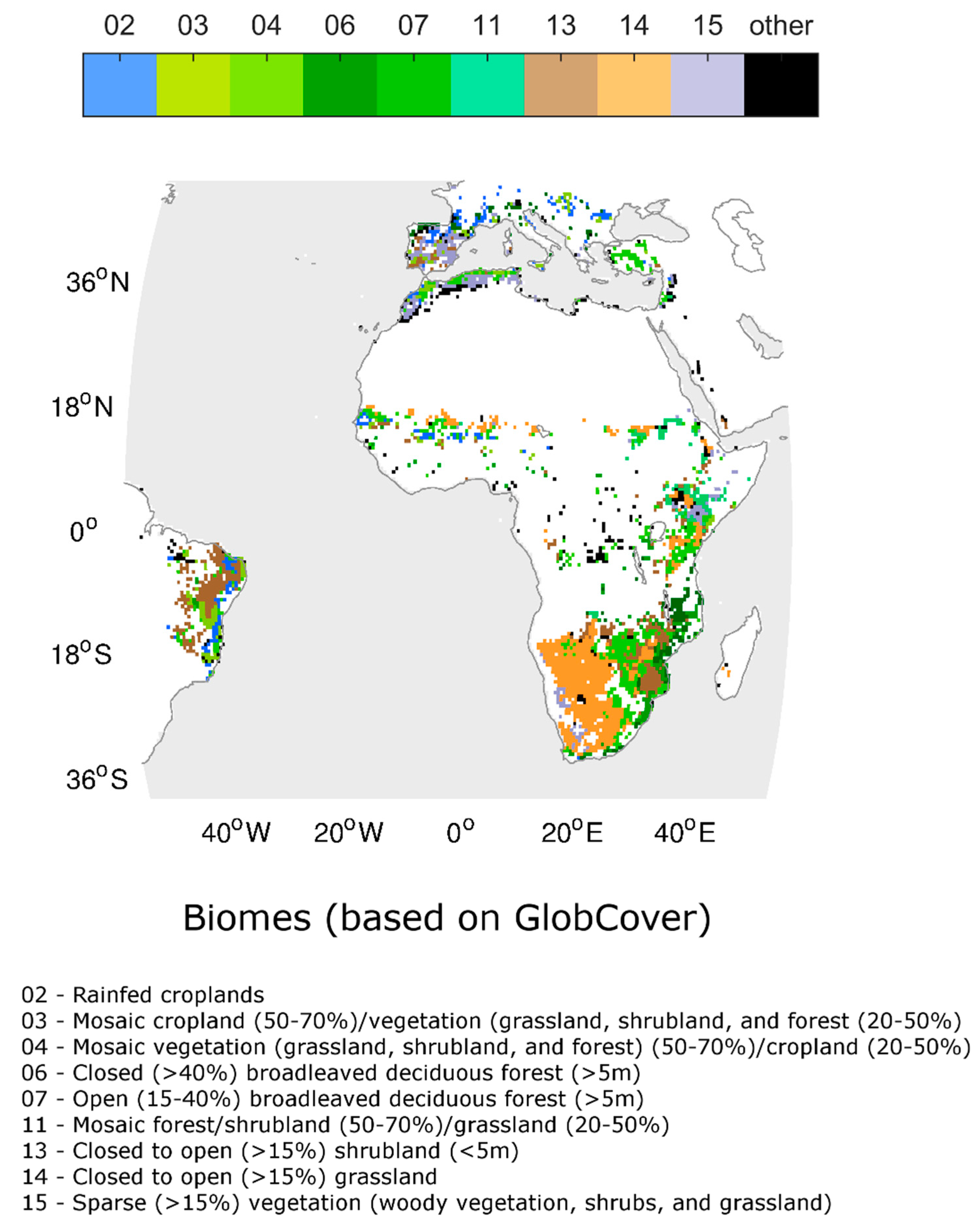
2.1. Study Area and Biome Classification
2.2. LST, NDVI Climate Data Records, and SPEI Dataset
2.3. Vegetation Health Index
2.4. Estimating Moisture (VCI) and Temperature (TCI) Contributions to VHI
3. Results
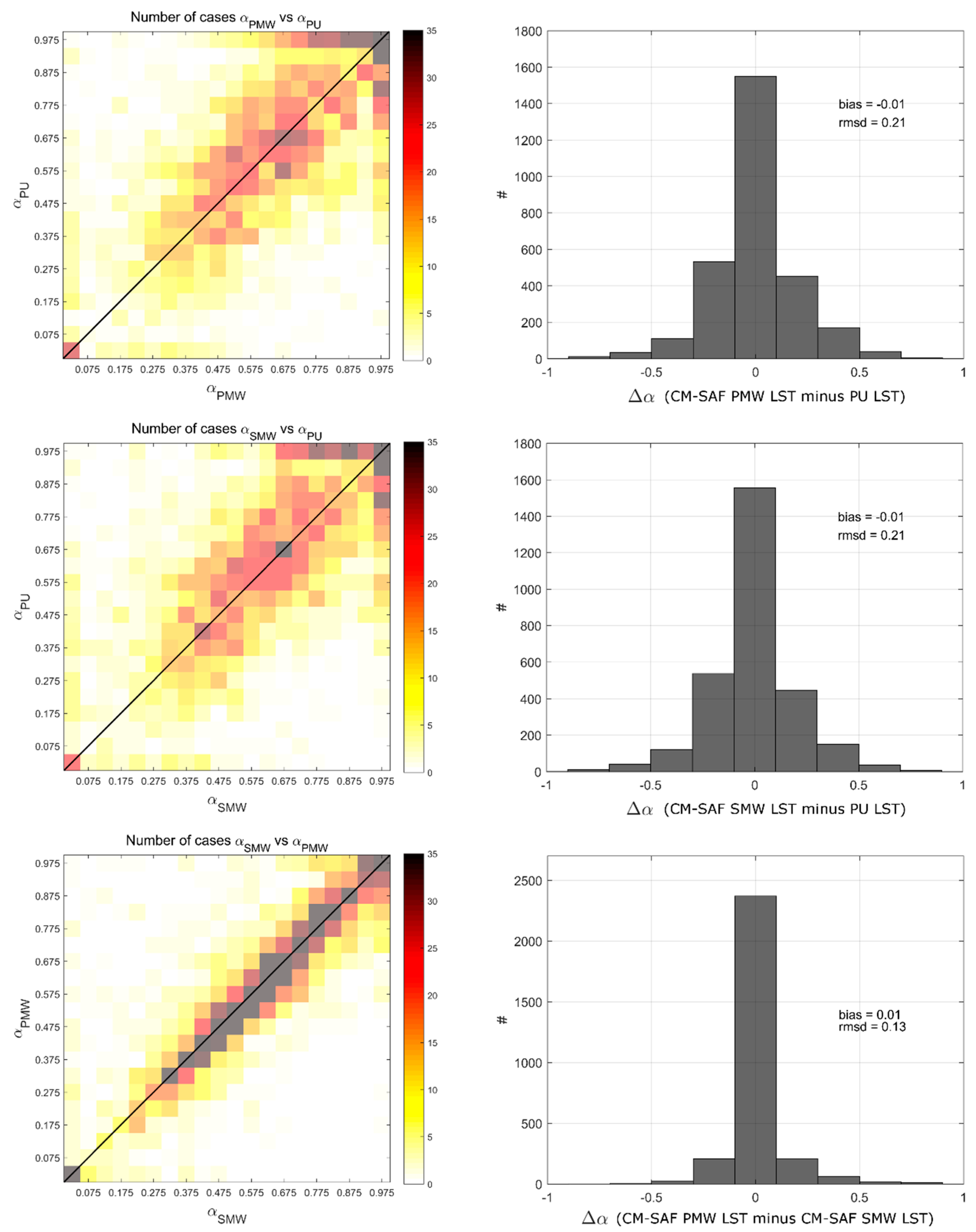
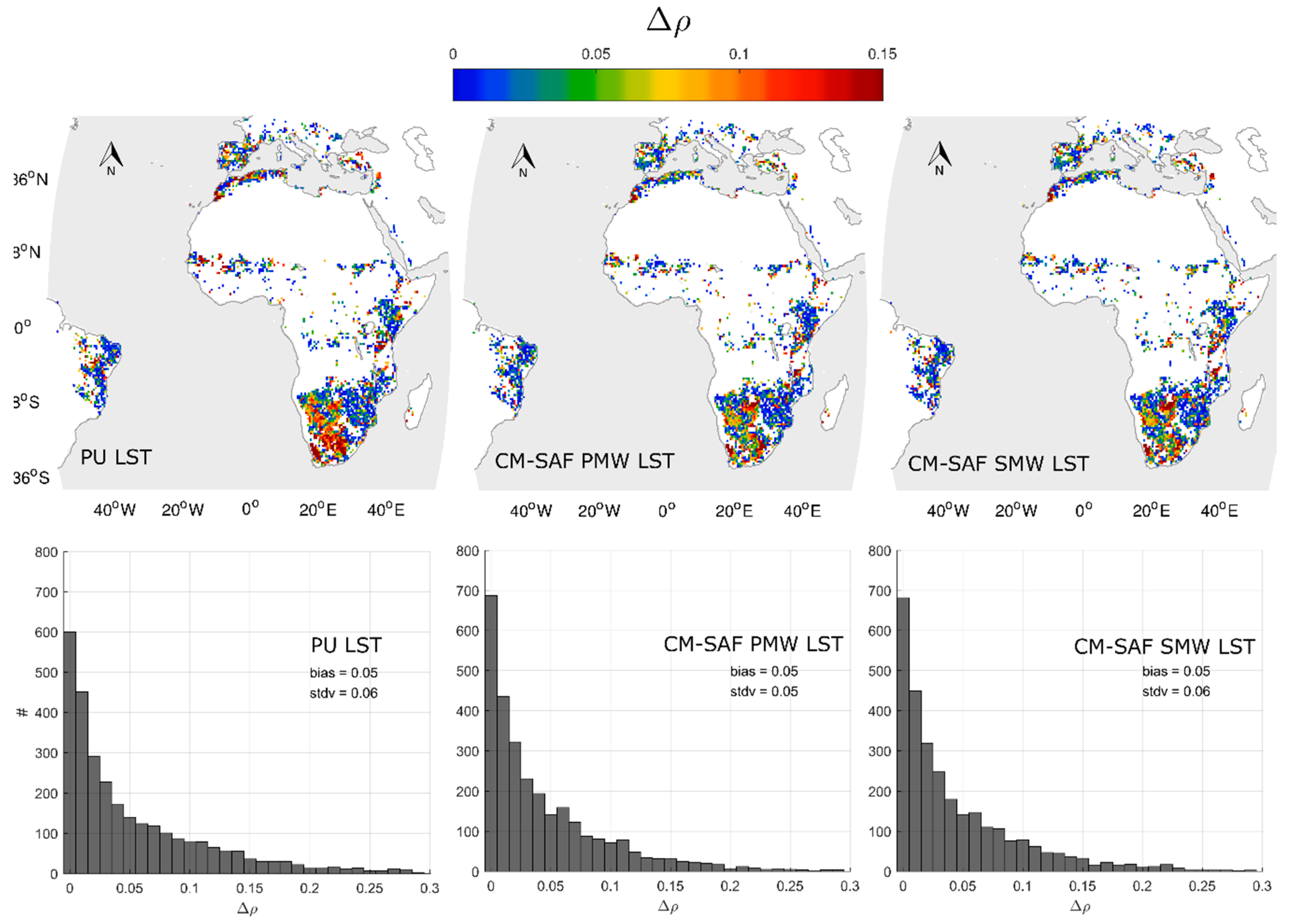
3.1. Comparison of Estimated with the Different LST CDRs
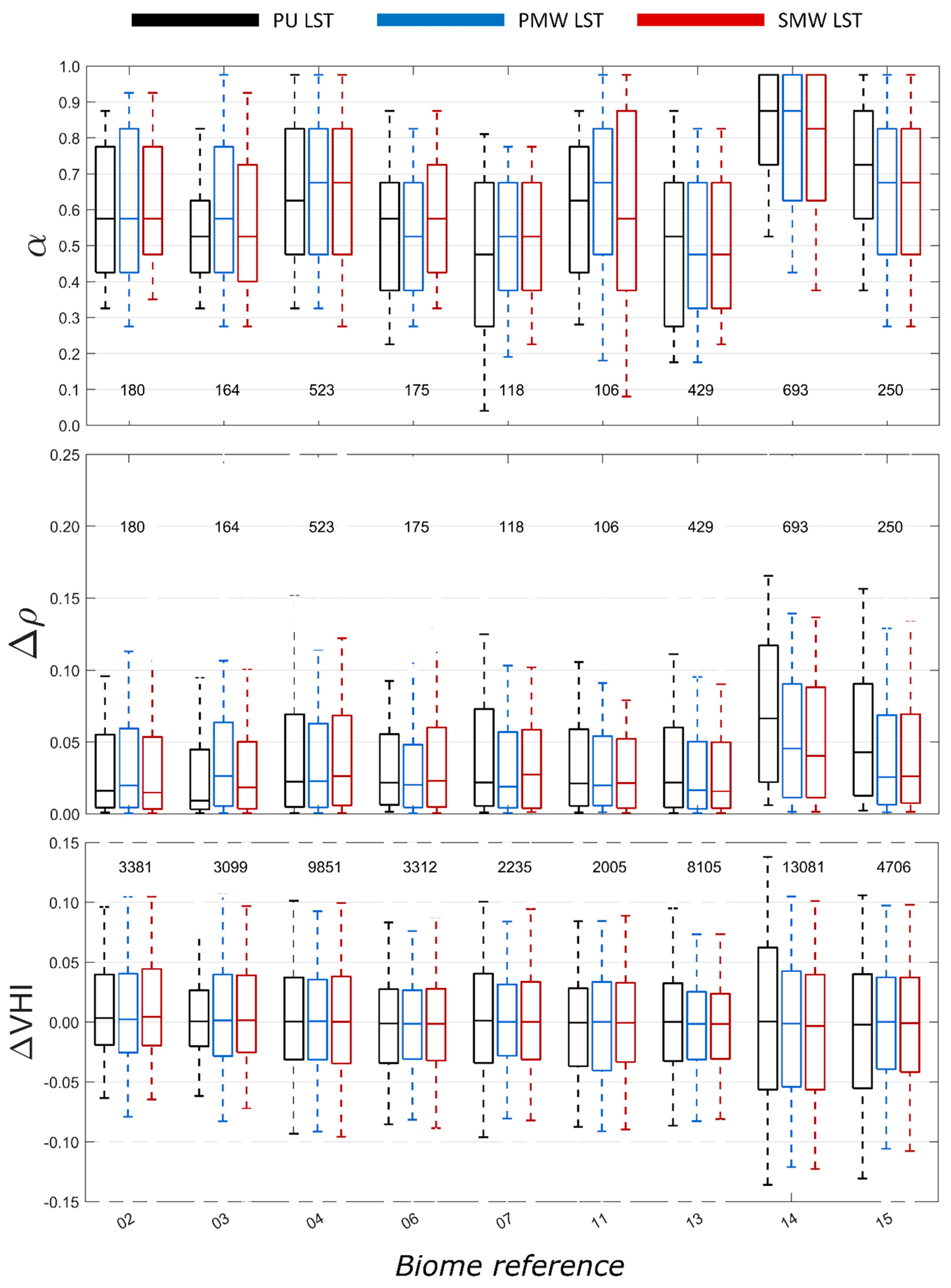
3.2. Biome Stratification
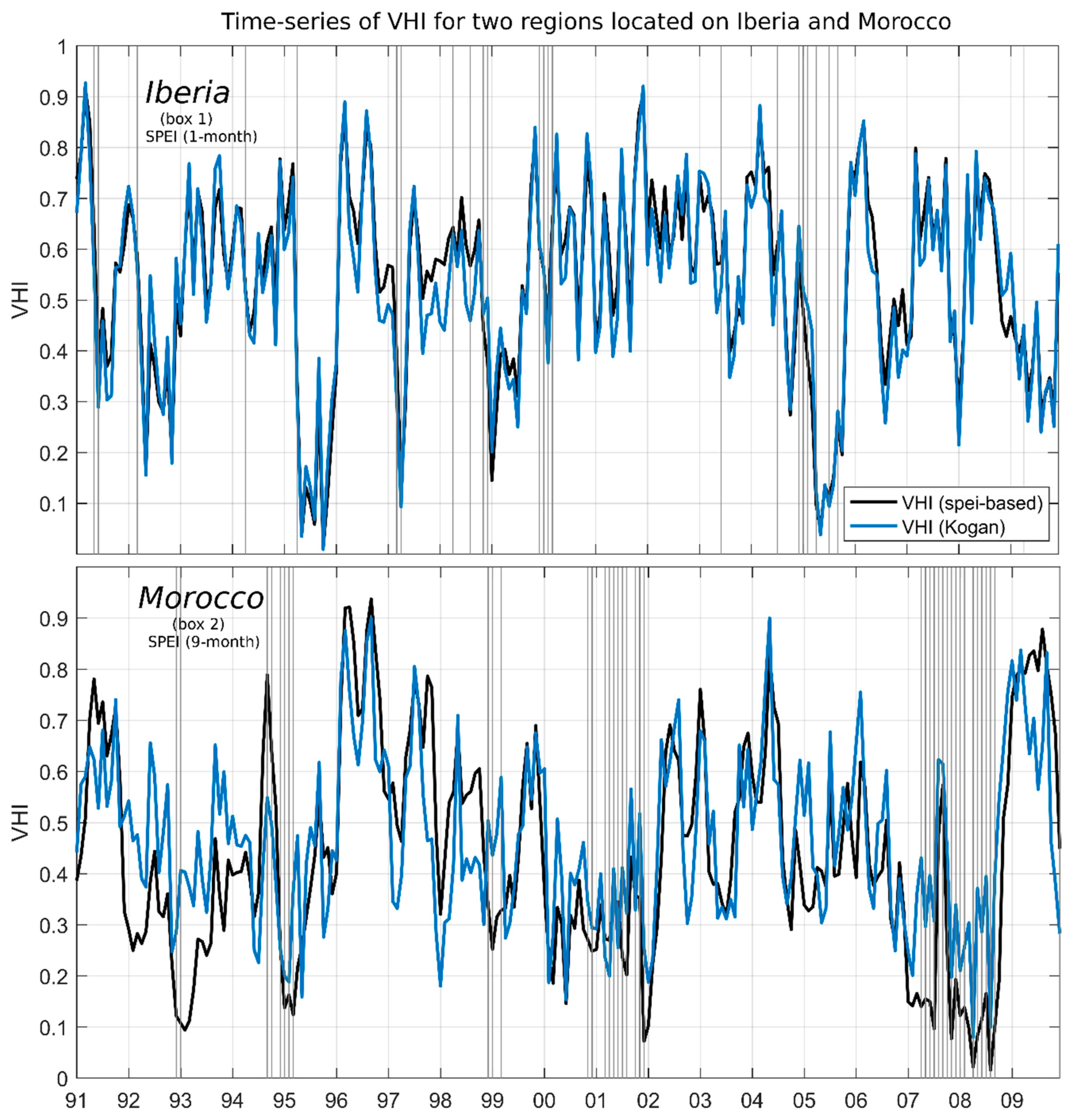
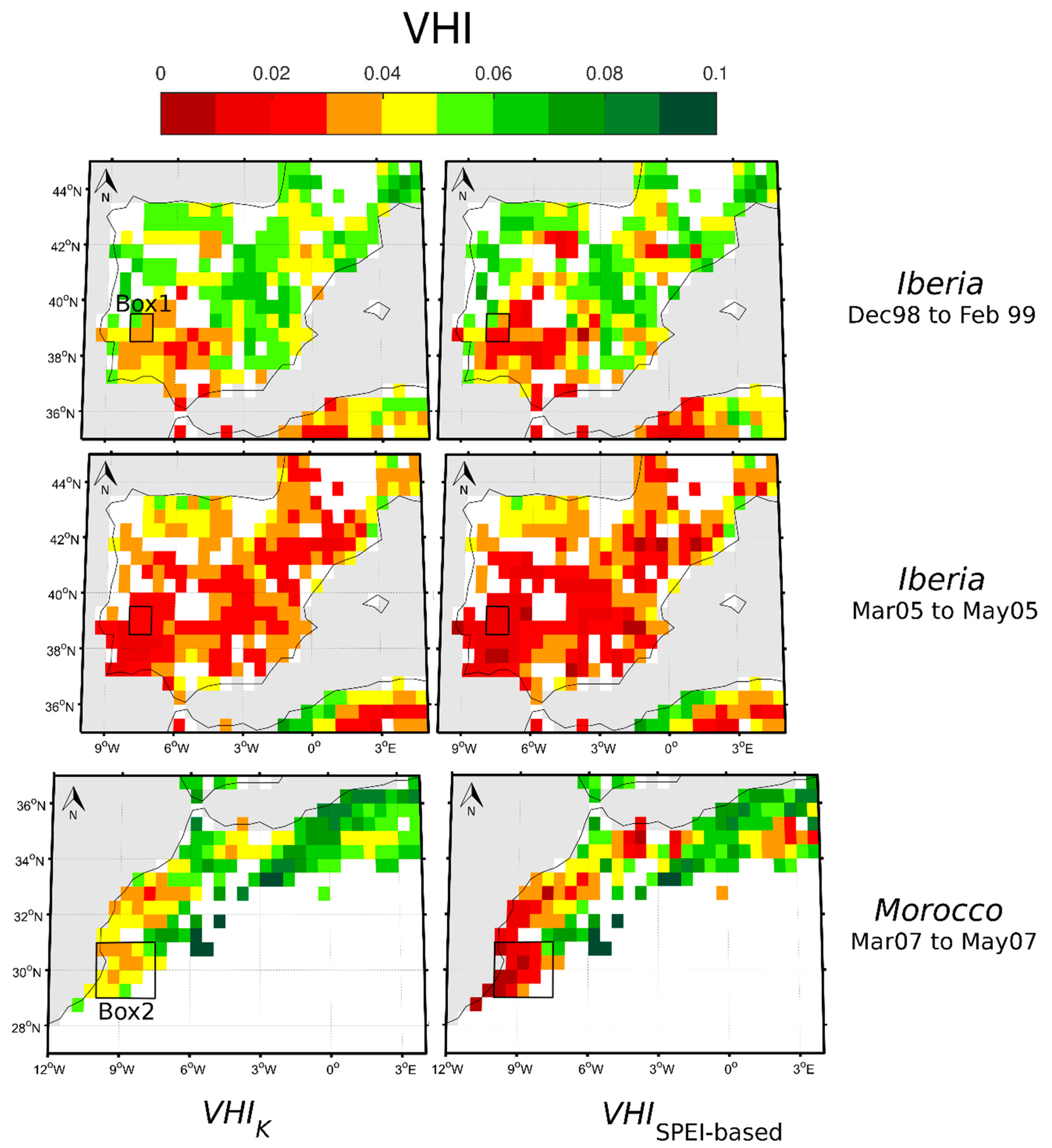
3.3. Comparison of VHI for Different Case Studies
4. Discussion
5. Conclusions
Author Contributions
Funding
Conflicts of Interest
References
- National Research Council. Climate Data Records from Environmental Satellites: Interim Report; The National Academies Press: Washington, DC, USA, 2004; ISBN 978-0-309-09168-8. [Google Scholar]
- Hollmann, R.; Merchant, C.J.; Saunders, R.; Downy, C.; Buchwitz, M.; Cazenave, A.; Chuvieco, E.; Defourny, P.; De Leeuw, G.; Forsberg, R.; et al. The ESA climate change initiative: Satellite data records for essential climate variables. Bull. Am. Meteorol. Soc. 2013, 94, 1541–1552. [Google Scholar] [CrossRef]
- Schulz, J.; Albert, P.; Behr, H.D.; Caprion, D.; Deneke, H.; Dewitte, S.; Dürr, B.; Fuchs, P.; Gratzki, A.; Hechler, P.; et al. Operational climate monitoring from space: The EUMETSAT satellite application facility on climate monitoring (CM-SAF). Atmos. Chem. Phys. 2009, 9, 1687–1709. [Google Scholar] [CrossRef]
- Plummer, S.; Lecomte, P.; Doherty, M. The ESA Climate Change Initiative (CCI): A European contribution to the generation of the Global Climate Observing System. Remote Sens. Environ. 2017, 203, 2–8. [Google Scholar] [CrossRef]
- Schröder, M.; Jonas, M.; Lindau, R.; Schulz, J.; Fennig, K. The CM SAF SSM/I-based total column water vapour climate data record: Methods and evaluation against re-analyses and satellite. Atmos. Meas. Tech. 2013, 6, 765–775. [Google Scholar] [CrossRef]
- Urbain, M.; Clerbaux, N.; Ipe, A.; Tornow, F.; Hollmann, R.; Baudrez, E.; Velazquez Blazquez, A.; Moreels, J. The CM SAF TOA Radiation Data Record Using MVIRI and SEVIRI. Remote Sens. 2017, 9, 466. [Google Scholar] [CrossRef]
- Merchant, C.J.; Embury, O.; Roberts-Jones, J.; Fiedler, E.; Bulgin, C.E.; Corlett, G.K.; Good, S.; McLaren, A.; Rayner, N.; Morak-Bozzo, S.; et al. Sea surface temperature datasets for climate applications from Phase 1 of the European Space Agency Climate Change Initiative (SST CCI). Geosci. Data J. 2014, 1, 179–191. [Google Scholar] [CrossRef]
- Song, Z.; Liang, S.; Wang, D.; Zhou, Y.; Jia, A. Long-term record of top-of-atmosphere albedo over land generated from AVHRR data. Remote Sens. Environ. 2018, 211, 71–88. [Google Scholar] [CrossRef]
- Lattanzio, A.; Fell, F.; Bennartz, R.; Trigo, I.F.; Schulz, J. Quality assessment and improvement of the EUMETSAT Meteosat Surface Albedo Climate Data Record. Atmos. Meas. Tech. 2015, 8, 4561–4571. [Google Scholar] [CrossRef]
- Duguay-Tetzlaff, A.; Bento, V.; Göttsche, F.M.; Stöckli, R.; Martins, J.; Trigo, I.F.; Olesen, F.; Bojanowski, J.; da Camara, C.; Kunz, H. Meteosat Land Surface Temperature Climate Data Record: Achievable Accuracy and Potential Uncertainties. Remote Sens. 2015, 7, 13139–13156. [Google Scholar] [CrossRef]
- Franch, B.; Vermote, E.F.; Roger, J.C.; Murphy, E.; Becker-reshef, I.; Justice, C.; Claverie, M.; Nagol, J.; Csiszar, I.; Meyer, D.; et al. A 30+ year AVHRR land surface reflectance climate data record and its application to wheat yield monitoring. Remote Sens. 2017, 9, 296. [Google Scholar] [CrossRef]
- Kim, Y.; Kimball, J.S.; Robinson, D.A.; Derksen, C. New satellite climate data records indicate strong coupling between recent frozen season changes and snow cover over high northern latitudes. Environ. Res. Lett. 2015, 10, 084004. [Google Scholar] [CrossRef]
- Bento, V.A.; Gouveia, C.M.; DaCamara, C.C.; Trigo, I.F. A climatological assessment of drought impact on vegetation health index. Agric. For. Meteorol. 2018, 259, 286–295. [Google Scholar] [CrossRef]
- Klos, R.J.; Wang, G.G.; Bauerle, W.L.; Rieck, J.R. Drought impact on forest growth and mortality in the southeast USA: An analysis using Forest Health and Monitoring data. Ecol. Appl. 2009, 19, 699–708. [Google Scholar] [CrossRef] [PubMed]
- Wilhite, D.A.; Svoboda, M.D.; Hayes, M.J. Understanding the complex impacts of drought: A key to enhancing drought mitigation and preparedness. Water Resour. Manag. 2007, 21, 763–774. [Google Scholar] [CrossRef]
- Hillier, D.; Dempsey, B. A Dangerous Delay: The Cost of Late Response to Early Warnings in the 2011 Drought in the Horn of Africa; Oxfam International Save the Children: Cowley, Oxford, UK, 2012; Volume 12, pp. 1–34. ISBN 978-1-78077-034-5. [Google Scholar]
- Ding, Y.; Hayes, M.J.; Widhalm, M. Measuring economic impacts of drought: A review and discussion. Disaster Prev. Manag. Int. J. 2011, 20, 434–446. [Google Scholar] [CrossRef]
- Mishra, A.K.; Singh, V.P. A review of drought concepts. J. Hydrol. 2010, 391, 202–216. [Google Scholar] [CrossRef]
- Zargar, A.; Sadiq, R.; Naser, B.; Khan, F.I. A review of drought indices. Environ. Rev. 2011, 19, 333–349. [Google Scholar] [CrossRef]
- Heim, R.R. Drought: A global assessment. In Drought Indices: A Review, 1st ed.; Routledge: London, UK, 2000; pp. 159–167. ISBN 0415168341. [Google Scholar]
- Palmer, W.C. Meteorological Drought; Research Paper No. 45; US Department of Commerce: Washington, DC, USA; Weather Bureau: Melbourne, Australia, 1965; p. 58.
- Mckee, T.B.; Doesken, N.J.; Kleist, J. The relationship of drought frequency and duration to time scales. In Proceedings of the 8th Conference Applied Climatology, Anaheim, CA, USA, 17–22 January 1993; pp. 179–184. [Google Scholar]
- Vicente-Serrano, S.M.; Beguería, S.; López-Moreno, J.I. A multiscalar drought index sensitive to global warming: The standardized precipitation evapotranspiration index. J. Clim. 2010, 23, 1696–1718. [Google Scholar] [CrossRef]
- Beguería, S.; Vicente-Serrano, S.M.; Reig, F.; Latorre, B. Standardized precipitation evapotranspiration index (SPEI) revisited: Parameter fitting, evapotranspiration models, tools, datasets and drought monitoring. Int. J. Climatol. 2014, 34, 3001–3023. [Google Scholar] [CrossRef]
- Mitra, D.S.; Majumdar, T.J. Thermal inertia mapping over the Brahmaputra basin, India using NOAA-AVHRR data and its possible geological applications. Int. J. Remote Sens. 2004, 25, 3245–3260. [Google Scholar] [CrossRef]
- Verstraeten, W.W.; Veroustraete, F.; Van Der Sande, C.J.; Grootaers, I.; Feyen, J. Soil moisture retrieval using thermal inertia, determined with visible and thermal spaceborne data, validated for European forests. Remote Sens. Environ. 2006, 101, 299–314. [Google Scholar] [CrossRef]
- Sandholt, I.; Rasmussen, K.; Andersen, J. A simple interpretation of the surface temperature/vegetation index space for assessment of surface moisture status. Remote Sens. Environ. 2002, 79, 213–224. [Google Scholar] [CrossRef]
- Kogan, F.N. Global Drought Watch from Space. Bull. Am. Meteorol. Soc. 1997, 78, 621–636. [Google Scholar] [CrossRef]
- Kogan, F.N. Operational space technology for global vegetation assessment. Bull. Am. Meteorol. Soc. 2001, 82, 1949–1964. [Google Scholar] [CrossRef]
- Lakshmi, V. Remote Sensing of Hydrological Extremes; Springer Remote Sensing/Photogrammetry; Springer International Publishing: Berlin, Germany, 2017; ISBN 978-3-319-43743-9. [Google Scholar]
- Siemann, A.L.; Coccia, G.; Pan, M.; Wood, E.F. Development and Analysis of a Long-Term, Global, Terrestrial Land Surface Temperature Dataset Based on HIRS Satellite Retrievals. J. Clim. 2016, 29, 3589–3606. [Google Scholar] [CrossRef]
- Coccia, G.; Siemann, A.L.; Pan, M.; Wood, E.F. Creating consistent datasets by combining remotely-sensed data and land surface model estimates through Bayesian uncertainty post-processing: The case of Land Surface Temperature from HIRS. Remote Sens. Environ. 2015, 170, 290–305. [Google Scholar] [CrossRef]
- Duguay-Tetzlaff, A.; Bento, V.A.; Stöckli, R.; Trigo, I.F.; Hollmann, R.; Werscheck, M. Algorithm Theoretical Basis Document for Land Surface Temperature (LST), SUMET Edition 1, 12 May 2017. SAF/CM/MeteoSwiss/ATBD/MET/LST, Issue 1, Revision 3. Available online: http://www.cmsaf.eu (accessed on 14 March 2018).
- Páscoa, P.; Gouveia, C.M.; Russo, A.; Trigo, R.M. The role of drought on wheat yield interannual variability in the Iberian Peninsula from 1929 to 2012. Int. J. Biometeorol. 2017, 61, 439–451. [Google Scholar] [CrossRef] [PubMed]
- Russo, A.; Gouveia, C.M.; Páscoa, P.; DaCamara, C.C.; Sousa, P.M.; Trigo, R.M. Assessing the role of drought events on wildfires in the Iberian Peninsula. Agric. For. Meteorol. 2017, 237–238, 50–59. [Google Scholar] [CrossRef]
- Hoerling, M.; Eischeid, J.; Perlwitz, J.; Quan, X.; Zhang, T.; Pegion, P. On the increased frequency of mediterranean drought. J. Clim. 2012, 25, 2146–2161. [Google Scholar] [CrossRef]
- Cook, B.I.; Anchukaitis, K.J.; Touchan, R.; Meko, D.M.; Cook, E.R. Spatiotemporal drought variability in the mediterranean over the last 900 years. J. Geophys. Res. 2016, 121, 2060–2074. [Google Scholar] [CrossRef] [PubMed]
- Spinoni, J.; Naumann, G.; Vogt, J.; Barbosa, P. European drought climatologies and trends based on a multi-indicator approach. Glob. Planet. Chang. 2015, 127, 50–57. [Google Scholar] [CrossRef]
- Masih, I.; Maskey, S.; Mussá, F.E.F.; Trambauer, P. A review of droughts on the African continent: A geospatial and long-term perspective. Hydrol. Earth Syst. Sci. 2014, 18, 3635–3649. [Google Scholar] [CrossRef]
- Marengo, J.A.; Torres, R.R.; Alves, L.M. Drought in Northeast Brazil—Past, present, and future. Theor. Appl. Climatol. 2017, 129, 1189–1200. [Google Scholar] [CrossRef]
- Brito, S.S.B.; Cunha, A.P.M.A.; Cunningham, C.C.; Alvalá, R.C.; Marengo, J.A.; Carvalho, M.A. Frequency, duration and severity of drought in the Semiarid Northeast Brazil region. Int. J. Climatol. 2018, 38, 517–529. [Google Scholar] [CrossRef]
- Dai, A. Increasing drought under global warming in observations and models. Nat. Clim. Chang. 2012, 3, 52–58. [Google Scholar] [CrossRef]
- Zhao, T.; Dai, A. Uncertainties in historical changes and future projections of drought. Part II: Model-simulated historical and future drought changes. Clim. Chang. 2017, 144, 535–548. [Google Scholar] [CrossRef]
- Park, J.Y.; Bader, J.; Matei, D. Anthropogenic Mediterranean warming essential driver for present and future Sahel rainfall. Nat. Clim. Chang. 2016, 6, 941–945. [Google Scholar] [CrossRef]
- Sheffield, J.; Wood, E.F. Projected changes in drought occurrence under future global warming from multi-model, multi-scenario, IPCC AR4 simulations. Clim. Dyn. 2008, 31, 79–105. [Google Scholar] [CrossRef]
- Vicente-Serrano, S.M.; Lopez-Moreno, J.-I.; Beguería, S.; Lorenzo-Lacruz, J.; Sanchez-Lorenzo, A.; García-Ruiz, J.M.; Azorin-Molina, C.; Morán-Tejeda, E.; Revuelto, J.; Trigo, R.; et al. Evidence of increasing drought severity caused by temperature rise in southern Europe. Environ. Res. Lett. 2014, 9, 044001. [Google Scholar] [CrossRef]
- Spinoni, J.; Vogt, J.V.; Naumann, G.; Barbosa, P.; Dosio, A. Will drought events become more frequent and severe in Europe? Int. J. Climatol. 2018, 38, 1718–1736. [Google Scholar] [CrossRef]
- Rodriguez, A.; Stuhlmanna, R.; Tjemkesa, S.; Aminoub, D.M.; Starkb, H.; Blytheb, P. Meteosat Third Generation (MTG): Mission and system concepts. In Infrared Spaceborne Remote Sensing and Instrumentation XVII; Strojnik, M., Ed.; International Society for Optics and Photonics: Bellingham, WA, USA, 2009; Volume 7453, p. 74530C. [Google Scholar]
- Aminou, D.M.; Lamarre, D.; Stark, H.; Van Den Braembussche, P.; Blythe, P.; Fowler, G.; Gigli, S.; Stuhlmann, R.; Rota, S. Meteosat Third Generation (MTG) status of space segment definition. SPIE 2009, 7474, 747406. [Google Scholar] [CrossRef]
- Arino, O.; Gross, D.; Ranera, F.; Leroy, M.; Bicheron, P.; Brockman, C.; Defourny, P.; Vancutsem, C.; Achard, F.; Durieux, L.; et al. GlobCover: ESA service for Global land cover from MERIS. In Proceedings of the International Geoscience and Remote Sensing Symposium (IGARSS), Barcelona, Spain, 23–28 July 2007; pp. 2412–2415. [Google Scholar]
- Ghent, D.J.; Corlett, G.K.; Göttsche, F.M.; Remedios, J.J. Global Land Surface Temperature From the Along-Track Scanning Radiometers. J. Geophys. Res. Atmos. 2017, 122, 12167–12193. [Google Scholar] [CrossRef]
- Scarino, B.; Minnis, P.; Palikonda, R.; Reichle, R.H.; Morstad, D.; Yost, C.; Shan, B.; Liu, Q. Retrieving clear-sky surface skin temperature for numerical weather prediction applications from geostationary satellite data. Remote Sens. 2013, 5, 342–366. [Google Scholar] [CrossRef]
- Heidinger, A.K.; Laszlo, I.; Molling, C.C.; Tarpley, D. Using SURFRAD to verify the NOAA single-channel land surface temperature algorithm. J. Atmos. Ocean. Technol. 2013, 30, 2868–2884. [Google Scholar] [CrossRef]
- Seemann, S.W.; Borbas, E.E.; Knuteson, R.O.; Stephenson, G.R.; Huang, H.L. Development of a global infrared land surface emissivity database for application to clear sky sounding retrievals from multispectral satellite radiance measurements. J. Appl. Meteorol. Climatol. 2008, 47, 108–123. [Google Scholar] [CrossRef]
- Duguay-Tetzlaff, A.; Bojanowski, J.; Göttsche, F.; Trigo, I.; Hollmann, R. CM-SAF, Validation Report for Land Surface Temperature (LST), SUMET Edition 1, 12 May 2017. SAF/CM/MeteoSwuiss/VAL/MET/LST, Issue 1, Revision 1. Available online: http://www.cmsaf.eu (accessed on 25 July 2018).
- Tucker, C.; Pinzon, J.; Brown, M.; Slayback, D.; Pak, E.; Mahoney, R.; Vermote, E.; El Saleous, N. An extended AVHRR 8-km NDVI dataset compatible with MODIS and SPOT vegetation NDVI data. Int. J. Remote Sens. 2005, 26, 4485–4498. [Google Scholar] [CrossRef]
- Beguería, S.; Vicente-Serrano, S.M.; Angulo-Martínez, M. A multiscalar global drought dataset: The SPEI base: A new gridded product for the analysis of drought variability and impacts. Bull. Am. Meteorol. Soc. 2010, 91, 1351–1356. [Google Scholar] [CrossRef]
- Harris, I.; Jones, P.D.; Osborn, T.J.; Lister, D.H. Updated high-resolution grids of monthly climatic observations—The CRU TS3.10 Dataset. Int. J. Climatol. 2014, 34, 623–642. [Google Scholar] [CrossRef]
- Thornthwaite, C.W. An Approach toward a Rational Classification of Climate. Geogr. Rev. 1948, 38, 55. [Google Scholar] [CrossRef]
- De Jong, R.; de Bruin, S.; de Wit, A.; Schaepman, M.E.; Dent, D.L. Analysis of monotonic greening and browning trends from global NDVI time-series. Remote Sens. Environ. 2011, 115, 692–702. [Google Scholar] [CrossRef]
- De Jong, R.; Verbesselt, J.; Zeileis, A.; Schaepman, M. Shifts in Global Vegetation Activity Trends. Remote Sens. 2013, 5, 1117–1133. [Google Scholar] [CrossRef]
- Gouveia, C.; Trigo, R.M.; Beguería, S.; Vicente-Serrano, S.M. Drought impacts on vegetation activity in the Mediterranean region: An assessment using remote sensing data and multi-scale drought indicators. Glob. Planet. Chang. 2017, 151, 15–27. [Google Scholar] [CrossRef]
- García-Herrera, R.; Hernández, E.; Barriopedro, D.; Paredes, D.; Trigo, R.M.; Trigo, I.F.; Mendes, M.A.; García-Herrera, R.; Hernández, E.; Barriopedro, D.; et al. The Outstanding 2004/05 Drought in the Iberian Peninsula: Associated Atmospheric Circulation. J. Hydrometeorol. 2007, 8, 483–498. [Google Scholar] [CrossRef]
- Gouveia, C.M.; Trigo, R.M.; DaCamara, C.C. Drought and vegetation stress monitoring in Portugal using satellite data. Nat. Hazards Earth Syst. Sci. 2009, 9, 185–195. [Google Scholar] [CrossRef]
- Bijaber, N.; El Hadani, D.; Saidi, M.; Svoboda, M.; Wardlow, B.; Hain, C.; Poulsen, C.; Yessef, M.; Rochdi, A. Developing a Remotely Sensed Drought Monitoring Indicator for Morocco. Geosciences 2018, 8, 55. [Google Scholar] [CrossRef]
- Vicente-Serrano, S.M. Evaluating the Impact of Drought Using Remote Sensing in a Mediterranean, Semi-arid Region. Nat. Hazards 2007, 40, 173–208. [Google Scholar] [CrossRef]
- Merabti, A.; Meddi, M.; Martins, D.S.; Pereira, L.S. Comparing SPI and RDI Applied at Local Scale as Influenced by Climate. Water Resour. Manag. 2018, 32, 1071–1085. [Google Scholar] [CrossRef]
- Gu, Y.; Brown, J.F.; Verdin, J.P.; Wardlow, B. A five-year analysis of MODIS NDVI and NDWI for grassland drought assessment over the central Great Plains of the United States. Geophys. Res. Lett. 2007, 34, L06407. [Google Scholar] [CrossRef]
- Zhang, Q.; Kong, D.; Singh, V.P.; Shi, P. Response of vegetation to different time-scales drought across China: Spatiotemporal patterns, causes and implications. Glob. Planet. Chang. 2017, 152, 1–11. [Google Scholar] [CrossRef]
- Vicente-Serrano, S.M.; Gouveia, C.M.; Camarero, J.J.; Beguería, S.; Trigo, R.; López-Moreno, J.I.; Azorín-Molina, C.; Pasho, E.; Lorenzo-Lacruz, J.; Revuelto, J.; et al. Response of vegetation to drought time-scales across global land biomes. Proc. Natl. Acad. Sci. USA 2013, 110, 52–57. [Google Scholar] [CrossRef] [PubMed]
- Vicente-Serrano, S.M.; Cabello, D.; Tomás-Burguera, M.; Martín-Hernández, N.; Beguería, S.; Azorin-Molina, C.; Kenawy, A. El Drought variability and land degradation in semiarid regions: Assessment using remote sensing data and drought indices (1982–2011). Remote Sens. 2015, 7, 4391–4423. [Google Scholar] [CrossRef]


| α | p25 | p50 | p75 | |||||||
|---|---|---|---|---|---|---|---|---|---|---|
| PU | PMW | SMW | PU | PMW | SMW | PU | PMW | SMW | ||
| Biomes | 02 | 0.425 | 0.425 | 0.475 | 0.575 | 0.575 | 0.575 | 0.775 | 0.825 | 0.775 |
| 03 | 0.425 | 0.425 | 0.400 | 0.525 | 0.575 | 0.525 | 0.625 | 0.775 | 0.725 | |
| 04 | 0.475 | 0.475 | 0.475 | 0.625 | 0.675 | 0.675 | 0.825 | 0.825 | 0.825 | |
| 06 | 0.375 | 0.375 | 0.425 | 0.575 | 0.525 | 0.575 | 0.675 | 0.675 | 0.725 | |
| 07 | 0.275 | 0.375 | 0.375 | 0.475 | 0.525 | 0.525 | 0.675 | 0.675 | 0.675 | |
| 11 | 0.425 | 0.475 | 0.375 | 0.625 | 0.675 | 0.575 | 0.775 | 0.825 | 0.875 | |
| 13 | 0.275 | 0.325 | 0.325 | 0.525 | 0.475 | 0.475 | 0.675 | 0.675 | 0.675 | |
| 14 | 0.725 | 0.625 | 0.625 | 0.875 | 0.875 | 0.825 | 0.975 | 0.975 | 0.975 | |
| 15 | 0.575 | 0.475 | 0.475 | 0.725 | 0.675 | 0.675 | 0.875 | 0.825 | 0.825 | |
| Iberia (SPEI Time-Scale of 1-Month) | Morocco (SPEI time-Scale of 9-Months) | |
|---|---|---|
| −0.15 | −0.49 | |
| −0.41 | −0.69 |
© 2018 by the authors. Licensee MDPI, Basel, Switzerland. This article is an open access article distributed under the terms and conditions of the Creative Commons Attribution (CC BY) license (http://creativecommons.org/licenses/by/4.0/).
Share and Cite
Bento, V.A.; Trigo, I.F.; Gouveia, C.M.; DaCamara, C.C. Contribution of Land Surface Temperature (TCI) to Vegetation Health Index: A Comparative Study Using Clear Sky and All-Weather Climate Data Records. Remote Sens. 2018, 10, 1324. https://doi.org/10.3390/rs10091324
Bento VA, Trigo IF, Gouveia CM, DaCamara CC. Contribution of Land Surface Temperature (TCI) to Vegetation Health Index: A Comparative Study Using Clear Sky and All-Weather Climate Data Records. Remote Sensing. 2018; 10(9):1324. https://doi.org/10.3390/rs10091324
Chicago/Turabian StyleBento, Virgílio A., Isabel F. Trigo, Célia M. Gouveia, and Carlos C. DaCamara. 2018. "Contribution of Land Surface Temperature (TCI) to Vegetation Health Index: A Comparative Study Using Clear Sky and All-Weather Climate Data Records" Remote Sensing 10, no. 9: 1324. https://doi.org/10.3390/rs10091324
APA StyleBento, V. A., Trigo, I. F., Gouveia, C. M., & DaCamara, C. C. (2018). Contribution of Land Surface Temperature (TCI) to Vegetation Health Index: A Comparative Study Using Clear Sky and All-Weather Climate Data Records. Remote Sensing, 10(9), 1324. https://doi.org/10.3390/rs10091324