Temporal Means and Variability of Arctic Sea Ice Melt and Freeze Season Climate Indicators Using a Satellite Climate Data Record


Abstract
1. Introduction
2. Data and Methods
2.1. Datasets Outline
2.2. Computing Regional Means
3. Results
3.1. Spatial Distributions of Climatological Means and STDs of Dates and Periods
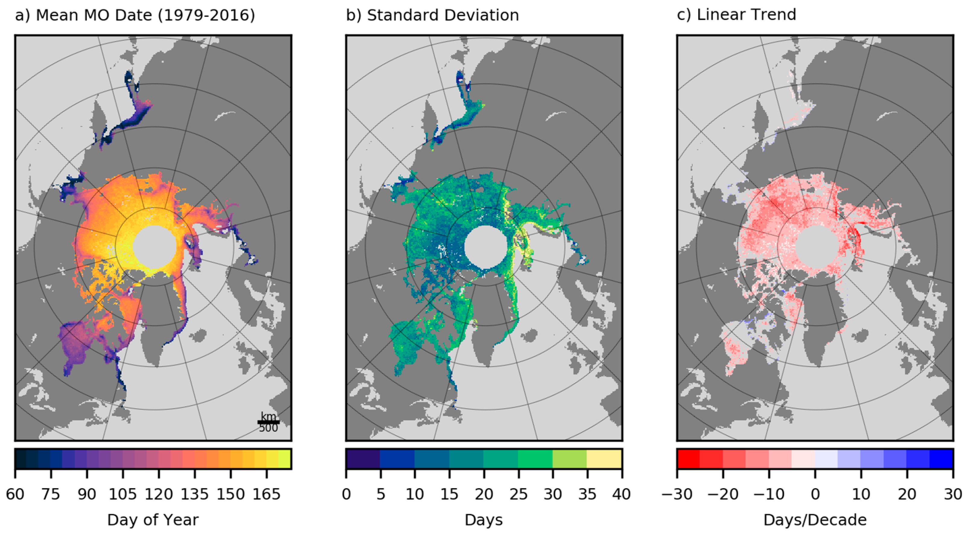
3.1.1. Spatial Distribution of Mean and STD of MO
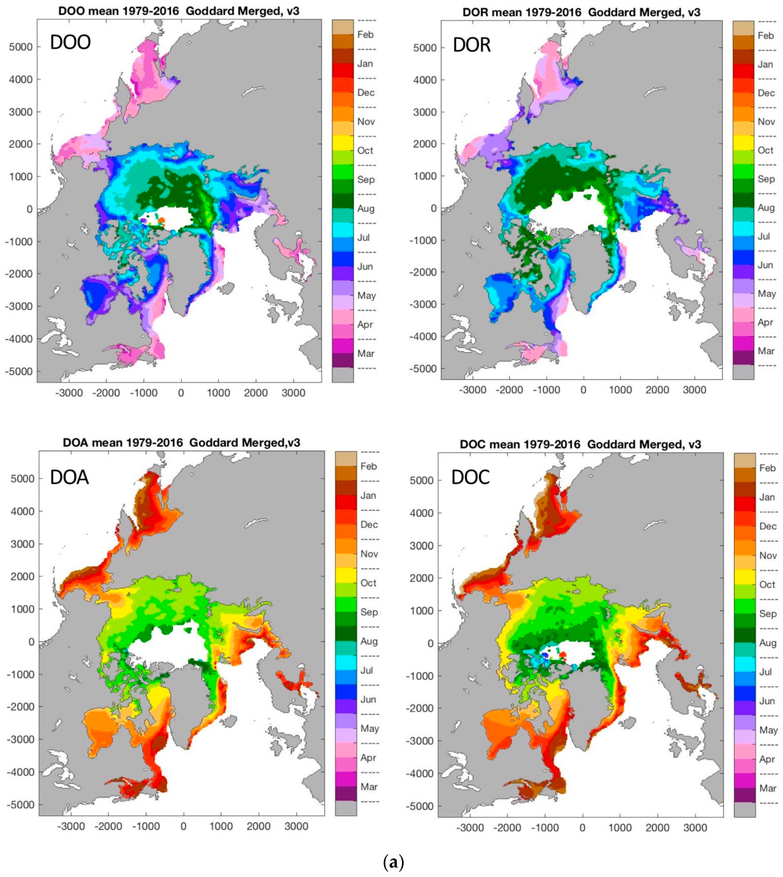
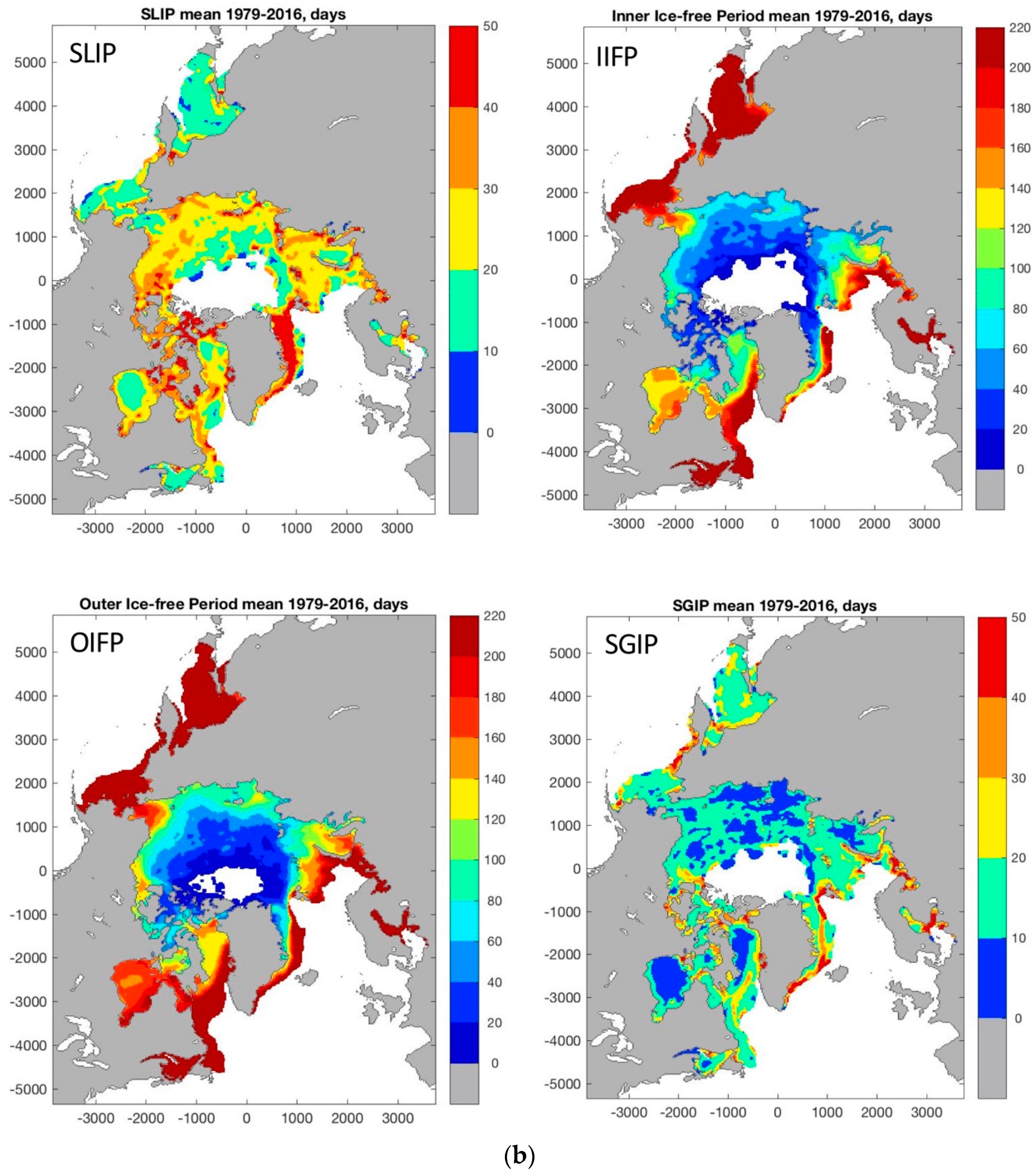
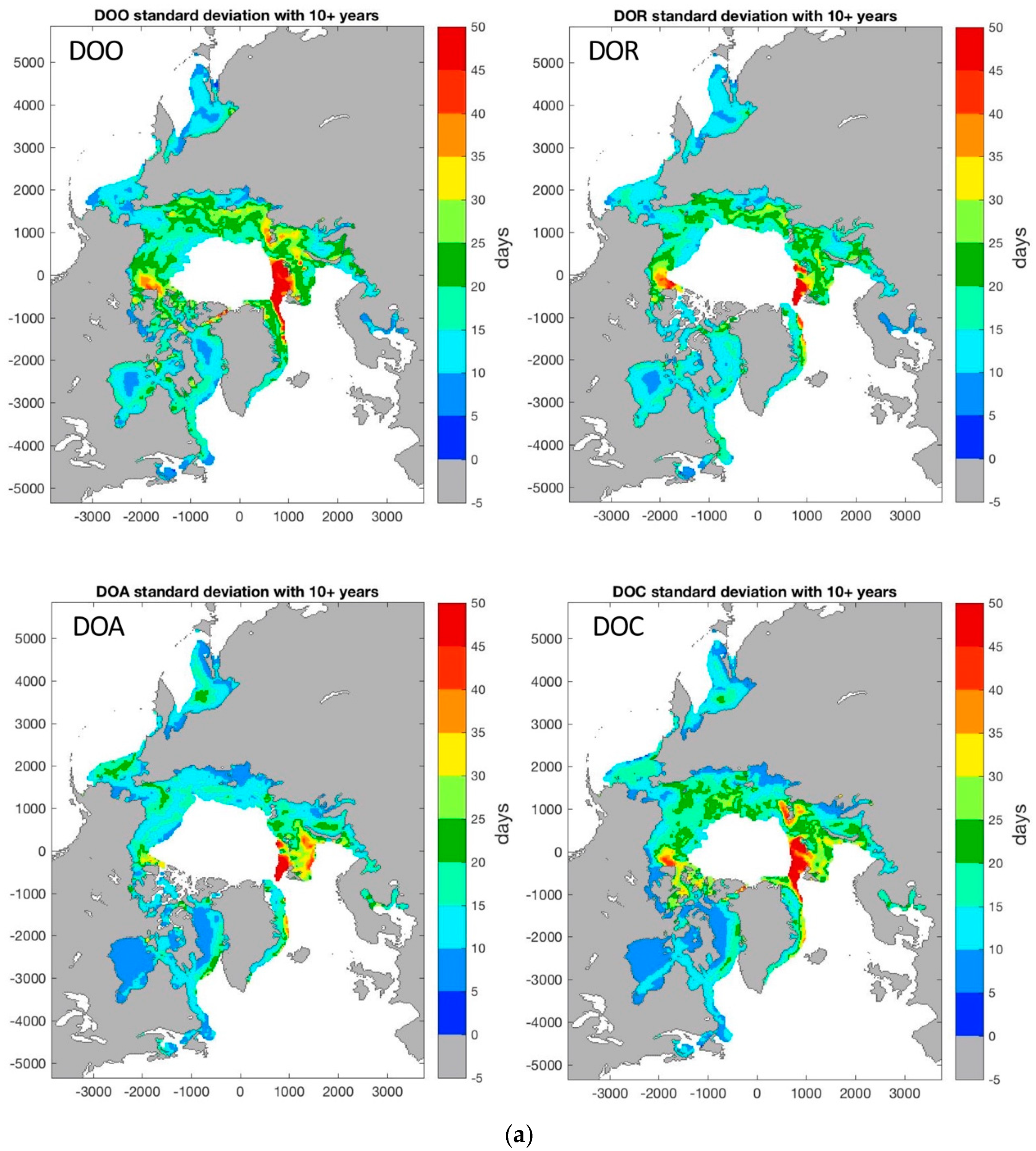
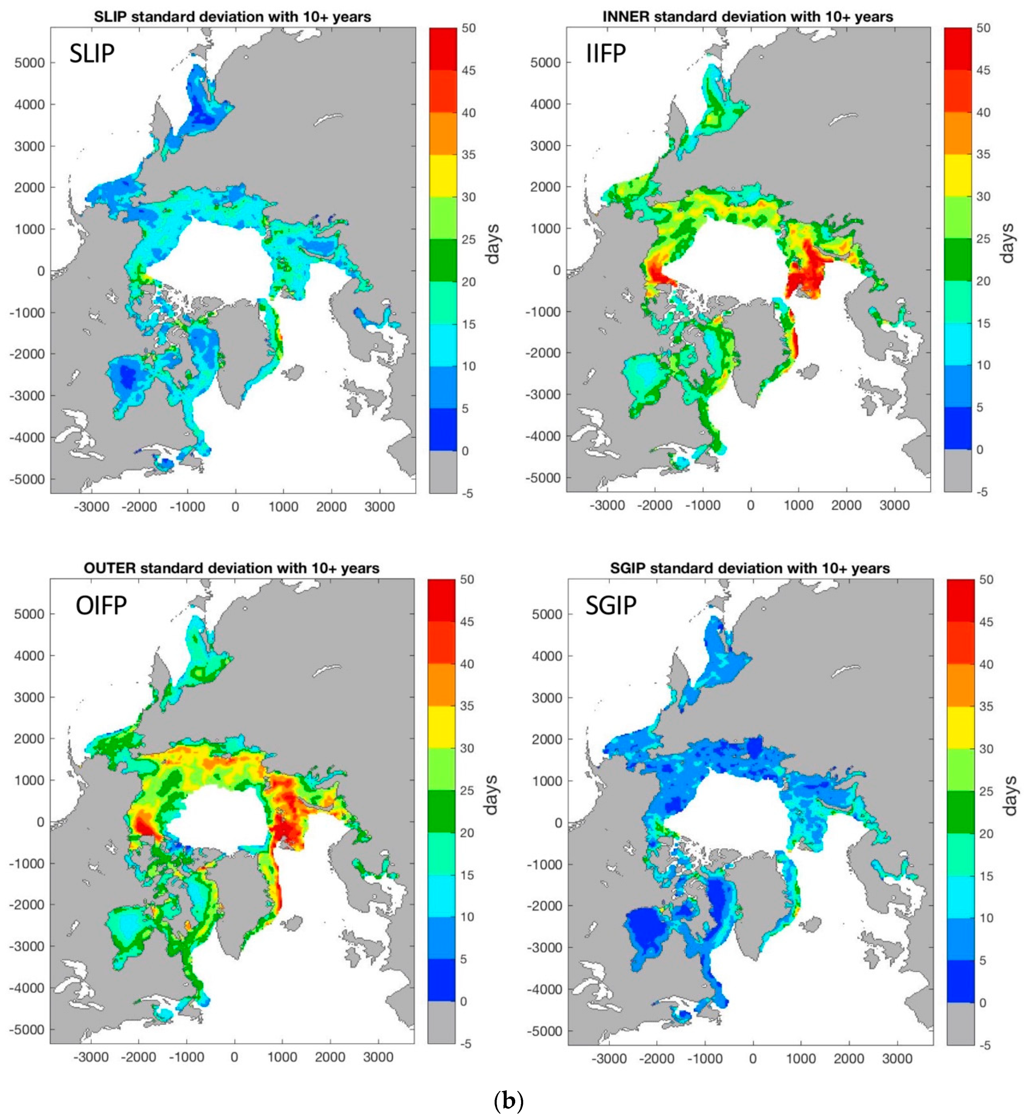
3.1.2. Spatial Distribution of Mean and STD of DOx and Periods
3.2. Decade Trends of Dates and Periods
3.2.1. Spatial Distribution of Decadal Trends of MO
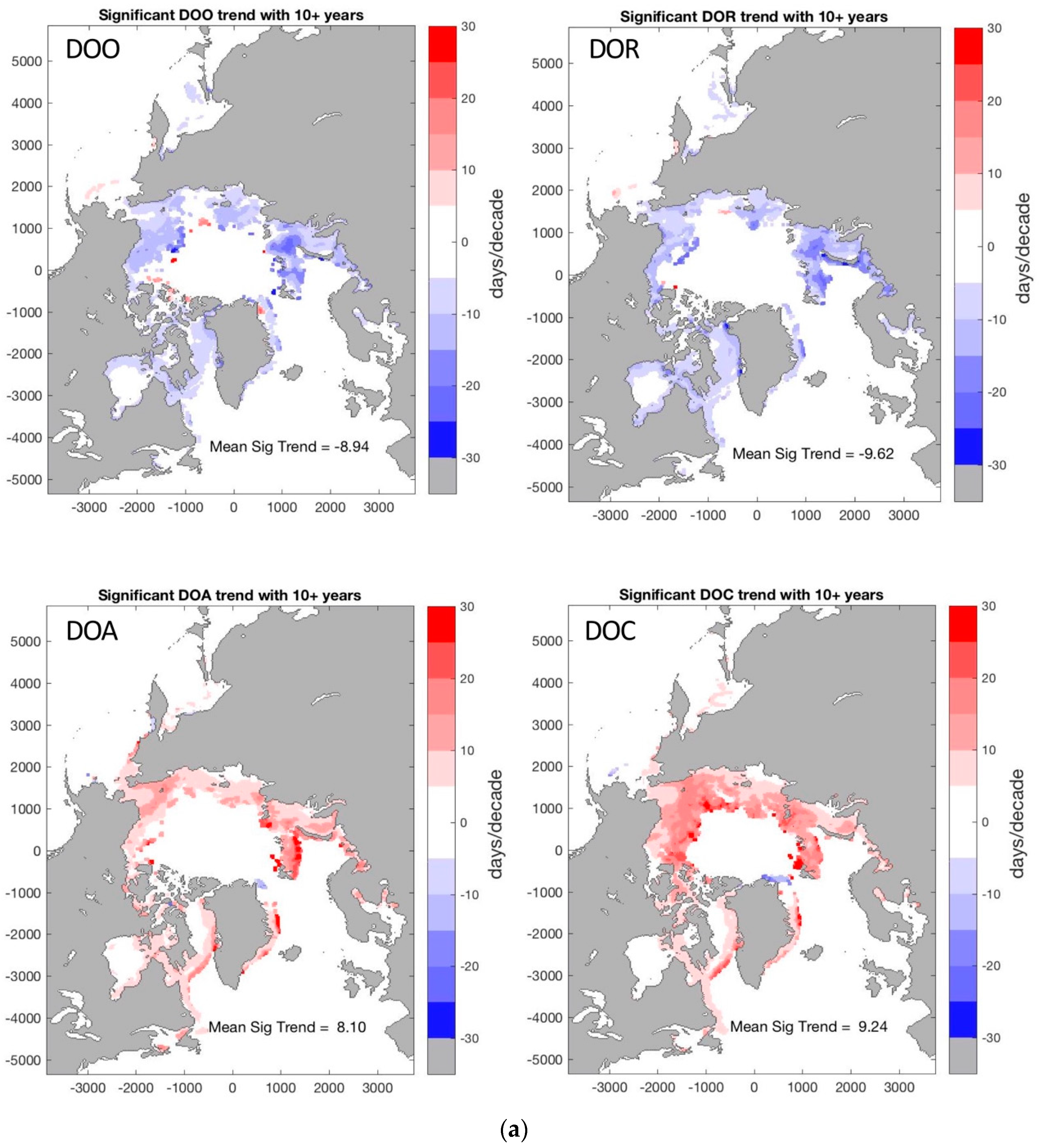
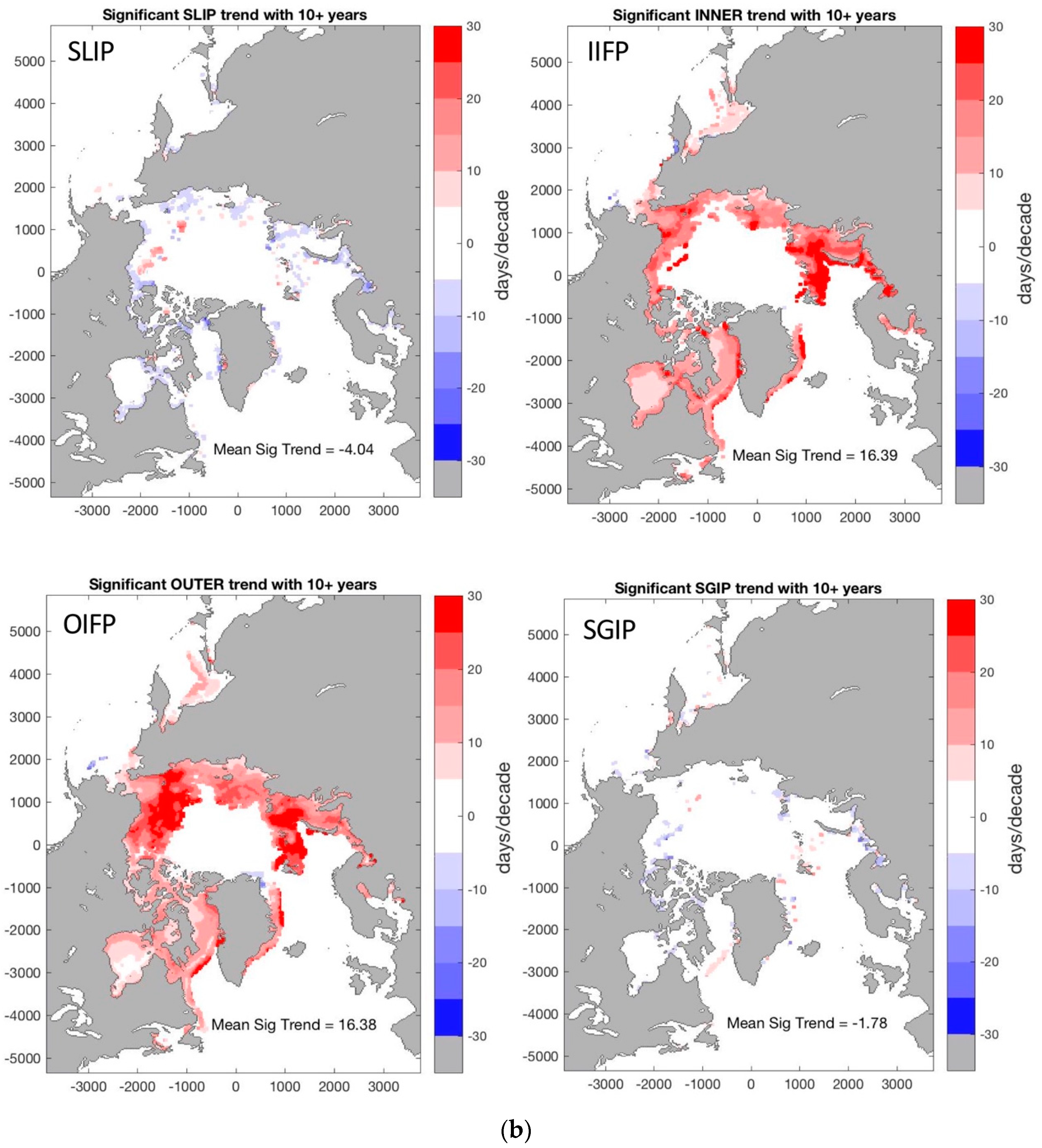
3.2.2. Spatial Distribution of Significant Trends of DOx and Periods
3.2.3. Decadal Trends of Arctic Averaged Dates and Periods
Decadal Arctic MO Trends
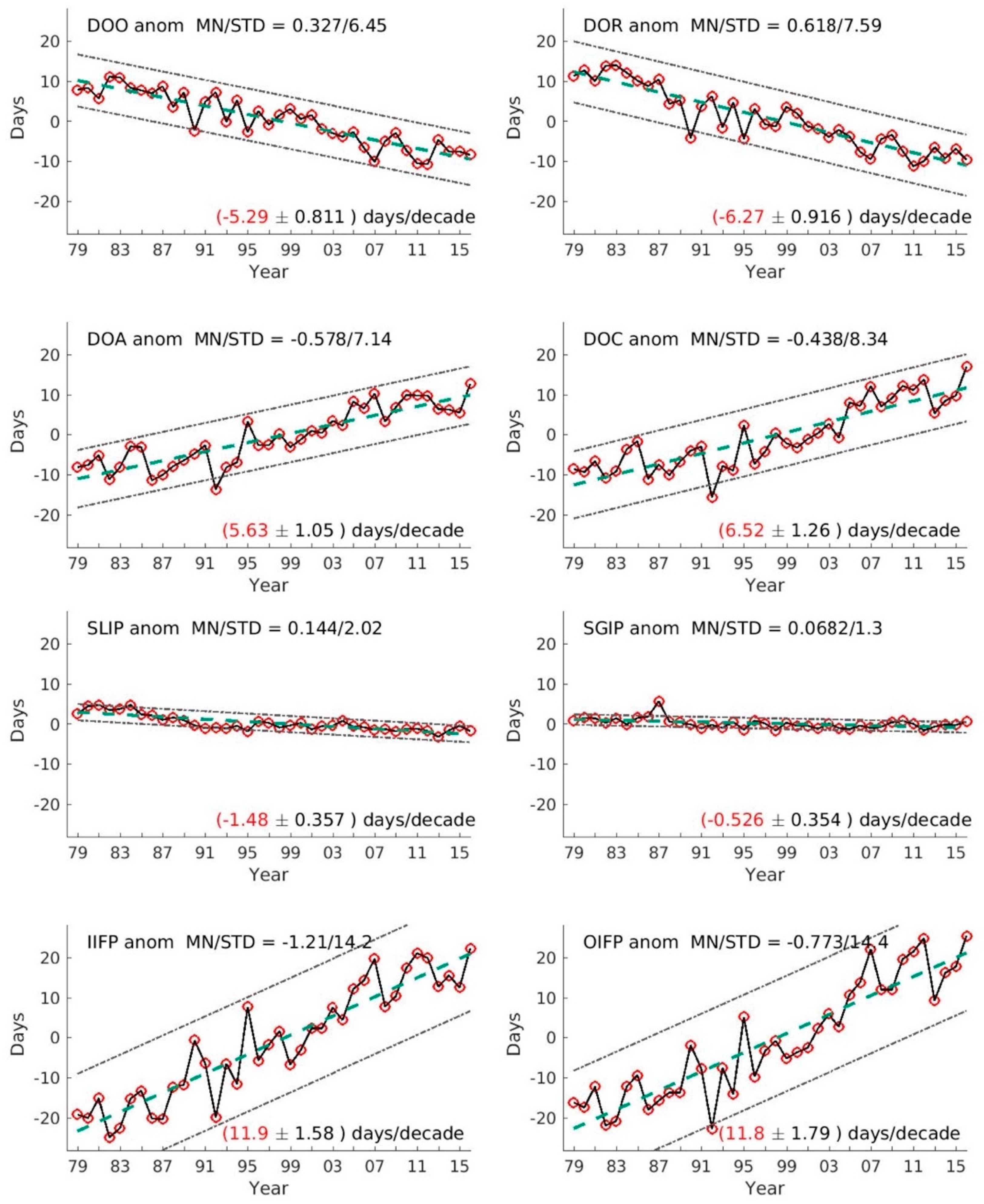
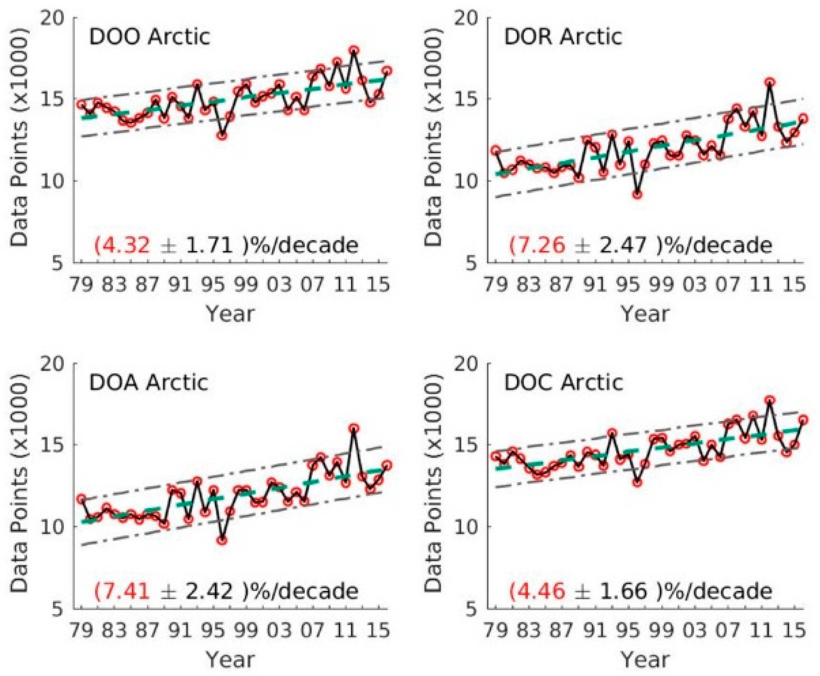
Arctic DOx and Periods Decadal Trends
4. Discussion
5. Conclusions
Author Contributions
Funding
Acknowledgments
Conflicts of Interest
References
- Acacia Communications (ACIA). Impacts of a Warming Arctic—Arctic Climate Impact Assessment; Cambridge University Press: Cambriddge, UK, 2004; p. 140. [Google Scholar]
- Intergovernmental Panel on Climate Change (IPCC). Climate Change 2014: Synthesis Report; Contribution of Working Groups I, II and III to the Fifth Assessment Report of the Intergovernmental Panel on Climate Change; Core Writing Team, Pachauri, R.K., Meyer, L.A., Eds.; IPCC: Geneva, Switzerland, 2014; p. 151. [Google Scholar]
- Stanitski, D.M.; Intrieri, J.M.; Druckenmiller, M.L.; Fetterer, F.; Gerst, M.D.; Kenney, M.A.; Meier, W.N.; Overland, J.; Stroeve, J.; Trainor, S.F. Indicators for a Changing Arctic. Clim. Chang. 2018. under review. [Google Scholar]
- Steele, M.; Dickinson, S.; Zhang, J.; Lindsay, R. Seasonal ice loss in the Beaufort Sea: Toward synchrony and prediction. J. Geophys. Res. Oceans 2015, 120, 1118–1132. [Google Scholar] [CrossRef]
- Steele, M.; Dickinson, S. The phenology of Arctic Ocean surface warming. J. Geophys. Res. 2016, 121, 6847–6861. [Google Scholar] [CrossRef] [PubMed]
- Markus, T.; Stroeve, J.C.; Miller, J. Recent changes in Arctic sea ice melt onset, freezeup, and melt season length. J. Geophys. Res 2009, 114, C12. [Google Scholar] [CrossRef]
- U.S. National Ice Center, Current Daily Ice Analysis. 2018. Available online: https://www.natice.noaa.gov/Main_Products.htm (accessed on 26 July 2018).
- Mortin, J.; Svensson, G.; Graversen, R.G.; Kapsch, M.; Stroeve, J.C.; Boisvert, L.N. Melt onset over Arctic sea ice controlled by atmospheric moisture transport. Geophys. Res. Lett. 2016, 43, 6636–6642. [Google Scholar] [CrossRef]
- Bliss, A.; Miller, J.; Meier, W.N. Comparison of Passive Microwave-Derived Early Melt Onset Records on Arctic Sea Ice. Remote Sens. 2017, 9, 199. [Google Scholar] [CrossRef]
- Liu, Z.; Schweiger, A. Synoptic Conditions, Clouds, and Sea Ice Melt Onset in the Beaufort and Chukchi Seasonal Ice Zone. J. Clim. 2017, 30, 6999–7016. [Google Scholar] [CrossRef]
- Wang, L.; Derksen, C.; Brown, R.; Markus, T. Recent changes in pan-Arctic melt onset from satellite passive microwave measurements. Geophys. Res. Lett. 2013, 40, 522–528. [Google Scholar] [CrossRef]
- Stammerjohn, S.; Massom, R.; Rind, D.; Martinson, D. Regions of rapid sea ice change: An inter-hemispheric seasonal comparison. Geophys. Res. Lett. 2012, 39, L06501. [Google Scholar] [CrossRef]
- Parkinson, C.L. Spatial Patterns of Increases and Decreases in the Length of the Sea Ice Season in the North Polar Region, 1979–1986. J. Geophys. Res 1992, 97, 14377–14388. [Google Scholar] [CrossRef]
- Parkinson, C.L. Spatially mapped reductions in the length of the Arctic sea ice season. Geophys. Res. Lett. 2014, 41, 4316–4322. [Google Scholar] [CrossRef] [PubMed]
- Stroeve, J.C.; Crawford, A.D.; Stammerjohn, S. Using timing of ice retreat to predict timing of fall freeze-up in the Arctic. Geophys. Res. Lett. 2016, 43, 6332–6340. [Google Scholar] [CrossRef]
- Perovich, D.K.; Nghiem, S.V.; Markus, T.; Schweiger, A. Seasonal evolution and interannual variability of the local solar energy absorbed by the Arctic sea ice-ocean system. J. Geophys. Res 2007, 112, C3. [Google Scholar] [CrossRef]
- Kapsch, M.L.; Graversen, R.G.; Economou, T.; Tjernström, M. The importance of spring atmospheric conditions for predictions of the Arctic summer sea ice extent. Geophys. Res. Lett. 2014, 41, 5288–5296. [Google Scholar] [CrossRef]
- Cavalieri, D.J. A microwave technique for mapping thin sea ice. J. Geophys. Res 1994, 99, 12561–12572. [Google Scholar] [CrossRef]
- Comiso, J.C.; Meier, W.N.; Gersten, R. Variability and trends in the Arctic Sea ice cover: Results from different techniques. J. Geophys. Res. Ocean. 2017, 122, 6883–6900. [Google Scholar] [CrossRef]
- Meier, W.N.; Fetterer, F.; Savoie, M.; Mallory, S.; Duerr, R.; Stroeve, J. NOAA/NSIDC Climate Data Record of Passive Microwave Sea Ice Concentration, Version 3; National Snow and Ice Data Center (NSIDC): Boulder, CO, USA, 2017. [Google Scholar]
- Peng, G.; Meier, M.N.; Scott, D.J.; Savoie, M. A long-term and reproducible passive microwave sea ice concentration data record for climate studies and monitoring. Earth-Syst. Sci. Data 2013, 5, 311–318. [Google Scholar] [CrossRef]
- Drobot, S.D.; Anderson, M.R. An improved method for determining snowmelt onset dates over Arctic sea ice using scanning multichannel microwave radiometer and Special Sensor Microwave/Imager data. J. Geophys. Res. Atmos. 2001, 106, 24033–24049. [Google Scholar] [CrossRef]
- Anderson, M.R.; Bliss, A.C.; Drobot, S.D. Snow Melt Onset Over Arctic Sea Ice from SMMR and SSM/I-SSMIS Brightness Temperatures, Version 3; National Snow and Ice Data Center (NSIDC): Boulder, CO, USA, 2014. [Google Scholar]
- Stroeve, J.C.; Markus, T.; Boisvert, L.; Miller, J.; Barrett, A. Changes in Arctic melt season and implications for sea ice loss. Geophys. Res. Lett. 2014, 41, 1216–1225. [Google Scholar] [CrossRef]
- Mahmud, M.S.; Howell, S.E.L.; Geldsetzer, T.; Yackel, J. Detection of melt onset over the northern Canadian Arctic Archipelago sea ice from RADARSAT, 1997–2014. Remote Sens. Environ. 2016, 178, 59–69. [Google Scholar] [CrossRef]
- Hochheim, K.P.; Barber, D.G. An Update on the Ice Climatology of the Hudson Bay System. Arct. Antarct. Alp. Res. 2014, 46, 66–83. [Google Scholar] [CrossRef]
- Onarheim, I.H.; Smedsrud, L.H.; Ingvaldsen, R.B.; Nilsen, F. Loss of sea ice during winter north of Svalbard. Tellus A Dyn. Meteorol. Oceanogr. 2014, 66. [Google Scholar] [CrossRef]
- Serreze, M.C.; Crawford, A.D.; Stroeve, J.C.; Barrett, A.P.; Woodgate, R.A. Variability, trends, and predictability of seasonal sea ice retreat and advance in the Chukchi Sea. J. Geophys. Res. Ocean. 2016, 121, 7308–7325. [Google Scholar] [CrossRef]
- Steele, M.; Zhang, J.; Ermold, W. Mechanisms of summertime upper Arctic Ocean warming and the effect on sea ice melt. J. Geophys. Res. 2010, 115, C11004. [Google Scholar] [CrossRef]
- Smith, M.; Stammerjohn, S.; Persson, O.; Rainville, L.; Liu, G.; Perrie, W.; Robertson, R.; Jackson, J.; Thomson, J.; Smith, M. Episodic reversal of autumn ice advance caused by release of ocean heat in the Beaufort Sea. J. Geophys. Res. Ocean. 2018, 123, 3164–3185. [Google Scholar] [CrossRef]
- Cavalieri, D.J.; Parkinson, C.L. Arctic sea ice variability and trends, 1979–2010. Cryosphere 2012, 6, 881–889. [Google Scholar] [CrossRef]
- Frey, K.E.; Moore, G.W.K.; Cooper, L.W.; Grebmeier, J.M. Divergent patterns of recent sea ice cover across the Bering, Chukchi, and Beaufort seas of the Pacific Arctic Region. Prog. Oceanogr. 2015, 136, 32–49. [Google Scholar] [CrossRef]
- Cavalieri, D.J.; Parkinson, C.L.; Gloersen, P.; Comiso, J.C.; Zwally, H.J. Deriving long-term time series of sea ice cover from satellite passive-microwave multisensor data sets. J. Geophys. Res. 1999, 104, 15803–15814. [Google Scholar] [CrossRef]
- Bliss, A.C.; Anderson, M.R. Arctic sea ice melt onset from passive microwave satellite data: 1979–2012. Cryosphere Discuss. 2014, 8. [Google Scholar] [CrossRef]
- Peng, G.; Meier, W.N. Temporal and regional variability of Arctic sea-ice coverage from satellite data. Ann. Glaciol. 2017, 191–200. [Google Scholar] [CrossRef]
- Bliss, A.C.; Anderson, M.R. Daily Area of Snow Melt Onset on Arctic Sea Ice from Passive Microwave Satellite Observations 1979–2012. Remote Sens. 2014, 6, 11283–11314. [Google Scholar] [CrossRef]
- Bliss, A.C.; Steele, M.; Peng, G.; Meier, W.N.; Dickinson, S. Regional Variability of Arctic Sea Ice Melt Season Indicators from a Passive Microwave Climate Data Record. Environ. Res. Lett. 2018. under review. [Google Scholar]
- Andersen, S.; Tonboe, R.; Kern, S.; Schyberg, H. Improved retrieval of sea ice total concentration from spaceborne passive microwave observations using numerical weather prediction model fields: An intercomparison of nine algorithms. Remote Sens. Environ. 2006, 104, 374–392. [Google Scholar] [CrossRef]
- Ivanova, N.; Pedersen, L.T.; Tonboe, R.T.; Kern, S.; Heygster, G.; Lavergne, T.; Sørensen, A.; Saldo, R.; Dybkjær, G.; Brucker, L.; et al. Inter-comparison and evaluation of sea ice algorithms: Towards further identification of challenges and optimal approach using passive microwave observations. Cryosphere 2015, 9, 1797–1817. [Google Scholar] [CrossRef]


| Acronym | Definition and Description |
|---|---|
| MO | Day of snow and ice melting onset |
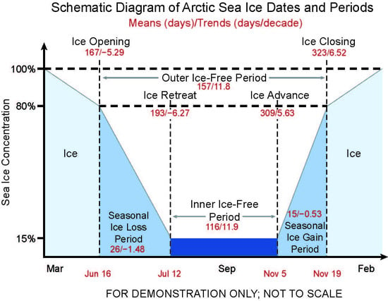
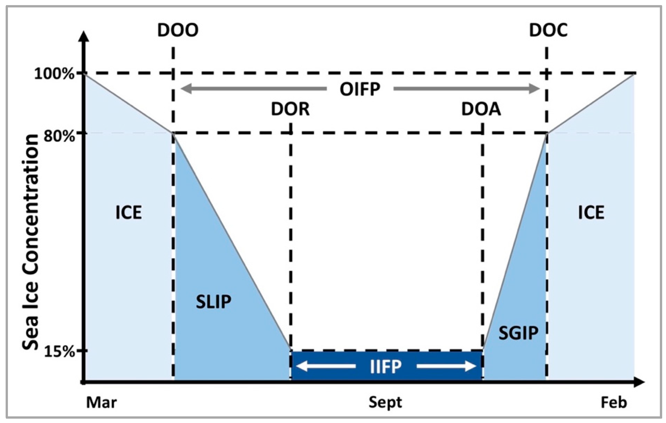
| DOO | Day of opening, last day sea ice concentration (SIC) drops below 80% before the first summer minimum |
| DOR | Day of retreat, last day SIC drops below 15% before the first summer minimum |
| DOA | First day of advance, first day SIC increases above 15% after the last summer minimum |
| DOC | First day of closing, first day SIC increases above 80% after the last summer minimum |
| SLIP | Seasonal loss of ice period, defined as DOR–DOO |
| SGIP | Seasonal gain of ice period, defined as DOC–DOA |
| IIFP | Inner ice-free period (open ocean), defined as DOA–DOR |
| OIFP | Outer ice-free period, defined as DOC–DOO |
| Case Type | Mean | Min | Max | STD | Trend (cell/decade) | ME (cell/decade) |
|---|---|---|---|---|---|---|
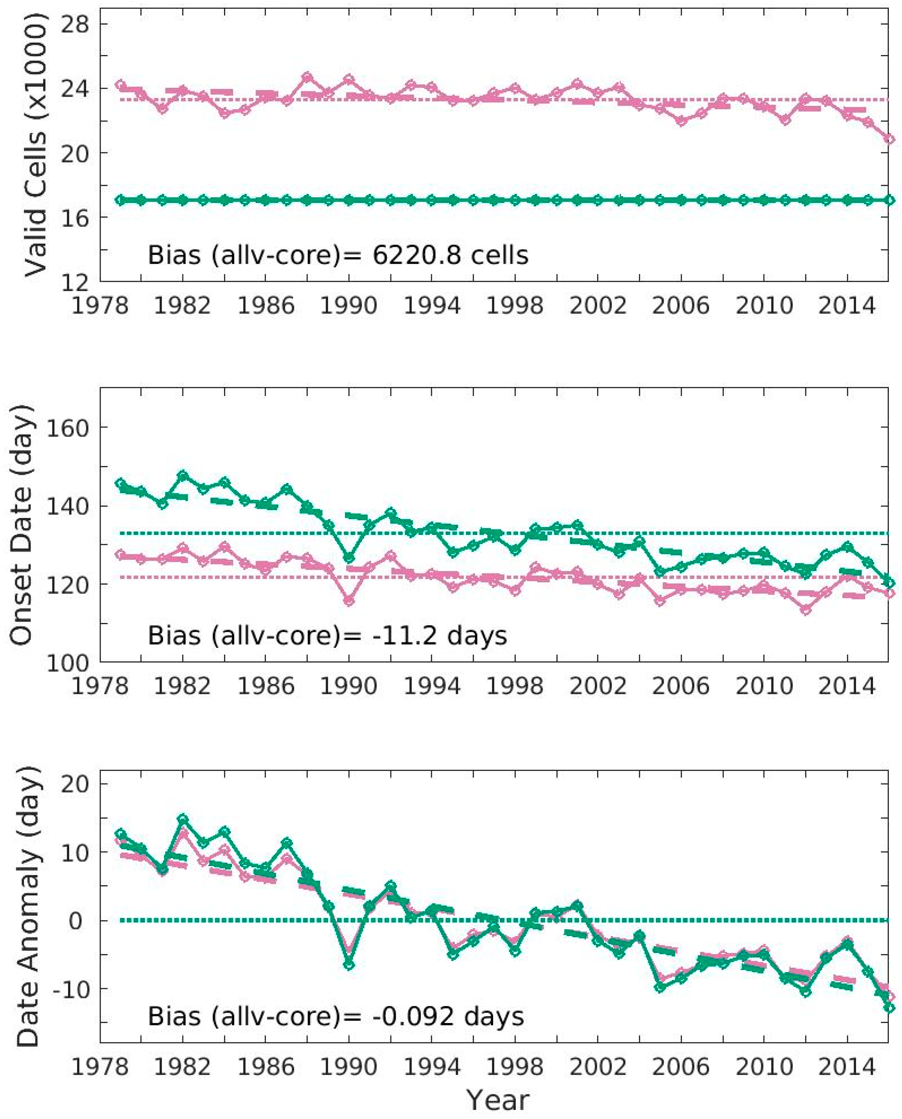
| allv | 23,279 | 20,883 | 24,717 | 802 | −357 | 121 |
| core | 17,058 | 17,058 | 17,058 | 0 | 0 | 0 |
| North Pole Hole Mask | North Pole Hole Area (106 km2) | North Pole Hole Radium (km) | Latitude (°N) | Total Number of Grid Cells | Record Period Used |
|---|---|---|---|---|---|
| SSMIS | 0.029 | 94 | 89.18 | 44 | January 2008–February 2017 |
| SMM/I | 0.31 | 311 | 87.2 | 468 | August 1987–December 2007 |
| SMMR | 1.19 | 611 | 84.5 | 1799 | March 1979–July 1987 |
| Case Type | Mean (day) | Min (day) | Max (day) | STD (day) | Trend (day/decade) | ME (day/decade) | |
|---|---|---|---|---|---|---|---|
| Method I | allv | 121.78 | 113.51 | 129.61 | 4.07 | −2.85 * | 0.96 |
| core | 133.00 | 120.22 | 147.79 | 7.49 | −5.93 * | 2.00 | |
| Method II | allv | −0.092 | −11.15 | 12.89 | 6.49 | −5.23 * | 1.77 |
| core | 0.00 | −12.78 | 14.79 | 7.49 | −5.93 * | 2.00 |
| Case Allv | Case Core | Case Mask a | Case comm b | |||||
|---|---|---|---|---|---|---|---|---|
| Date or Period Type | Mean (day) | # of Records | Mean (day) | # of Records | Mean (day) | # of Records | Mean (day) | # of Records |
| DOO | 176.3 | 570,918 | 174.4 | 249,090 | 165.5 | 456,522 | 166.6 | 446,145 |
| DOR | 191.5 | 456,522 | 188.7 | 150,708 | 191.5 | 456,522 | 192.7 | 446,145 |
| DOA | 309.8 | 452,761 | 315.9 | 150,708 | 309.8 | 452,761 | 308.5 | 446,145 |
| DOC | 309.3 | 560,490 | 312.3 | 246,392 | 323.1 | 446,145 | 323.1 | 446,145 |
| SLIP | 26.0 | 456,522 | 23.53 | 148,010 | 26.0 | 456,522 | 26.1 | 446,145 |
| SGIP | 14.6 | 446,145 | 11.42 | 150,637 | 14.6 | 446,145 | 14.6 | 446,145 |
| IIFP | 117.8 | 452,761 | 127.3 | 150,637 | 117.8 | 452,761 | 115.8 | 446,145 |
| OIFP | 131.9 | 560,490 | 137.9 | 246,392 | 156.5 | 446,145 | 156.5 | 446,145 |
| Date or Period Type | Mean (day) | STD (day) | Trend (day/decade) | ME (day/decade) |
|---|---|---|---|---|
| DOO | 0.33 | 6.45 | −5.29 * | 0.81 |
| DOR | 0.62 | 7.59 | −6.27 * | 0.92 |
| DOA | −0.58 | 7.14 | 5.63 * | 1.05 |
| DOC | −0.44 | 8.34 | 6.52 * | 1.26 |
| SLIP | 0.14 | 2.02 | −1.48 * | 0.36 |
| SGIP | 0.068 | 1.30 | −0.53 * | 0.35 |
| IIFP | −1.21 | 14.2 | 11.9 * | 1.58 |
| OIFP | −0.77 | 14.4 | 11.8 * | 1.79 |
© 2018 by the authors. Licensee MDPI, Basel, Switzerland. This article is an open access article distributed under the terms and conditions of the Creative Commons Attribution (CC BY) license (http://creativecommons.org/licenses/by/4.0/).
Share and Cite
Peng, G.; Steele, M.; Bliss, A.C.; Meier, W.N.; Dickinson, S. Temporal Means and Variability of Arctic Sea Ice Melt and Freeze Season Climate Indicators Using a Satellite Climate Data Record. Remote Sens. 2018, 10, 1328. https://doi.org/10.3390/rs10091328
Peng G, Steele M, Bliss AC, Meier WN, Dickinson S. Temporal Means and Variability of Arctic Sea Ice Melt and Freeze Season Climate Indicators Using a Satellite Climate Data Record. Remote Sensing. 2018; 10(9):1328. https://doi.org/10.3390/rs10091328
Chicago/Turabian StylePeng, Ge, Michael Steele, Angela C. Bliss, Walter N. Meier, and Suzanne Dickinson. 2018. "Temporal Means and Variability of Arctic Sea Ice Melt and Freeze Season Climate Indicators Using a Satellite Climate Data Record" Remote Sensing 10, no. 9: 1328. https://doi.org/10.3390/rs10091328
APA StylePeng, G., Steele, M., Bliss, A. C., Meier, W. N., & Dickinson, S. (2018). Temporal Means and Variability of Arctic Sea Ice Melt and Freeze Season Climate Indicators Using a Satellite Climate Data Record. Remote Sensing, 10(9), 1328. https://doi.org/10.3390/rs10091328