UAV Multispectral Imagery Can Complement Satellite Data for Monitoring Forest Health

Abstract
1. Introduction
2. Methods
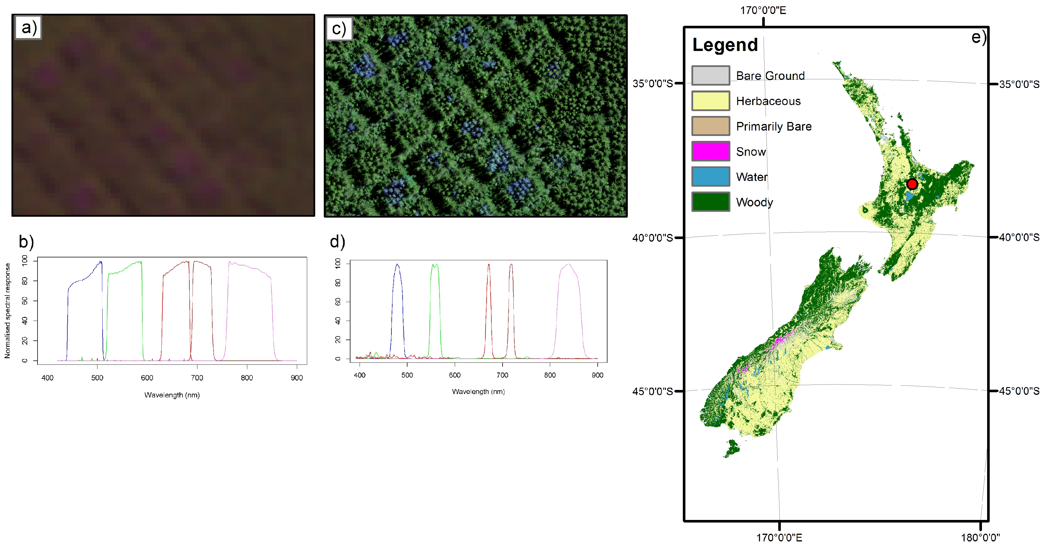
2.1. Study Site
2.2. Experimental Design
2.3. UAV Imagery
2.4. Satellite Imagery
2.5. Image Processing
2.6. Tree Health Data
2.7. Statistical Analysis
3. Results
3.1. Data Summary
3.2. Spectral Indices
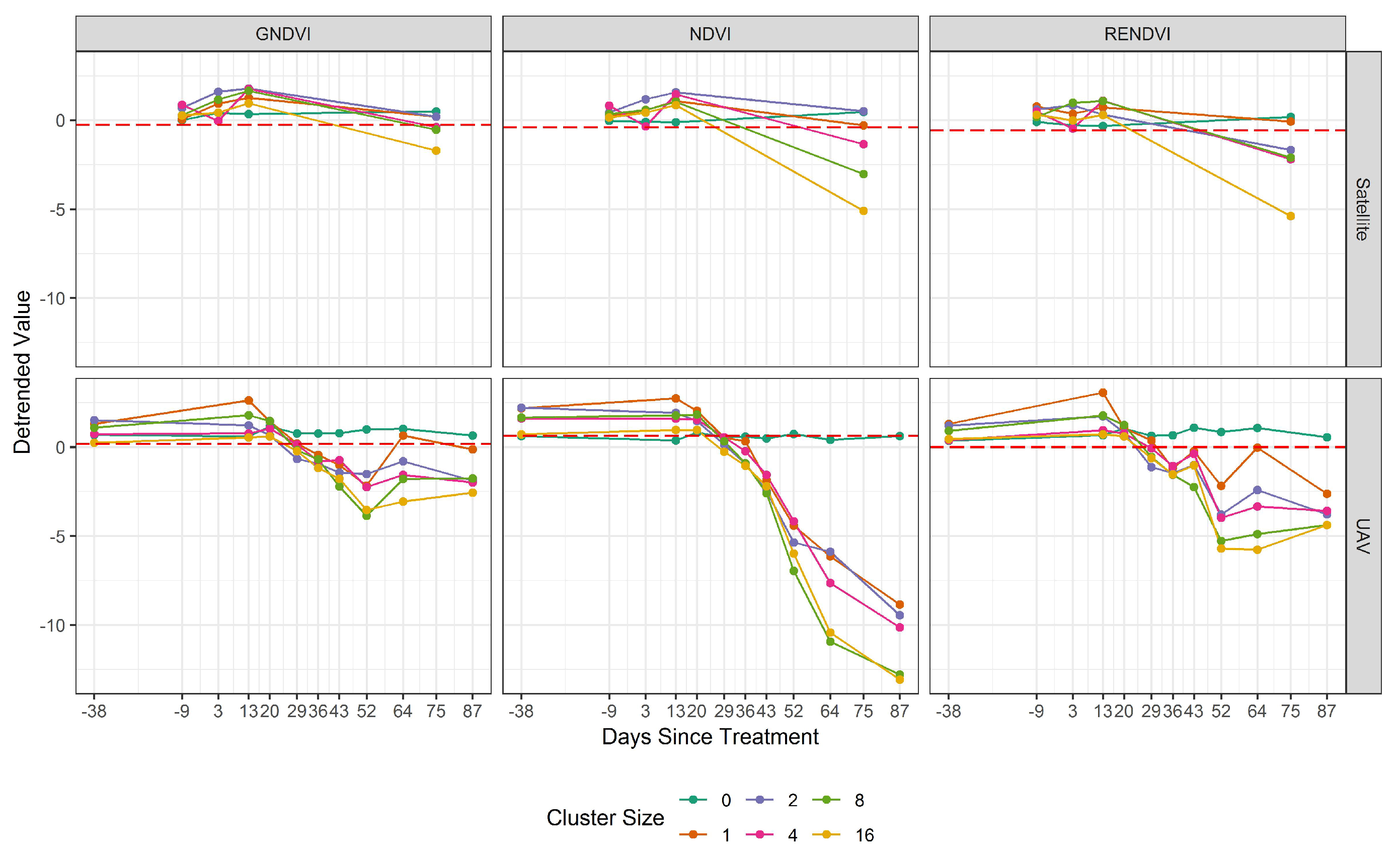
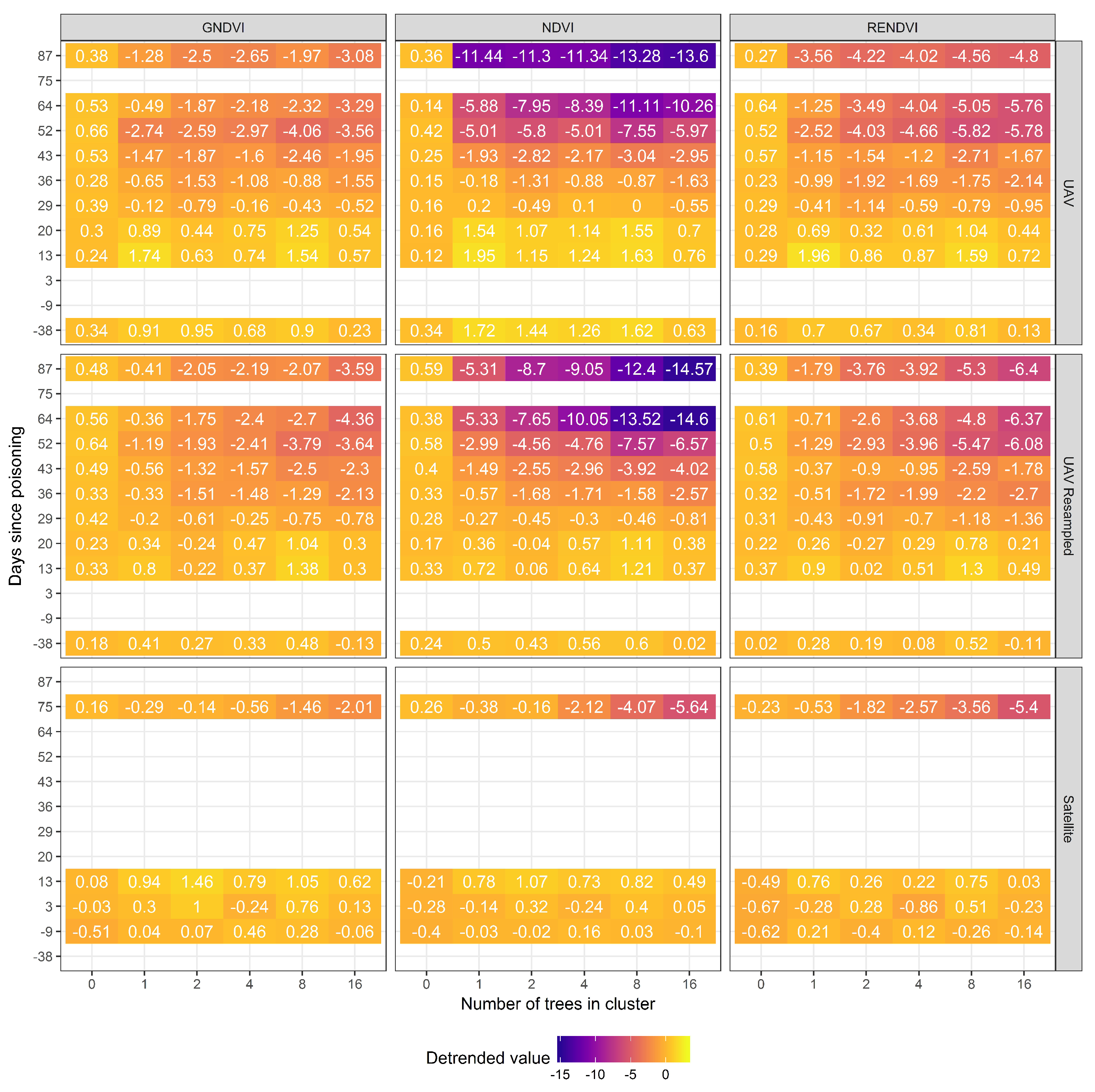
3.3. Spatial Resolution
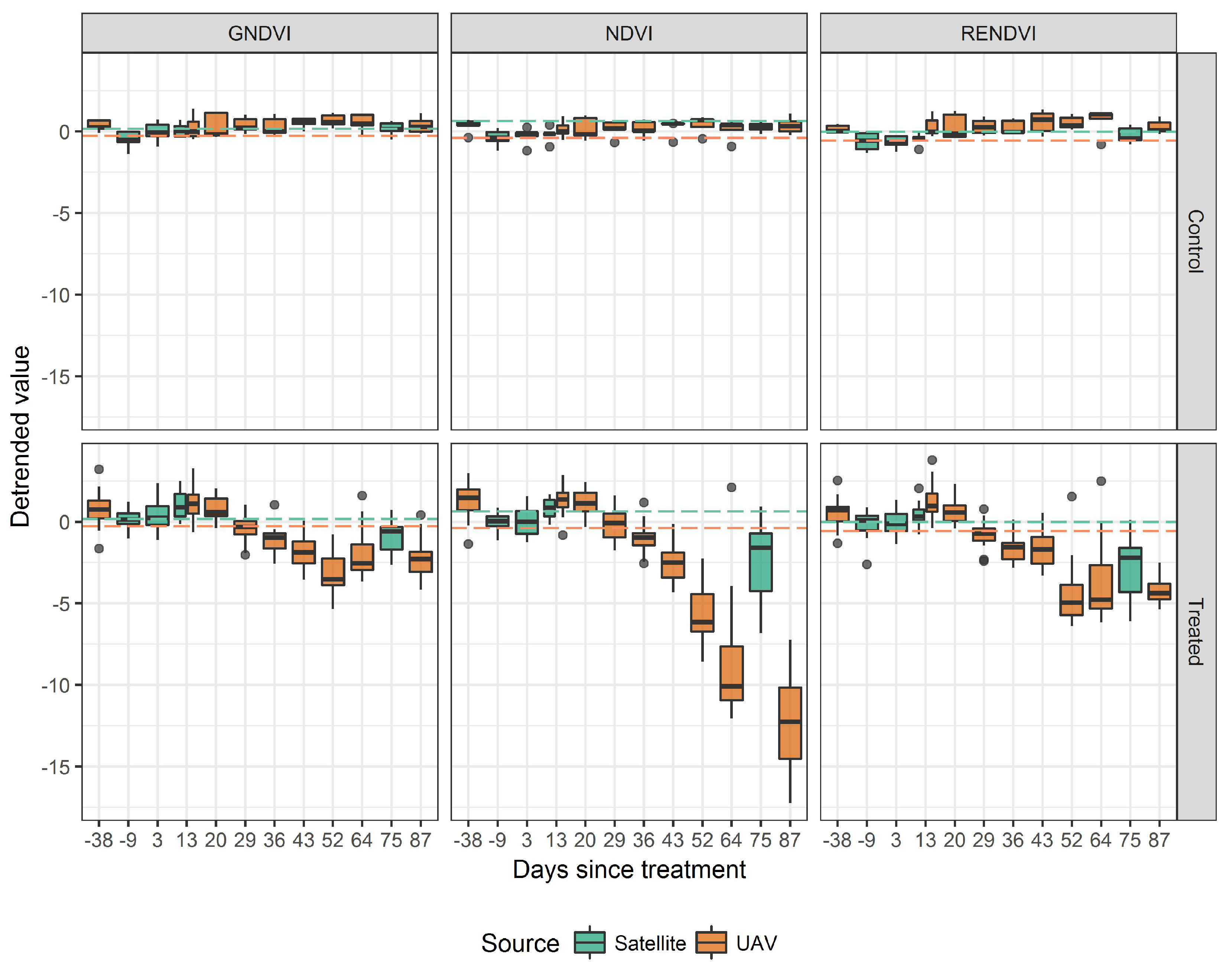
3.4. Comparing UAV and Satellite Imagery
4. Discussion
5. Conclusions
Author Contributions
Funding
Acknowledgments
Conflicts of Interest
References
- Moore, J.R.; Dash, J.P.; Lee, J.R.; McKinley, R.B.; Dungey, H.S. Quantifying the influence of seedlot and stand density on growth, wood properties and the economics of growing radiata pine. Forestry 2017, 91, 327–340. [Google Scholar] [CrossRef]
- Watt, M.S.; Kimberley, M.O.; Dash, J.P.; Harrison, D. Spatial prediction of optimal final stand density for even-aged plantation forests using productivity indices. Can. J. For. Res. 2017, 47, 527–535. [Google Scholar] [CrossRef]
- Klapste, J.; Suontama, M.; Telfer, E.; Graham, N.; Low, C.; Stovold, T.; McKinley, R.; Dungey, H. Exploration of genetic architecture through sib-ship reconstruction in advanced breeding population of Eucalyptus nitens. PLoS ONE 2017, 12, e0185137. [Google Scholar] [CrossRef] [PubMed]
- Li, Y.; Xue, J.; Clinton, P.W.; Dungey, H.S. Genetic parameters and clone by environment interactions for growth and foliar nutrient concentrations in radiata pine on 14 widely diverse New Zealand sites. Tree Genet. Genomes 2015, 11, 10. [Google Scholar] [CrossRef]
- Maggard, A.O.; Will, R.E.; Wilson, D.S.; Meek, C.R.; Vogel, J.G. Fertilization can compensate for decreased water availability by increasing the efficiency of stem volume production per unit of leaf area for loblolly pine (Pinus taeda) stands. Can. J. For. Res. 2017, 47, 445–457. [Google Scholar] [CrossRef]
- Watt, M.S.; Dash, J.P.; Bhandari, S.; Watt, P. Comparing parametric and non-parametric methods of predicting Site Index for radiata pine using combinations of data derived from environmental surfaces, satellite imagery and airborne laser scanning. For. Ecol. Manag. 2015, 357, 1–9. [Google Scholar] [CrossRef]
- Watt, M.S.; Dash, J.P.; Watt, P.; Bhandari, S. Multi-sensor modelling of a forest productivity index for radiata pine plantations. N. Z. J. For. Sci. 2016, 46, 9. [Google Scholar] [CrossRef]
- Pearse, G.D.; Morgenroth, J.; Watt, M.S.; Dash, J.P. Optimising prediction of forest leaf area index from discrete airborne lidar. Remote Sens. Environ. 2017, 200, 220–239. [Google Scholar] [CrossRef]
- Paoletti, E. Impact of ozone on Mediterranean forests: A review. Environ. Pollut. 2006, 144, 463–474. [Google Scholar] [CrossRef] [PubMed]
- Marco, A.D.; Vitale, M.; Popa, I.; Anav, A.; Badea, O.; Silaghi, D.; Leca, S.; Screpanti, A.; Paoletti, E. Ozone exposure affects tree defoliation in a continental climate. Sci. Total Environ. 2017, 596–597, 396–404. [Google Scholar] [CrossRef] [PubMed]
- Moore, J.R.; Watt, M.S. Modelling the influence of predicted future climate change on the risk of wind damage within New Zealand’s planted forests. Glob. Chang. Biol. 2015, 21, 3021–3035. [Google Scholar] [CrossRef] [PubMed]
- Dash, J.P.; Watt, M.S.; Pearse, G.D.; Heaphy, M.; Dungey, H.S. Assessing very high resolution UAV imagery for monitoring forest health during a simulated disease outbreak. ISPRS J. Photogramm. Remote Sens. 2017, 131, 1–14. [Google Scholar] [CrossRef]
- Bulman, L.S.; Bradshaw, R.E.; Fraser, S.; Martín-García, J.; Barnes, I.; Musolin, D.L.; La Porta, N.; Woods, A.J.; Diez, J.J.; Koltay, A.; et al. A worldwide perspective on the management and control of Dothistroma needle blight. For. Pathol. 2016, 46, 472–488. [Google Scholar] [CrossRef]
- Coops, N.; Stanford, M.; Old, K.; Dudzinski, M.; Culvenor, D.; Stone, C. Assessment of Dothistroma Needle Blight of Pinus radiata Using Airborne Hyperspectral Imagery. Phytopathology 2003, 93, 1524–1532. [Google Scholar] [CrossRef] [PubMed]
- Meigs, G.W.; Kennedy, R.E.; Cohen, W.B. A Landsat time series approach to characterize bark beetle and defoliator impacts on tree mortality and surface fuels in conifer forests. Remote Sens. Environ. 2011, 115, 3707–3718. [Google Scholar] [CrossRef]
- Eklundh, L.; Johansson, T.; Solberg, S. Mapping insect defoliation in Scots pine with MODIS time-series data. Remote Sens. Environ. 2009, 113, 1566–1573. [Google Scholar] [CrossRef]
- Fraser, R.; Latifovic, R. Mapping insect-induced tree defoliation and mortality using coarse spatial resolution satellite imagery. Int. J. Remote Sens. 2005, 26, 193–200. [Google Scholar] [CrossRef]
- Pasquarella, V.J.; Bradley, B.A.; Woodcock, C.E. Near-Real-Time Monitoring of Insect Defoliation Using Landsat Time Series. Forests 2017, 8. [Google Scholar] [CrossRef]
- Stone, C.; Penman, T.; Turner, R. Managing drought-induced mortality in Pinus radiata plantations under climate change conditions: A local approach using digital camera data. For. Ecol. Manag. 2012, 265, 94–101. [Google Scholar] [CrossRef]
- Coops, N.C.; Johnson, M.; Wulder, M.A.; White, J.C. Assessment of QuickBird high spatial resolution imagery to detect red attack damage due to mountain pine beetle infestation. Remote Sens. Environ. 2006, 103, 67–80. [Google Scholar] [CrossRef]
- Hicke, J.A.; Logan, J. Mapping whitebark pine mortality caused by a mountain pine beetle outbreak with high spatial resolution satellite imagery. Int. J. Remote Sens. 2009, 30, 4427–4441. [Google Scholar] [CrossRef]
- Poona, N.K.; Ismail, R. Discriminating the occurrence of pitch canker fungus in Pinus radiata trees using QuickBird imagery and artificial neural networks. South. For. 2013, 75, 29–40. [Google Scholar] [CrossRef]
- Abdel-Rahman, E.M.; Mutanga, O.; Adam, E.; Ismail, R. Detecting Sirex noctilio grey-attacked and lightning-struck pine trees using airborne hyperspectral data, random forest and support vector machines classifiers. ISPRS J. Photogramm. Remote Sens. 2014, 88, 48–59. [Google Scholar] [CrossRef]
- Dash, J.P.; Pont, D.; Brownlie, R.K.; Dunningham, A.; Watt, M.S.; Pearse, G.D. Remote sensing for precision forestry. N. Z. J. For. 2016, 64, 12. [Google Scholar]
- Puliti, S.; Ene, L.T.; Gobakken, T.; Næsset, E. Use of partial-coverage UAV data in sampling for large scale forest inventories. Remote Sens. Environ. 2017, 194, 115–126. [Google Scholar] [CrossRef]
- Miller, E.; Dandois, J.P.; Detto, M.; Hall, J.S. Drones as a Tool for Monoculture Plantation Assessment in the Steepland Tropics. Forests 2017, 8. [Google Scholar] [CrossRef]
- Goodbody, T.R.; Coops, N.C.; Marshall, P.L.; Tompalski, P.; Crawford, P. Unmanned aerial systems for precision forest inventory purposes: A review and case study. For. Chron. 2017, 93, 71–81. [Google Scholar] [CrossRef]
- Kachamba, D.J.; Ørka, H.O.; Gobakken, T.; Eid, T.; Mwase, W. Biomass Estimation Using 3D Data from Unmanned Aerial Vehicle Imagery in a Tropical Woodland. Remote Sens. 2016, 8, 968. [Google Scholar] [CrossRef]
- Wallace, L.; Lucieer, A.; Malenovský, Z.; Turner, D.; Vopěnka, P. Assessment of Forest Structure Using Two UAV Techniques: A Comparison of Airborne Laser Scanning and Structure from Motion (SfM) Point Clouds. Forests 2016, 7. [Google Scholar] [CrossRef]
- Messinger, M.; Asner, G.P.; Silman, M. Rapid Assessments of Amazon Forest Structure and Biomass Using Small Unmanned Aerial Systems. Remote Sens. 2016, 8, 615. [Google Scholar] [CrossRef]
- Goodbody, T.R.H.; Coops, N.C.; Tompalski, P.; Crawford, P.; Day, K.J.K. Updating residual stem volume estimates using ALS- and UAV-acquired stereo-photogrammetric point clouds. Int. J. Remote Sens. 2017, 38, 2938–2953. [Google Scholar] [CrossRef]
- Watt, M.S.; Heaphy, M.; Dunningham, A.; Rolando, C. Use of remotely sensed data to characterize weed competition in forest plantations. Int. J. Remote Sens. 2017, 38, 2448–2463. [Google Scholar] [CrossRef]
- Cardil, A.; Vepakomma, U.; Brotons, L. Assessing Pine Processionary Moth Defoliation Using Unmanned Aerial Systems. Forests 2017, 8. [Google Scholar] [CrossRef]
- Näsi, R.; Honkavaara, E.; Lyytikäinen-Saarenmaa, P.; Blomqvist, M.; Litkey, P.; Hakala, T.; Viljanen, N.; Kantola, T.; Tanhuanpää, T.; Holopainen, M. Using UAV-Based Photogrammetry and Hyperspectral Imaging for Mapping Bark Beetle Damage at Tree-Level. Remote Sens. 2015, 7, 15467–15493. [Google Scholar] [CrossRef]
- Michez, A.; Piégay, H.; Lisein, J.; Claessens, H.; Lejeune, P. Classification of riparian forest species and health condition using multi-temporal and hyperspatial imagery from unmanned aerial system. Environ. Monit. Assess. 2016, 188, 146. [Google Scholar] [CrossRef] [PubMed]
- Cruz, H.; Eckert, M.; Meneses, J.; Martínez, J.F. Efficient Forest Fire Detection Index for Application in Unmanned Aerial Systems (UASs). Sensors 2016, 16, 893. [Google Scholar] [CrossRef] [PubMed]
- Yuan, C.; Liu, Z.; Zhang, Y. Aerial Images-Based Forest Fire Detection for Firefighting Using Optical Remote Sensing Techniques and Unmanned Aerial Vehicles. J. Intell. Robot. Syst. 2017, 88, 635–654. [Google Scholar] [CrossRef]
- Mokroš, M.; Výbošťok, J.; Merganič, J.; Hollaus, M.; Barton, I.; Koreň, M.; Tomaštík, J.; Čerňava, J. Early Stage Forest Windthrow Estimation Based on Unmanned Aircraft System Imagery. Forests 2017, 8. [Google Scholar] [CrossRef]
- Samiappan, S.; Turnage, G.; McCraine, C.; Skidmore, J.; Hathcock, L.; Moorhead, R. Post-Logging Estimation of Loblolly Pine (Pinus taeda) Stump Size, Area and Population Using Imagery from a Small Unmanned Aerial System. Drones 2017, 1. [Google Scholar] [CrossRef]
- Fraser, R.H.; van der Sluijs, J.; Hall, R.J. Calibrating Satellite-Based Indices of Burn Severity from UAV-Derived Metrics of a Burned Boreal Forest in NWT, Canada. Remote Sens. 2017, 9, 279. [Google Scholar] [CrossRef]
- Stark, D.J.; Vaughan, I.P.; Evans, L.J.; Kler, H.; Goossens, B. Combining drones and satellite tracking as an effective tool for informing policy change in riparian habitats: A proboscis monkey case study. Remote Sens. Ecol. Conserv. 2018, 4, 44–52. [Google Scholar] [CrossRef]
- Szantoi, Z.; Smith, S.E.; Strona, G.; Koh, L.P.; Wich, S.A. Mapping orangutan habitat and agricultural areas using Landsat OLI imagery augmented with unmanned aircraft system aerial photography. Int. J. Remote Sens. 2017, 38, 2231–2245. [Google Scholar] [CrossRef]
- Marx, A.; McFarlane, D.; Alzahrani, A. UAV data for multi-temporal Landsat analysis of historic reforestation: A case study in Costa Rica. Int. J. Remote Sens. 2017, 38, 2331–2348. [Google Scholar] [CrossRef]
- Puliti, S.; Saarela, S.; Gobakken, T.; Ståhl, G.; Næsset, E. Combining UAV and Sentinel-2 auxiliary data for forest growing stock volume estimation through hierarchical model-based inference. Remote Sens. Environ. 2018, 204, 485–497. [Google Scholar] [CrossRef]
- Abdollahnejad, A.; Panagiotidis, D.; Surový, P. Estimation and Extrapolation of Tree Parameters Using Spectral Correlation between UAV and Pléiades Data. Forests 2018, 9, 85. [Google Scholar] [CrossRef]
- Rullan-Silva, C.; Olthoff, A.; de la Mata, J.D.; Pajares-Alonso, J. Remote monitoring of forest insect defoliation-A Review. For. Syst. 2013, 22, 377–391. [Google Scholar] [CrossRef]
- Garrity, S.R.; Allen, C.D.; Brumby, S.P.; Gangodagamage, C.; McDowell, N.G.; Cai, D.M. Quantifying tree mortality in a mixed species woodland using multitemporal high spatial resolution satellite imagery. Remote Sens. Environ. 2013, 129, 54–65. [Google Scholar] [CrossRef]
- Meddens, A.J.; Hicke, J.A. Spatial and temporal patterns of Landsat-based detection of tree mortality caused by a mountain pine beetle outbreak in Colorado, USA. For. Ecol. Manag. 2014, 322, 78–88. [Google Scholar] [CrossRef]
- Havašová, M.; Bucha, T.; Ferenčík, J.; Jakuš, R. Applicability of a vegetation indices-based method to map bark beetle outbreaks in the High Tatra Mountains. Ann. For. Res. 2015, 58, 295–310. [Google Scholar] [CrossRef]
- Goodwin, N.R.; Coops, N.C.; Wulder, M.A.; Gillanders, S.; Schroeder, T.A.; Nelson, T. Estimation of insect infestation dynamics using a temporal sequence of Landsat data. Remote Sens. Environ. 2008, 112, 3680–3689. [Google Scholar] [CrossRef]
- Eitel, J.U.; Vierling, L.A.; Litvak, M.E.; Long, D.S.; Schulthess, U.; Ager, A.A.; Krofcheck, D.J.; Stoscheck, L. Broadband, red-edge information from satellites improves early stress detection in a New Mexico conifer woodland. Remote Sens. Environ. 2011, 115, 3640–3646. [Google Scholar] [CrossRef]
- Hewitt, A.E. New Zealand Soil Classification, 3rd ed.; Landcare Research Science Series No. 1; Manaaki Whenua Press: Lincoln, New Zealand, 2010. [Google Scholar]
- Smith, G.M.; Milton, E.J. The use of the empirical line method to calibrate remotely sensed data to reflectance. Int. J. Remote Sens. 1999, 20, 2653–2662. [Google Scholar] [CrossRef]
- Furby, S.L.; Campbell, N.A. Calibrating images from different dates to ‘like-value’ digital counts. Remote Sens. Environ. 2001, 77, 186–196. [Google Scholar] [CrossRef]
- Wang, J.; Rich, P.M.; Price, K.P.; Kettle, W.D. Relations between NDVI and tree productivity in the central Great Plains. Int. J. Remote Sens. 2004, 25, 3127–3138. [Google Scholar] [CrossRef]
- Goetz, S.J.; Wright, R.K.; Smith, A.J.; Zinecker, E.; Schaub, E. IKONOS imagery for resource management: Tree cover, impervious surfaces, and riparian buffer analyses in the mid-Atlantic region. Remote Sens. Environ. 2003, 88, 195–208. [Google Scholar] [CrossRef]
- Verbesselt, J.; Robinson, A.; Stone, C.; Culvenor, D. Forecasting tree mortality using change metrics derived from MODIS satellite data. For. Ecol. Manag. 2009, 258, 1166–1173. [Google Scholar] [CrossRef]
- Garcia-Ruiz, F.; Sankaran, S.; Maja, J.M.; Lee, W.S.; Rasmussen, J.; Ehsani, R. Comparison of two aerial imaging platforms for identification of Huanglongbing-infected citrus trees. Comput. Electron. Agric. 2013, 91, 106–115. [Google Scholar] [CrossRef]
- Cunningham, S.C.; Read, J.; Baker, P.J.; Nally, R.M. Quantitative assessment of stand condition and its relationship to physiological stress in stands of Eucalyptus camaldulensis (Myrtaceae). Aust. J. Bot. 2007, 55, 692–699. [Google Scholar] [CrossRef]
- Rouse, J.W., Jr.; Haas, R.H.; Schell, J.A.; Deering, D.W. Monitoring Vegetation Systems in the Great Plains with ERTS. NASA Spec. Publ. 1974, 351, 309. [Google Scholar]
- Gitelson, A.A.; Merzlyak, M.N. Remote sensing of chlorophyll concentration in higher plant leaves. Adv. Space Res. 1998, 22, 689–692. [Google Scholar] [CrossRef]
- Gitelson, A.; Merzlyak, M.N. Spectral Reflectance Changes Associated with Autumn Senescence of Aesculus hippocastanum L. and Acer platanoides L. Leaves. Spectral Features and Relation to Chlorophyll Estimation. J. Plant Physiol. 1994, 143, 286–292. [Google Scholar] [CrossRef]
- Sims, D.A.; Gamon, J.A. Relationships between leaf pigment content and spectral reflectance across a wide range of species, leaf structures and developmental stages. Remote Sens. Environ. 2002, 81, 337–354. [Google Scholar] [CrossRef]
- Healey, S.P.; Cohen, W.B.; Zhiqiang, Y.; Krankina, O.N. Comparison of Tasseled Cap-based Landsat data structures for use in forest disturbance detection. Remote Sens. Environ. 2005, 97, 301–310. [Google Scholar] [CrossRef]
- GDAL Development Team. GDAL—Geospatial Data Abstraction Library, Version 2.2.1; Open Source Geospatial Foundation: Beaverton, OR, USA, 2018. [Google Scholar]
- Harvey, E.B.; Murthy, K. Forecasting manpower demand and supply: A model for the accounting profession in Canada. Int. J. Forecast. 1988, 4, 551–562. [Google Scholar] [CrossRef]
- Gao, Y.; Merz, C.; Lischeid, G.; Schneider, M. A review on missing hydrological data processing. Environ. Earth Sci. 2018, 77, 47. [Google Scholar] [CrossRef]
- Van Buuren, S.; Groothuis-Oudshoorn, K. Mice: Multivariate Imputation by Chained Equations in R. J. Stat. Softw. 2011, 45, 1–67. [Google Scholar] [CrossRef]
- Harrell, F.E., Jr.; Dupont, C. Hmisc: Harrell Miscellaneous; R Package Version 4.1-1; 2018; Available online: ftp://sourceforge.mirror.ac.za/cran/web/packages/Hmisc/Hmisc.pdf (accessed on 17 June 2018).
- Breiman, L. Random Forests. Mach. Learn. 2001, 45, 5–32. [Google Scholar] [CrossRef]
- Stekhoven, D.J.; Bühlmann, P. MissForest—Non-parametric missing value imputation for mixed-type data. Bioinformatics 2012, 28, 112–118. [Google Scholar] [CrossRef] [PubMed]
- R Core Team. R: A Language and Environment for Statistical Computing; R Foundation for Statistical Computing: Vienna, Austria, 2017. [Google Scholar]
- Dash, J.P.; Marshall, H.M.; Rawley, B. Methods for estimating multivariate stand yields and errors using k-NN and aerial laser scanning. Forestry 2015, 88, 237–247. [Google Scholar] [CrossRef]
- Dash, J.P.; Watt, M.S.; Bhandari, S.; Watt, P. Characterising forest structure using combinations of airborne laser scanning data, RapidEye satellite imagery and environmental variables. Forestry 2016, 89, 159–169. [Google Scholar] [CrossRef]
- Cutler, D.R.; Edwards, T.C.; Beard, K.H.; Cutler, A.; Hess, K.T.; Gibson, J.; Lawler, J.J. Random Forests for Classification in Ecology. Ecology 2007, 88, 2783–2792. [Google Scholar] [CrossRef] [PubMed]
- Mellor, A.; Haywood, A.; Stone, C.; Jones, S. The Performance of Random Forests in an Operational Setting for Large Area Sclerophyll Forest Classification. Remote Sens. 2013, 5, 2838. [Google Scholar] [CrossRef]
- Criminisi, A.; Shotton, J.; Konukoglu, E. Decision Forests: A Unified Framework for Classification, Regression, Density Estimation, Manifold Learning and Semi-Supervised Learning; NOW Publishers: Delft, The Netherlands, 2012. [Google Scholar]
- Dash, J.P.; Pearse, G.D.; Watt, M.S.; Paul, T. Combining Airborne Laser Scanning and Aerial Imagery Enhances Echo Classification for Invasive Conifer Detection. Remote Sens. 2017, 9, 156. [Google Scholar] [CrossRef]
- Liaw, A.; Wiener, M. Classification and Regression by randomForest. R News 2002, 2, 18–22. [Google Scholar]
- Hothorn, T.; Buehlmann, P.; Dudoit, S.; Molinaro, A.; Van Der Laan, M. Survival Ensembles. Biostatistics 2006, 7, 355–373. [Google Scholar] [CrossRef] [PubMed]
- Strobl, C.; Boulesteix, A.L.; Zeileis, A.; Hothorn, T. Bias in Random Forest Variable Importance Measures: Illustrations, Sources and a Solution. BMC Bioinform. 2007, 8, 25. [Google Scholar] [CrossRef] [PubMed]
- Strobl, C.; Boulesteix, A.L.; Kneib, T.; Augustin, T.; Zeileis, A. Conditional Variable Importance for Random Forests. BMC Bioinform. 2008, 9, 307. [Google Scholar] [CrossRef] [PubMed]
- Vollenweider, P.; Günthardt-Goerg, M.S. Diagnosis of abiotic and biotic stress factors using the visible symptoms in foliage. Environ. Pollut. 2005, 137, 455–465. [Google Scholar] [CrossRef] [PubMed]
- Blackburn, G.A. Hyperspectral remote sensing of plant pigments. J. Exp. Bot. 2007, 58, 855–867. [Google Scholar] [CrossRef] [PubMed]
- Ustin, S.L.; Gitelson, A.; Jacquemoud, S.; Schaepman, M.; Asner, G.P.; Gamon, J.A.; Zarco-Tejada, P. Retrieval of foliar information about plant pigment systems from high resolution spectroscopy. Remote Sens. Environ. 2009, 113, S67–S77. [Google Scholar] [CrossRef]
- Kokaly, R.F.; Asner, G.P.; Ollinger, S.V.; Martin, M.E.; Wessman, C.A. Characterizing canopy biochemistry from imaging spectroscopy and its application to ecosystem studies. Remote Sens. Environ. 2009, 113, S78–S91. [Google Scholar] [CrossRef]
- Croft, H.; Chen, J.; Zhang, Y.; Simic, A.; Noland, T.; Nesbitt, N.; Arabian, J. Evaluating leaf chlorophyll content prediction from multispectral remote sensing data within a physically-based modelling framework. ISPRS J. Photogramm. Remote Sens. 2015, 102, 85–95. [Google Scholar] [CrossRef]
- Carter, G.A. Ratios of leaf reflectances in narrow wavebands as indicators of plant stress. Int. J. Remote Sens. 1994, 15, 697–703. [Google Scholar] [CrossRef]
- Gartner, M.H.; Veblen, T.T.; Leyk, S.; Wessman, C.A. Detection of mountain pine beetle-killed ponderosa pine in a heterogeneous landscape using high-resolution aerial imagery. Int. J. Remote Sens. 2015, 36, 5353–5372. [Google Scholar] [CrossRef]
- White, J.C.; Wulder, M.A.; Brooks, D.; Reich, R.; Wheate, R.D. Detection of red attack stage mountain pine beetle infestation with high spatial resolution satellite imagery. Remote Sens. Environ. 2005, 96, 340–351. [Google Scholar] [CrossRef]
- Wulder, M.A.; Dymond, C.C.; White, J.C.; Leckie, D.G.; Carroll, A.L. Surveying mountain pine beetle damage of forests: A review of remote sensing opportunities. For. Ecol. Manag. 2006, 221, 27–41. [Google Scholar] [CrossRef]
- Dennison, P.E.; Brunelle, A.R.; Carter, V.A. Assessing canopy mortality during a mountain pine beetle outbreak using GeoEye-1 high spatial resolution satellite data. Remote Sens. Environ. 2010, 114, 2431–2435. [Google Scholar] [CrossRef]
- Thorp, K.; Tian, L. A review on remote sensing of weeds in agriculture. Precis. Agric. 2004, 5, 477–508. [Google Scholar] [CrossRef]
- Babst, F.; Esper, J.; Parlow, E. Landsat TM/ETM+ and tree-ring based assessment of spatiotemporal patterns of the autumnal moth (Epirrita autumnata) in northernmost Fennoscandia. Remote Sens. Environ. 2010, 114, 637–646. [Google Scholar] [CrossRef]
- Jepsen, J.; Hagen, S.; Høgda, K.; Ims, R.; Karlsen, S.; Tømmervik, H.; Yoccoz, N. Monitoring the spatio-temporal dynamics of geometrid moth outbreaks in birch forest using MODIS-NDVI data. Remote Sens. Environ. 2009, 113, 1939–1947. [Google Scholar] [CrossRef]
- Kharuk, V.; Ranson, K.; Im, S. Siberian silkmoth outbreak pattern analysis based on SPOT VEGETATION data. Int. J. Remote Sens. 2009, 30, 2377–2388. [Google Scholar] [CrossRef]
- Spruce, J.P.; Sader, S.; Ryan, R.E.; Smoot, J.; Kuper, P.; Ross, K.; Prados, D.; Russell, J.; Gasser, G.; McKellip, R.; et al. Assessment of MODIS NDVI time series data products for detecting forest defoliation by gypsy moth outbreaks. Remote Sens. Environ. 2011, 115, 427–437. [Google Scholar] [CrossRef]
- Lottering, R.; Mutanga, O. Optimising the spatial resolution of WorldView-2 pan-sharpened imagery for predicting levels of Gonipterus scutellatus defoliation in KwaZulu-Natal, South Africa. ISPRS J. Photogramm. Remote Sens. 2016, 112, 13–22. [Google Scholar] [CrossRef]
- Carter, G.A.; Knapp, A.K. Leaf Optical Properties in Higher Plants: Linking Spectral Characteristics to Stress and Chlorophyll Concentration. Am. J. Bot. 2001, 88, 677–684. [Google Scholar] [CrossRef] [PubMed]
- Luther, J.E.; Carroll, A.L. Development of an Index of Balsam Fir Vigor by Foliar Spectral Reflectance. Remote Sens. Environ. 1999, 69, 241–252. [Google Scholar] [CrossRef]
- Ismail, R.; Mutanga, O. Discriminating the early stages of Sirex noctilio infestation using classification tree ensembles and shortwave infrared bands. Int. J. Remote Sens. 2011, 32, 4249–4266. [Google Scholar] [CrossRef]
- Franklin, S.; Wulder, M.; Skakun, R.; Carroll, A. Mountain pine beetle red-attack forest damage classification using stratified Landsat TM data in British Columbia, Canada. Photogramm. Eng. Remote Sens. 2003, 69, 283–288. [Google Scholar] [CrossRef]
- Skakun, R.S.; Wulder, M.A.; Franklin, S.E. Sensitivity of the thematic mapper enhanced wetness difference index to detect mountain pine beetle red-attack damage. Remote Sens. Environ. 2003, 86, 433–443. [Google Scholar] [CrossRef]
- Wulder, M.A.; White, J.C.; Coops, N.C.; Butson, C.R. Multi-temporal analysis of high spatial resolution imagery for disturbance monitoring. Remote Sens. Environ. 2008, 112, 2729–2740. [Google Scholar] [CrossRef]


| Treatment | Description | n | Area (m2) |
|---|---|---|---|
| 0 | Control, no trees poisoned | 0 | 575 |
| 1 | Single tree closest to plot centre is poisoned | 1 | 18 |
| 2 | Two trees closest to the plot centre poisoned | 2 | 30 |
| 3 | Four trees closest to the plot centre poisoned | 4 | 77 |
| 4 | Eight trees closest to the plot centre poisoned | 8 | 126 |
| 5 | Sixteen trees closest to the plot centre poisoned | 16 | 279 |
© 2018 by the authors. Licensee MDPI, Basel, Switzerland. This article is an open access article distributed under the terms and conditions of the Creative Commons Attribution (CC BY) license (http://creativecommons.org/licenses/by/4.0/).
Share and Cite
Dash, J.P.; Pearse, G.D.; Watt, M.S. UAV Multispectral Imagery Can Complement Satellite Data for Monitoring Forest Health. Remote Sens. 2018, 10, 1216. https://doi.org/10.3390/rs10081216
Dash JP, Pearse GD, Watt MS. UAV Multispectral Imagery Can Complement Satellite Data for Monitoring Forest Health. Remote Sensing. 2018; 10(8):1216. https://doi.org/10.3390/rs10081216
Chicago/Turabian StyleDash, Jonathan P., Grant D. Pearse, and Michael S. Watt. 2018. "UAV Multispectral Imagery Can Complement Satellite Data for Monitoring Forest Health" Remote Sensing 10, no. 8: 1216. https://doi.org/10.3390/rs10081216
APA StyleDash, J. P., Pearse, G. D., & Watt, M. S. (2018). UAV Multispectral Imagery Can Complement Satellite Data for Monitoring Forest Health. Remote Sensing, 10(8), 1216. https://doi.org/10.3390/rs10081216