A New InSAR Phase Demodulation Technique Developed for a Typical Example of a Complex, Multi-Lobed Landslide Displacement Field, Fels Glacier Slide, Alaska

Abstract

Landslides can have complex, spatially strongly inhomogeneous surface displacement fields with discontinuities from multiple active lobes that are deforming while failing on nested slip surfaces at different depths. For synthetic aperture radar interferometry (InSAR), particularly at lower resolutions, these characteristics can cause significant aliasing of the wrapped phase. In combination with steep terrain and seasonal snow cover, causing layover and temporal decorrelation, respectively, traditional phase unwrapping can become unfeasible, even after topographic phase contributions have been removed with an external high-resolution digital surface model (DSM). We present a novel method: warp demodulation that reduces the complexity of the phase unwrapping problem for noisy and/or aliased, low-resolution interferograms of discontinuous landslide displacement. The key input to our warp demodulation method is a single (or several) reference interferogram(s) from a high-resolution sensor mode such as TerraSAR-X Staring Spotlight with short temporal baseline and good coherence to allow localization of phase discontinuities and accurate unwrapping. The task of constructing suitable phase surfaces to approximate individual to-be-demodulated interferograms from the reference interferogram is made difficult by strong and spatially inhomogeneous temporal, seasonal, and interannual variations of the landslide with individual lobes accelerating or decelerating at different rates. This prevents using simple global scaling of the reference. Instead, our method uses an irregular grid of small patches straddling strong spatial gradients and phase discontinuities in the reference to find optimum local scaling factors that minimize the residual phase gradients across the discontinuities after demodulation. Next, for each to-be-demodulated interferogram, from these measurements we interpolate a spatially smooth global scaling function, which is then used to scale the (discontinuous) reference. Demodulation with the scaled reference leads to a residual phase that is also spatially smooth, allowing it to be unwrapped robustly after low-pass filtering. A key assumption of warp demodulation is that the locations of the phase discontinuities can be mapped in the reference and that they are stationary in time at the scale of the image resolution. We carry out extensive tests with simulated data to establish the accuracy, robustness, and limitations of the new method with respect to relevant parameters, such as decorrelation noise and aliasing along phase discontinuities. A realistic parameterization of the method is demonstrated for the example of the Fels Glacier Slide in Alaska using a recent late-summer high-resolution staring spotlight interferometric image pair from TerraSAR-X to demodulate. We show warp demodulation results for also recent but early-summer, partially incoherent interferograms of the same sensor, as well as for older and coarser aliased interferograms from RADARSAT-2, ALOS-1, and ERS.

1. Introduction

Interferometric synthetic aperture radar [1,2] (InSAR) processing techniques for measuring the Earth’s surface deformation have evolved dramatically over the last decades. First generation techniques to extract the deformation phase, based on the simple removal of the topographic phase components in pairwise interferograms [3,4,5] have been complemented by second generation time series analysis techniques, which exploit temporal networks of interferograms for the simultaneous statistical modeling of the topographic, atmospheric, and deformation phase components, with [6,7,8,9] or without prior phase unwrapping [10,11,12]. Lastly, corresponding third generation techniques have been developed for the wrapped [13] and unwrapped case [14,15], respectively, which use additionally spatially adaptive filtering to improve coherence, while preserving spatial resolution. Also, for the phase unwrapping of interferometric networks, more powerful spatio-temporal analogues [16] have been developed beyond the more basic pairwise algorithms [17]. The problem of unwrapping the InSAR phase has also been simplified already via partial demodulation of the wrapped phase, both through the availability of higher resolution global digital elevation models (DEMs) (e.g., [18,19]) and the successful introduction of deformation models for specific types of phenomena causing surface displacement. Examples where additional deformation modeling and demodulation can lead to small phase residuals that ease phase unwrapping considerably include volcanoes, earthquakes, and glaciers [20,21].

In contrast, despite the technical sophistication in processing techniques and the availability of high-resolution DEMs, recovering from InSAR data the highly temporally variable and spatially discontinuous deformation fields of large complex landslides have remained challenging to both time series methods and phase unwrapping algorithms [22]. The inability to achieve a small phase residual via modeling of the landslide deformation is mainly due to the lack of accurate geophysical models in combination with other compromising factors, such as poor or patchwise-variable phase quality from decorrelation (e.g., due to precipitation, seasonal snow melt, and vegetation) or from surface disintegration caused by the deformation itself, as well as a multitude of small layover and shadow areas caused by rugged, steep terrain.

We have developed a simple and robust phase demodulation method—warp demodulation—that uses high-resolution interferometric data to unwrap the phase of interferograms that are partially incoherent and/or aliased due to coarser spatial resolution. The method relies crucially on the availability of at least one high-resolution coherent template where active faults can be delineated. The parameterization of warp demodulation has been specifically tailored to the example of the Fels Glacier Slide, Alaska, and consequently, the applicability of the method is restricted currently to the diversity provided by this example. The deformation field of the Fels Glacier Slide has pronounced discontinuities caused by multiple active lobes failing on nested slip surfaces at various depths. There also is strong and spatially inhomogeneous temporal variation of the deformation field, as well as significant spatio-temporal coherence variations caused by precipitation and melting of seasonal snow cover. However, the vegetation cover of the Fels Glacier Slide is low (alpine tundra), and the terrain ruggedness is only moderate. To provide a wider context for the current version of the warp demodulation method, we summarize in

Table 1. Complicating factors to the successful phase unwrapping/demodulation of landslide interferograms and the relevance of the Fels Glacier Slide example.

Factor	Fels Glacier Slide
Strong spatial deformation gradients	YES
Presence of deformation discontinuities (active faults) producing phase aliasing	YES
Temporal variability of deformation (spatially inhomogeneous—multiple nested active lobes with contrasting deformation driver sensitivity)	YES
Decorrelation due to heavy vegetation cover	NO
Extremely rugged topography with extensive layover/shadow-affected areas	NO
Decorrelation due to rain and seasonal snow cover	YES

the general complicating factors to the successful phase unwrapping of interferograms of landslide motion and how far these are realized by our case study on the Fels Glacier Slide. We believe our method to be transferable with some adaptation to other landslide scenarios.

The scope of this paper is also limited to only the spatial demodulation of the discontinuous landslide displacement field of the Fels Glacier Slide. Extending our warp demodulation method to include a direct coupling with the strong temporal non-linearity originating from the pronounced temporal variations in the seasonal and inter-annual landslide drivers observed for our example and most other landslides is the subject of follow-up work. The presented demodulation solution can be regarded as a first step towards a robust and automated InSAR time series analysis solution optimized for complex landslide deformation.

The paper is organized as follows. Section 2 outlines the novel phase demodulation method. In Section 3, we first present results from a sensitivity analysis of the new method using simulated data. We then demonstrate the method for the Fels Glacier Slide using recent high-resolution Staring Spotlight [23,24] TerraSAR-X (TSX-ST) data to demodulate also recent but seasonally less coherent data from TerraSAR-X, as well as earlier, coarser resolution aliased data from RADARSAT-1, ALOS-1, and ERS. The results are discussed in terms of capabilities and limitations, as well as in the context of planned extensions of the new method in Section 4.

2. Method

Our initial idea to construct appropriate demodulation surfaces that reduce the complexity of the phase unwrapping problems for single interferograms of spatially discontinuous landslide motion was to use a wireframe model similar to [25]. The wireframe model consists of an adjustable parametric surface constructed over a triangular mesh. The mesh boundary includes cuts at the active fault line locations of the slide, which enable the model to fit the displacement field first-order differentiable except at its discontinuities. In this study, we use a related but much simpler warp demodulation model that directly matches an unwrapped reference interferogram to the to-be-demodulated interferograms at discrete locations along the active faults. The locally optimized match factors are then interpolated to fit the reference to the wrapped interferograms with a global multiplicative warp function. Compared to the full wireframe model, our warp demodulation model has the key advantage of being straightforward to parametrize robustly. The disadvantage of the warp demodulation model of leaving a larger demodulation residual that can still be wrapped is largely neutralized by this residual being continuous and slowly varying spatially. As a result, the residual—in contrast to the original discontinuous interferogram—can be unwrapped easily and accurately after applying a simple boxcar low pass (multi-looking). The steps of our method are schematically depicted at the top of Figure 1 and are explained in more detail as follows:

Step 1

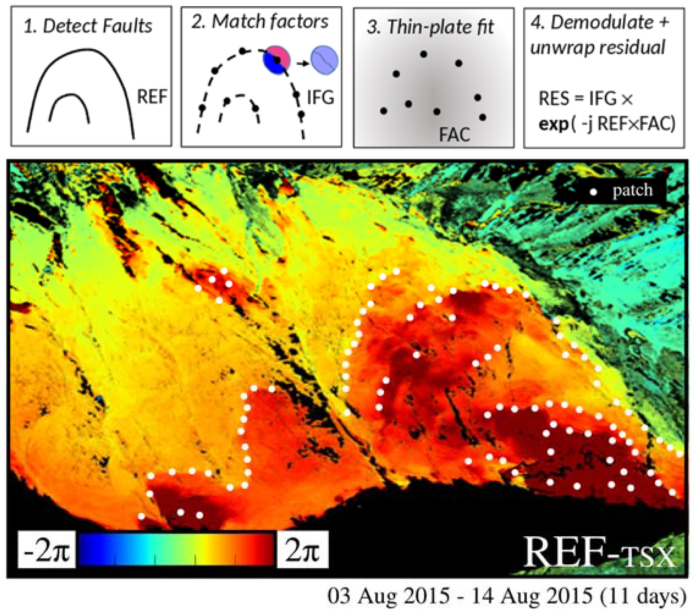
Detect Active Fault Locations. Active fault locations can be mapped robustly and accurately by using a curvature criterion (second-order derivative; minimum threshold on the largest eigenvalue and contrast of eigenvalues of the two-dimensional (2D) Hessian matrix of factor >10) applied to a smoothed version of the reference interferogram. This, or a similar discontinuity detection approach, must be used by the wireframe model, which requires continuous parameterization of each active fault line in its entirety. For the warp demodulation model, it is sufficient for each fault line to be represented by a (generally coarser and irregularly spaced) representative set of points. Such a set can be found by subsampling the output from the described curvature criterion discontinuity detector. This approach was used for the Fels Glacier Slide example (see Section 3.2). Alternatively, it is possible to digitize the point set representing the faults manually on the reference interferogram (as was done for the sensitivity analysis in Section 3.1); this approach may be generally more robust, particularly if a less coherent and high-resolution reference is used.

Step 2

Find Local Match Factors. The reference is matched to the to-be-demodulated interferograms within circular patches straddling the active faults at the pointset locations found in the first step. The radius of the patches is an important parameter of the model whose influence on the accuracy and robustness of the demodulation is discussed later. Optimum multiplicative factors to scale the reference before demodulation are obtained now for each patch by maximizing the (signal-biased) coherence estimate of the residual inside the patch. While this type of match (coherence optimization) essentially minimizes the dynamic range of the coherent phase residual of the patch (incoherent phase noise inside the patch does not change during the optimization and thus does not affect it) it is insensitive to the phase offset between the interferogram and the scaled reference. This is a key feature of our warp demodulation method, which favors spatial smoothness over smallness of the demodulation residual.

Step 3

Thin Plate Spline Fit. The vector of optimum match factors at the point set locations is now interpolated to form a continuous function of the interferogram coordinates using a thin plate spline fit. This function is then multiplied with the reference to warp the latter into an optimum demodulation phase surface for the interferogram. This demodulation phase is then wrapped, and its complex conjugate is multiplied with the to-be-demodulated interferogram to form the residual phase.

Step 4

Unwrap Residual. The residual phase, optimally smooth and slowly varying spatially, is multi-looked and unwrapped using standard Minimum Cost Flow (MCF) techniques [17]. The unwrapped residual is added to the constructed (unwrapped) demodulation phase of step 3 to form the final unwrapped interferogram.

The warp demodulation method has several unique characteristics: (i) as already mentioned, the method is designed to produce a smooth demodulation residual; the mean phase offset for each patch between the reference and the to-be-demodulated interferogram deliberately is not considered in finding the optimum local matching factors; (ii) phase structures inside the patch instead are used for the optimization; primarily, the phase discontinuity along the fault line dissecting the patch is used, but secondarily, the gradients and curvature features of the displacement phase of the landslide lobes are also used. The ability to use this secondary information allows the method to succeed in finding the correct demodulation surface, even if phase aliasing occurs across the fault due to the acceleration of a lobe along its downslope axis. The chosen patch radius plays an important role in how robustly the method delivers on this ability, and this is discussed in Section 3.1, where we present a full parametric sensitivity analysis of the method; (iii) our method relies on approximate stationarity of the phase discontinuities between the reference and the interferogram: significant shifting of active faults leads to artifacts also discussed in Section 3.1. The method biases the local scale factor to zero for a “flat” coherence optimum, which handles the case correctly that when an active fault in the reference is inactive in the interferogram, the resulting residual is smooth. However, for the opposite case where a fault in the interferogram is not present in the reference, the coherence optimization will be insensitive and cannot diminish the signal (residual will remain discontinuous). The wireframe model has the same problem; if new active faults are generated, then the reference needs to be updated to include the new faults as cuts. As there, (iv) the warp demodulation method can be generalized straightforwardly by including several references appropriately spaced temporally and selecting the one close enough in time for each to-be-demodulated interferogram to capture adequately the formation (and cessation) of active faults.

3. Results

In this section, we present results from a sensitivity analysis of the new method, as well as demonstration results using actual data.

Table 2. List of parameters used in Section 3.

Symbol	Description
IFG	To-be-demodulated wrapped interferogram
REF	High-resolution unwrapped reference interferogram
FAC	Thin-plate interpolated warp demodulation factor
RES	Wrapped warp demodulation residual
RES-UNW	Unwrapped warp demodulation residual
UNW	IFG unwrapped through warp demodulation
Δh	Downward shift of the IFG active lobe (with respect to REF); units: pixels
${\mathrm{f}}_{\mathrm{REF}}$	Along-lobe deformation rate in the REF interferogram; units: fringes/lobe
${\mathrm{f}}_{\mathrm{INF}}$	Along-lobe deformation rate in the INF interferogram. units: fringes/lobe
${\Delta }_{\mathrm{f}}$	Difference (between REF and IFG) in the along-lobe deformation rate; units: fringes/lobe
$r$	Demodulation patch radius; units: fraction of the main lobe’s diameter
$\kappa$	Steepness of logistic curve
GAU	Atmospheric phase error surface
σ	Standard deviation of GAU

contains a list of symbols and acronyms used in Section 3. We want to point out explicitly that our warp demodulation method assumes the existence of a reference interferogram of “good quality”, quantified as high coherence and unobscured by layover with an MCF unwrapping result that is correct except for perhaps localized small errors (restricted to the vicinity of a few pixels around minor incoherent areas). Therefore, within the scope of the present study, the effects arising from shortcomings of the reference have not been included in the sensitivity analysis.

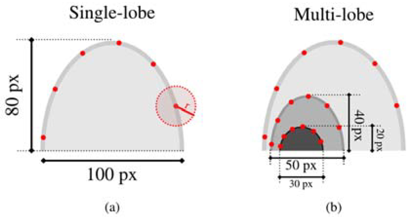
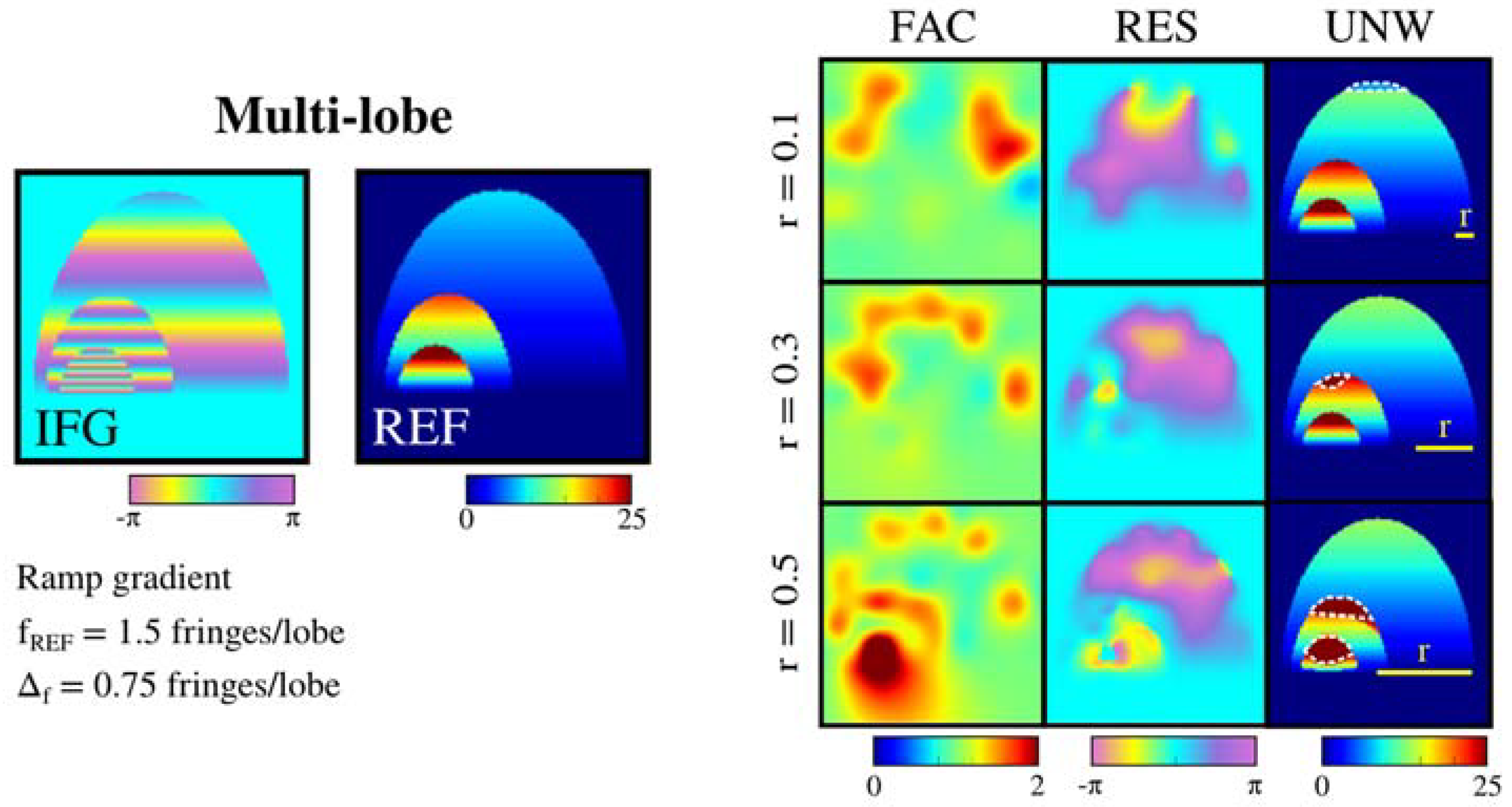
3.1. Sensitivity Analysis with Simulated Data

The warp demodulation method is applied to a dataset of simulated InSAR observations for two different landslide scenarios:

• Single-lobe: the deforming active lobe is modeled by a semi-ellipse (vertical semi-axis of 80 pixels, horizontal axis of 100 pixels, Figure 2a).
• Multi-lobe: three nested semi-elliptical lobes are simulated (see Figure 2b for dimensions).

The goal of this analysis is to assess the robustness and limitations of warp demodulation with respect to the following landslide deformation and/or demodulation parameters (see also Figure 3):

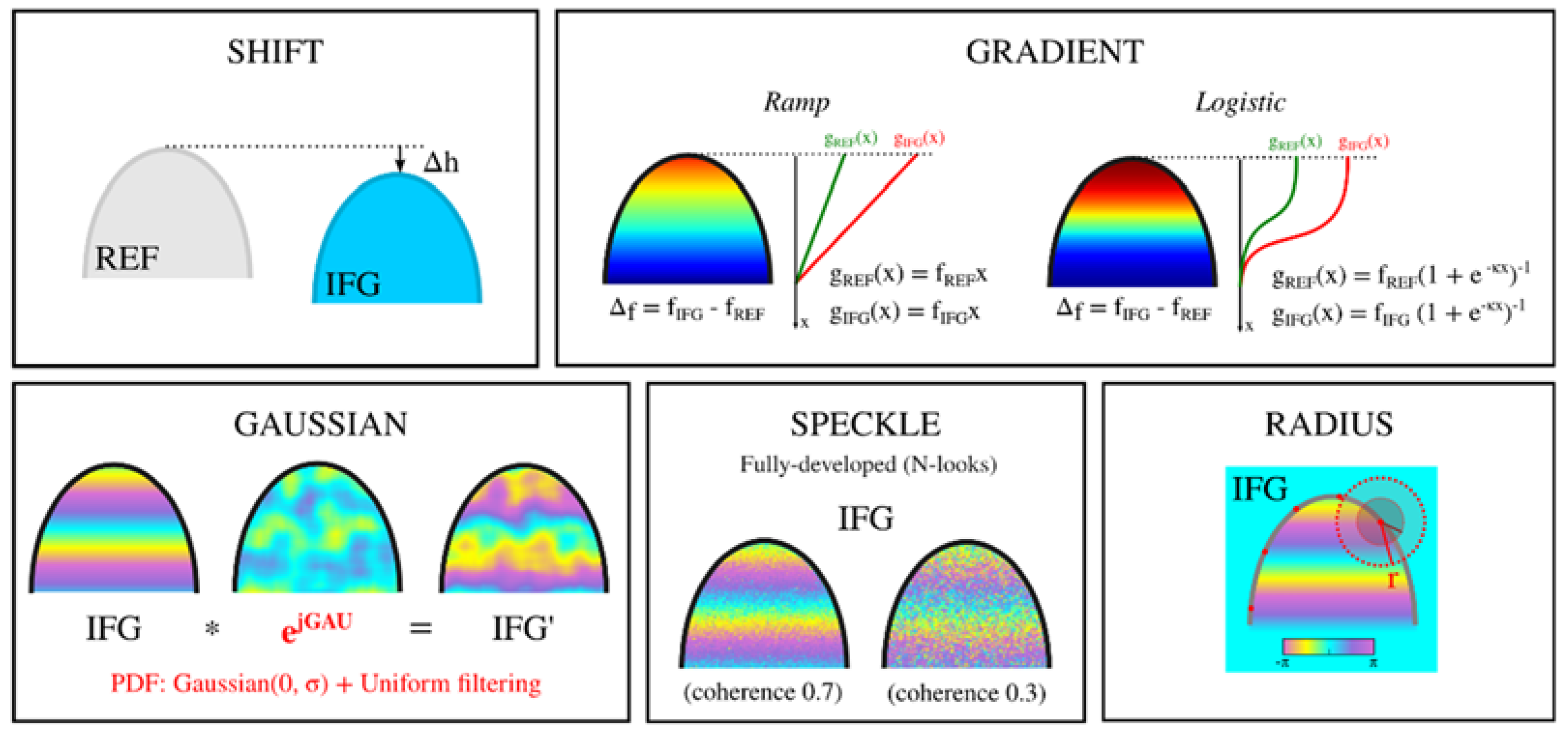
• Downward shift of the to-be-demodulated wrapped interferogram (IFG) active lobe (with respect to high-resolution unwrapped reference interferogram (REF)).
• Along-lobe deformation gradient types (linear or logistic ramp) and deformation rates.
• IFG “disturbances” (i.e., atmospheric and random phase noise (related to speckle)).
• Radius of the demodulation patches $r$ (expressed in a fraction of the main lobe’s diameter).

Table 3. Sensitivity analysis with simulated data. Overview of the simulation experiments and results.

Experiment	Description	Model Parameters		Observations
SHIFT	Robustness against downward shift Δh of the IFG active lobe (with respect to REF) at different REF along-lobe deformation rates ${\mathrm{f}}_{\mathrm{REF}}$	VAR	$\mathsf{\Delta }\mathrm{h}=\left[0,30\right]$ px ${\mathrm{f}}_{\mathrm{REF}}=1, 1.5, 2, 4$ fringes/lobe	RMSE monotonically increasing with Δh RMSE positively associated with ${\mathrm{f}}_{\mathrm{REF}}$
		FIXED	${\Delta }_{\mathrm{f}} =0$ fringes/lobe $r=0.25$ 6 patches Gradient: ramp
GRADIENT	Robustness against along-lobe deformation differences ${\Delta }_{\mathrm{f}}$ between REF and IFG for ramp/logistic along-lobe deformation gradients	VAR	Gradient: ramp/logistic ${\Delta }_{\mathrm{f}}=\left[0, 2\right]$ fringes/lobe ${\mathrm{f}}_{\mathrm{REF}}=1, 1.5, 2, 4$ fringes/lobe $\kappa =2, 4$ (logistic)	RMSE constant until ${\Delta }_{\mathrm{f}}$ = 1 fringe/lobe, then abruptly increasing Ramp (${\Delta }_{\mathrm{f}}$ > 1 fringe/lobe): RMSE negatively associated with ${\mathrm{f}}_{\mathrm{REF}}$
		FIXED	Δh = 0 px $r=0.25$ 6 patches
SPECKLE	IFG affected by fully developed speckle (distribution as in [26])	VAR	Gradient: ramp/logistic ${\Delta }_{\mathrm{f}}=\left[0, 2\right]$ fringes/lobe ${\mathrm{f}}_{\mathrm{REF}}=1, 1.5, 2, 4$ fringes/lobe Coherence = 0.3, 0.5, 0.7	RMSE trend in agreement with GRADIENT RMSE negatively associated with coherence
		FIXED	Δh = 0 px $r=0.25$ 6 patches Number of looks = 5 $\kappa =4$ (logistic)
GAUSSIAN	IFG affected by Gaussian noise (atmosphere-like disturbance)	VAR	Gradient: ramp/logistic ${\Delta }_{\mathrm{f}}=\left[0, 2\right]$ fringes/lobe ${\mathrm{f}}_{\mathrm{REF}}=1, 1.5, 2, 4$ fringes/lobe $\sigma =3, 7, 11$	RMSE trend in agreement with GRADIENT RMSE and $\sigma$ are positively associated
		FIXED	Δh = 0 px $r=0.25$ 6 patches $\kappa =4$ (logistic)
RADIUS	Impact of patch radius $r$ on demodulation performance	VAR	Gradient: ramp/logistic ${\mathrm{f}}_{\mathrm{REF}}=1, 1.5, 2, 4$ fringes/lobe $r=\left[0.1, 0.7\right]$	Single-lobe: RMSE positively associated with $r$ when $r>0.35$ Minimum RMSE when $0.3<r<0.5$ Multi-lobe: Phase artifacts within the secondary lobes as $r$ increases
		FIXED	Δh = 0 px 6 patches ${\Delta }_{\mathrm{f}}=2$ fringes/lobe (ramp, single-lobe) ${\Delta }_{\mathrm{f}}=0.75$ fringes/lobe (ramp, multi-lobe) ${\Delta }_{\mathrm{f}}=0.75$ fringes/lobe (logistic) $\kappa =4$ (logistic)

provides an overview of the experiments and a summary of the simulation results. The most relevant findings of the simulation study are detailed in Section 3.1.1, Section 3.1.2 and Section 3.1.3

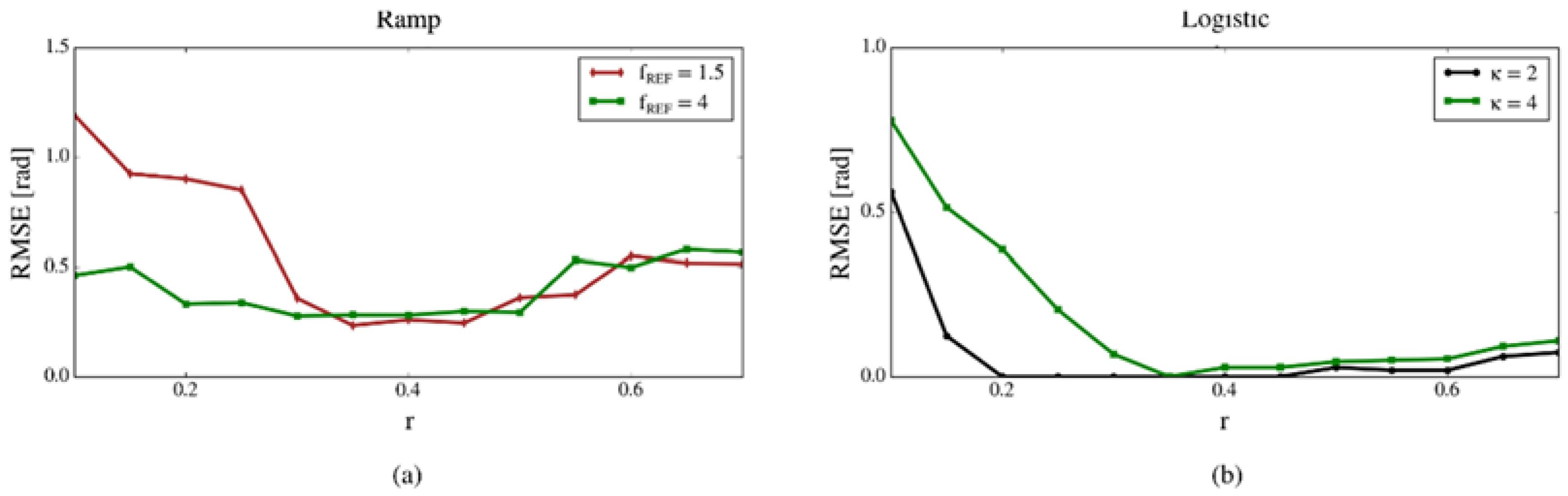
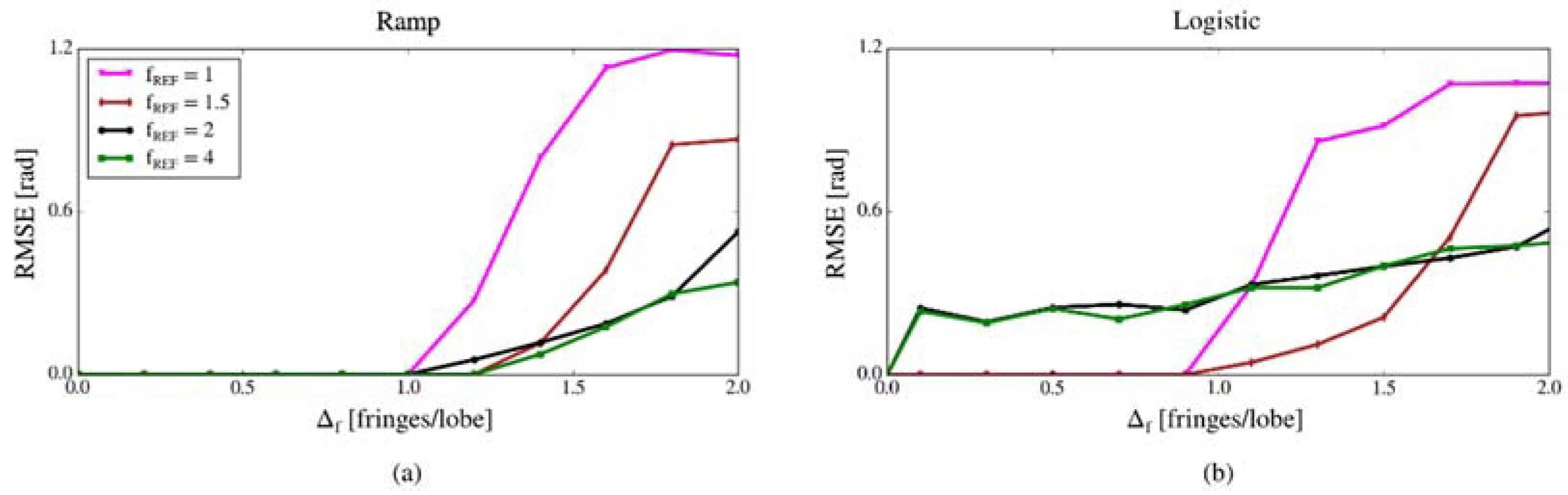
3.1.1. Along-Lobe Deformation Gradients

In Figure 4, the Root-Mean-Square Error (RMSE) of the demodulated unwrapped phase is displayed as a function of the difference (i.e., between REF and IFG) in the along-lobe deformation rate ${\Delta }_{\mathrm{f}}={\mathrm{f}}_{\mathrm{IFG}}-{\mathrm{f}}_{\mathrm{REF}}$ for four different REF along-lobe deformation rates ${\mathrm{f}}_{\mathrm{REF}}$. The warp demodulation method is run using six equally spaced demodulation patches of $r=0.25$ located on the main lobe discontinuity. The statistics are obtained by assuming either a ramp or a logistic along-lobe deformation gradient. In the latter, a curve steepness $\kappa =4$ is imposed.

Ramp gradient: The RMSE remains substantially insensitive to ${\mathrm{f}}_{\mathrm{REF}}$ and is approximately equal to zero if ${\Delta }_{\mathrm{f}}$ < 1 fringe/lobe. Above this threshold, the RMSE tends to increase with ${\Delta }_{\mathrm{f}}$ until the latter reaches approximately 1.6–1.8 fringes/lobe, then the two quantities become again uncorrelated. Such an increase is markedly abrupt for ${\mathrm{f}}_{\mathrm{REF}}=1$ fringe/lobe (from 0 to 0.96 rad as ${\Delta }_{\mathrm{f}}$ increases from 1 to 1.5 fringes/lobe).

For ${\Delta }_{\mathrm{f}}$ values bigger than 1 fringe/lobe, the RMSE is also negatively associated with ${\mathrm{f}}_{\mathrm{REF}}$. For instance, RMSE at ${\Delta }_{\mathrm{f}}=1.5$ fringes/lobe is seen to increase by 0.85 rad in response to a ${\mathrm{f}}_{\mathrm{REF}}$ reduction by 50%.

Logistic gradient: If ${\mathrm{f}}_{\mathrm{REF}}=1$ fringes/lobe, the RMSE remains approximately equal to zero until approximately ${\Delta }_{\mathrm{f}}$ = 1 fringe/lobe, when it abruptly increases, reaching a maximum of 1.05 rad at ${\Delta }_{\mathrm{f}}$ = 1.7 fringes/lobe. The same behavior with ${\Delta }_{\mathrm{f}}$, although with a less abrupt increase, is also found for ${\mathrm{f}}_{\mathrm{REF}}=1.5$ fringes/lobe. If $2<{\mathrm{f}}_{\mathrm{REF}}<4$ fringes/lobe, the RMSE shows a positive association with ${\Delta }_{\mathrm{f}}$ (Pearson’s correlation coefficient $R=0.93$); in this case, the statistics appear substantially insensitive to ${\mathrm{f}}_{\mathrm{REF}}$ and range from a minimum of 0.2 rad (at ${\Delta }_{\mathrm{f}}$ = 0.3 fringes/lobe) to a maximum of 0.5 rad (at ${\Delta }_{\mathrm{f}}$ = 1.9 fringes/lobe).

3.1.2. Effect of Atmosphere-Like Disturbances

We simulated a two-dimensional atmospheric phase error surface (GAU) that shares the spatial characteristics of the dynamic atmosphere. GAU is assumed to be zero-mean Gaussian-distributed (with standard deviation $\mathsf{\sigma }$) and is smoothed via an 11-pixel uniform filter. The to-be-demodulated interferogram IFG’ now has the form:

$$\mathrm{IF}{\mathrm{G}}^{\prime }=\mathrm{IFG}·{\mathrm{e}}^{\mathrm{j}\mathrm{GAU}}$$

(1)

In

Table 4. Sensitivity analysis with simulated data, effect of atmosphere-like disturbances. RMSE (in radians) of the demodulated unwrapped phase at three different $\mathit{\sigma }$ values (ramp gradient).

		$\mathit{\sigma }=\mathbf{3}$	$\mathit{\sigma }=\mathbf{7}$	$\mathit{\sigma }=\mathbf{11}$
${\Delta }_{\mathbf{f}}$= 0.5	${\mathbf{f}}_{\mathbf{REF}}=\mathbf{1}$	0.181	0.417	0.670
	${\mathbf{f}}_{\mathbf{REF}}=\mathbf{4}$	0.180	0.433	0.675
${\Delta }_{\mathbf{f}}$= 1.0	${\mathbf{f}}_{\mathbf{REF}}=\mathbf{1}$	0.179	0.423	0.674
	${\mathbf{f}}_{\mathbf{REF}}=\mathbf{4}$	0.178	0.432	0.683
${\Delta }_{\mathbf{f}}$= 1.5	${\mathbf{f}}_{\mathbf{REF}}=\mathbf{1}$	1.087	1.185	1.345
	${\mathbf{f}}_{\mathbf{REF}}=\mathbf{4}$	0.260	0.467	0.719

and

Table 5. Sensitivity analysis with simulated data, effect of atmosphere-like disturbances. RMSE (in radians) of the demodulated unwrapped phase at three different $\mathit{\sigma }$ values (logistic gradient).

		$\mathit{\sigma }=\mathbf{3}$	$\mathit{\sigma }=\mathbf{7}$	$\mathit{\sigma }=\mathbf{11}$
${\Delta }_{\mathbf{f}}$= 0.5	${\mathbf{f}}_{\mathbf{REF}}=\mathbf{1}$	0.180	0.431	0.667
	${\mathbf{f}}_{\mathbf{REF}}=\mathbf{4}$	0.308	0.624	0.832
${\Delta }_{\mathbf{f}}$= 1.0	${\mathbf{f}}_{\mathbf{REF}}=\mathbf{1}$	0.181	0.451	0.705
	${\mathbf{f}}_{\mathbf{REF}}=\mathbf{4}$	0.477	0.651	0.866
${\Delta }_{\mathbf{f}}$= 1.5	${\mathbf{f}}_{\mathbf{REF}}=\mathbf{1}$	1.161	1.257	1.414
	${\mathbf{f}}_{\mathbf{REF}}=\mathbf{4}$	0.528	0.692	0.905

, we reported the mean RMSE of the demodulated unwrapped phase computed for a population of 50 randomly generated IFG’ observations at three different $\sigma$ values. The statistics are obtained by assuming either a ramp or a logistic ($\kappa =4$) along-lobe deformation gradient.

The mean RMSE shows a trend with ${\Delta }_{\mathrm{f}}$ that is in agreement with the results of Section 3.1.1 (constant until ${\Delta }_{\mathrm{f}}$ = 1 fringe/lobe, then abruptly increasing). Compared to Section 3.1.1, all RMSE measurements of Table 4 and Table 5 are now affected by a positive offset that is positively associated with $\sigma$ (e.g., compared to the case where $\sigma =3$, the RMSE at $\sigma =11$ is on average 0.44 rad greater).

3.1.3. Impact of the Demodulation Patch Radius

To assess the performance of the warp demodulation approach with respect to the radius of the demodulation patches $r$, the RMSE of the demodulated unwrapped phase is plotted against $r$ when either a ramp or a logistic deformation gradient is imposed (Figure 5a,b, respectively). All simulations are performed using six patches located on the main lobe discontinuity.

Ramp gradient (${\Delta }_f=2$): When $r<0.35$, the RMSE is consistently larger at ${\mathrm{f}}_{\mathrm{REF}}=1.5$ fringes/lobe than at ${\mathrm{f}}_{\mathrm{REF}}=4$ fringes/lobe (maximum difference of 0.72 rad at $r=0.1$). Above this threshold, the RMSE becomes insensitive to ${\mathrm{f}}_{\mathrm{REF}}$ and positively associated with $r$ ($R=0.93$ at ${\mathrm{f}}_{\mathrm{REF}}=1.5$ fringes/lobe; $R=0.9$ at ${\mathrm{f}}_{\mathrm{REF}}=4$ fringes/lobe). The smallest RMSE (0.25 rad) is observed when $0.3<r<0.5$.

Logistic gradient (${\Delta }_f =0.75, f_{REF}=4$): The RMSE is consistently smaller at $\kappa =2$ than $\kappa =4$ and is seen to decrease with increasing $r$ when the latter is below 0.2 ($\kappa =2$) or 0.35 ($\kappa =4$). Above these thresholds, the RMSE remains consistently below 0.1 rad and positively associated with $r$ ($R=0.84$ at $\kappa =2$; $R=0.96$ at $\kappa =4$).

The warp demodulation is also applied to a multi-lobe scenario with ${\Delta }_{\mathrm{f}}=0.75$ fringes/lobe and ${\mathrm{f}}_{\mathrm{REF}}=1.5$ fringes/lobe (ramp gradient). As shown in Figure 6, a small radius $r=0.1$ results in localized phase errors within the main lobe (RMSE = 0.206 rad). When $0.3\le r\le 0.5$, the phase gradient along the main lobe is accurately reconstructed. However, a number of phase artifacts within the secondary lobes can now be observed. The number of artifacts, and hence the RMSE, appear to increase with increasing $r$ ($r=0.3:$ RMSE = 0.181 rad, $r=0.5:$ RMSE = 1.318 rad).

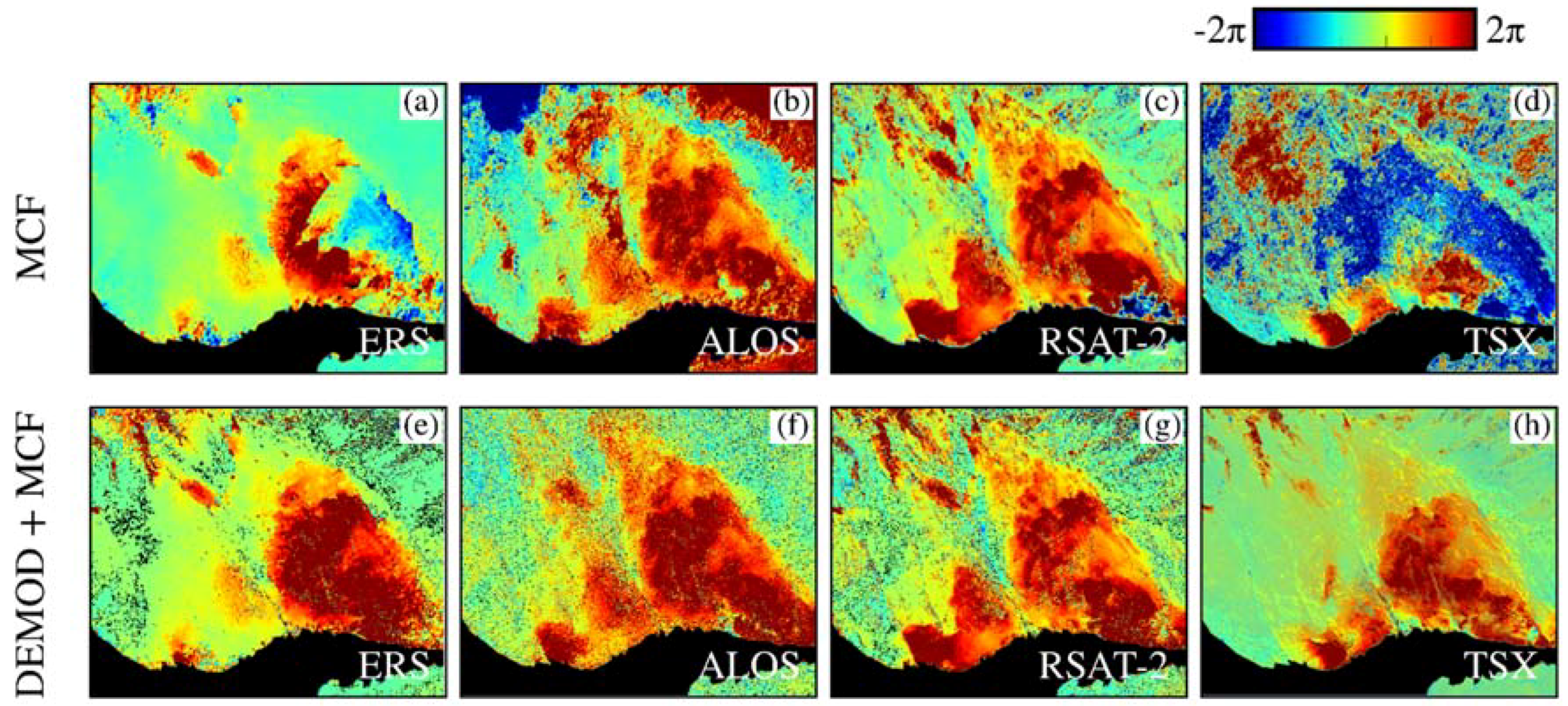
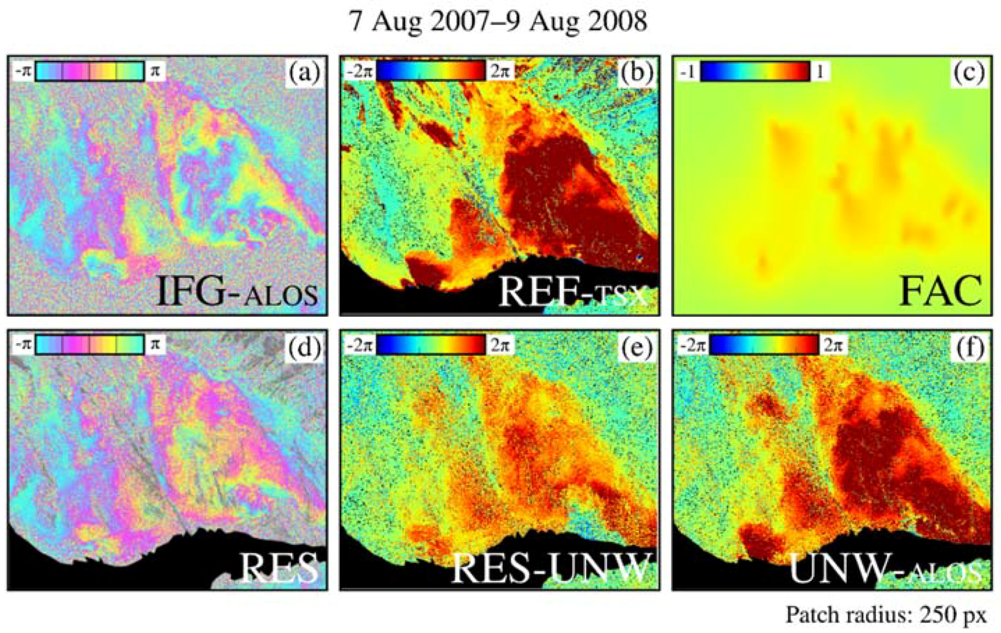
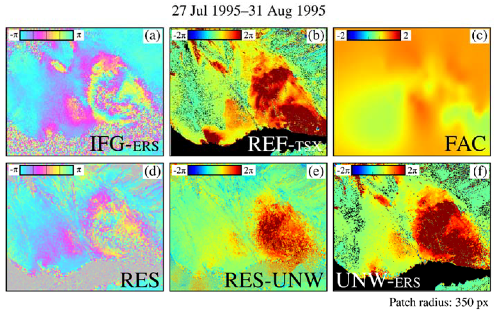
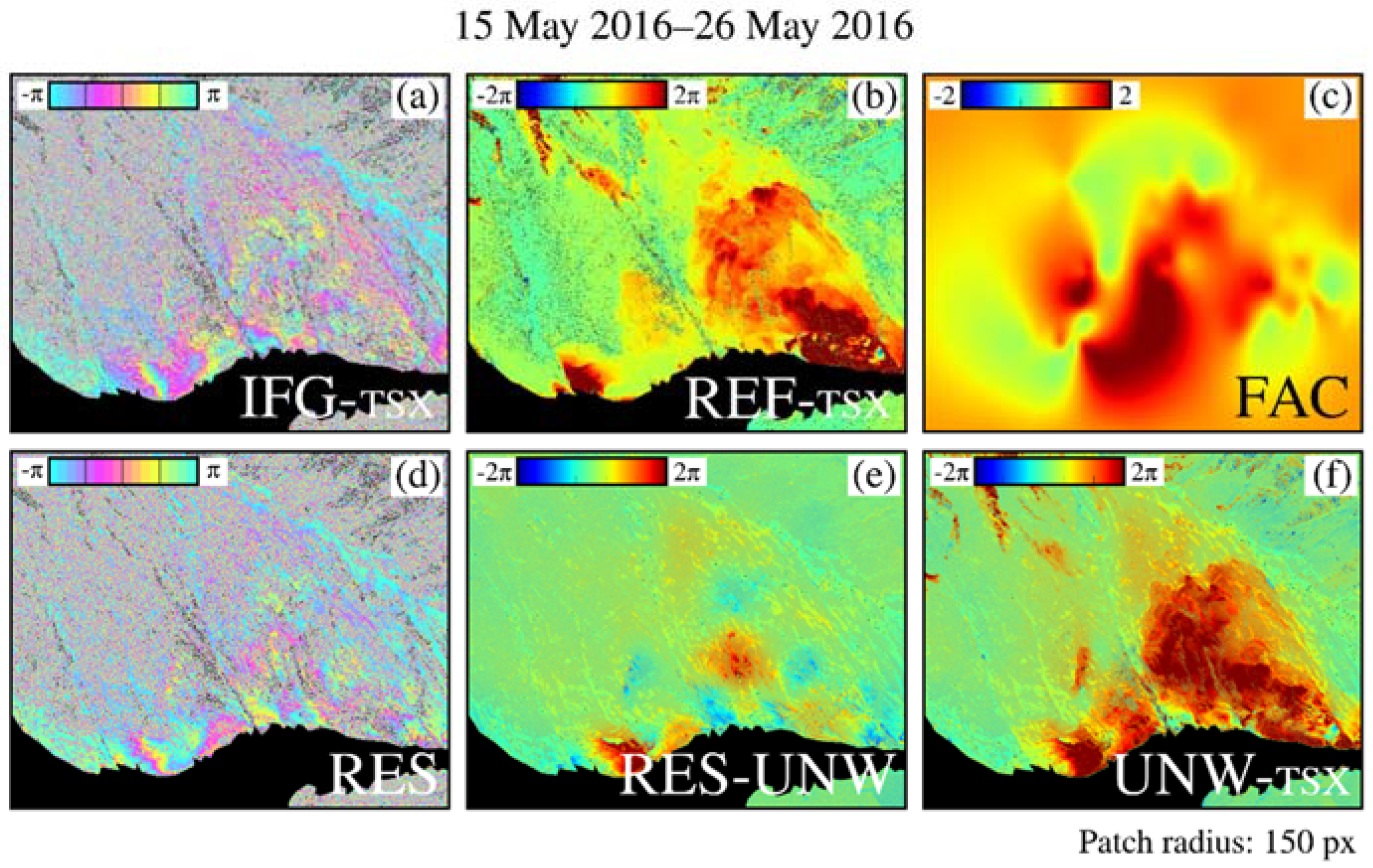
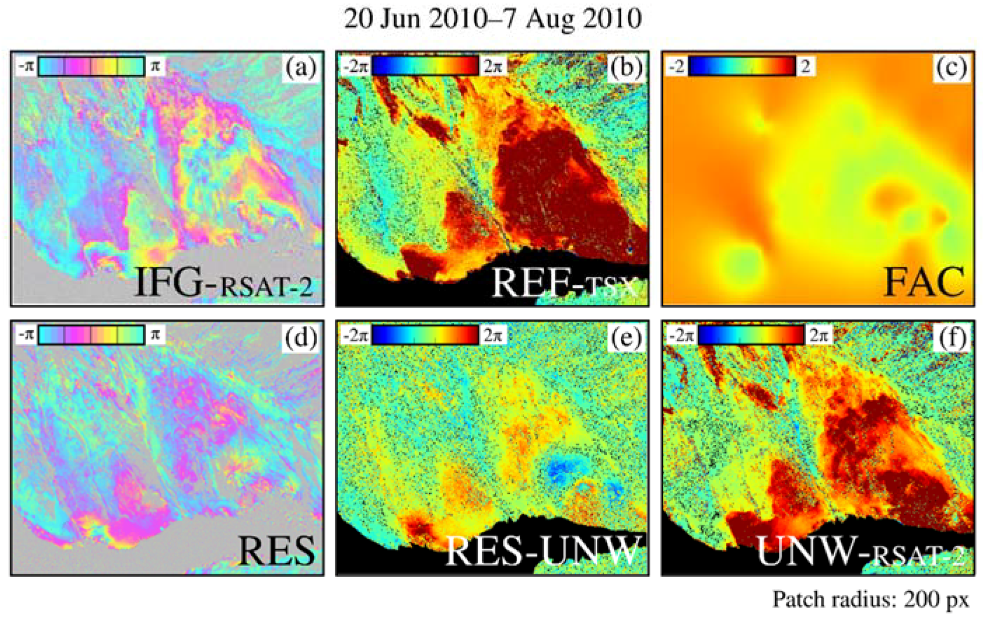
3.2. Real Data Example: Fels Glacier Slide

In the following, we give a demonstration of the warp demodulation method for a representative large, complex landslide test site, the Fels Glacier Slide in Alaska. The Fels Glacier Slide [27] occupies an instable, south-facing slope above and immediately adjacent to the lower Fels Glacier. The Fels Slide is about 3 km from the Alaska Pipeline corridor to the west and about 2 km from the Denali Fault to the south; earthquakes generated by the Denali Fault, such as the M7.9 one in November 2002, significantly affect the slide dynamics. Other obvious drivers of the dynamics of the slide are meteorology (mostly snow melt and rain) and the ongoing recession of the Fels Glacier, which additionally destabilizes the toe of the slide. On the surface, the deforming area of the slide is about 3 km wide and has approximate fall line and elevation extents of 2 km and 600 m, respectively. The mechanism of the deformation is a deep-seated (depth and shape of the failure plane unknown) gravitational mass deformation forming two large lobes separated east–west by a central dissecting gully. Overlain onto these two deep-seated main lobes are several smaller more surficial deforming lobes that cause strong discontinuities in the deformation field where the surface ruptures along extensive downward curving arcuate fissures. While the deformation is classified as creep-type, movement amounts can easily exceed 30 cm per year for the fastest areas of the slide.

As inputs to our demodulation method, to construct the high-resolution reference “model” we use a TSX-ST image pair 3–14 August 2015 (0.6 m spatial resolution; shown in Figure 1), and for the to-be-demodulated lower resolution interferograms, we have selected three representative examples, one each from ERS, ALOS-1, and RADARSAT-2 capturing different resolution (30 m, 15 m, and 3 m, respectively), seasonal and annual separation, coherence conditions, and interferogram periods with respect to the reference (

Table 6. Synthetic aperture radar (SAR) datasets used to test the warp demodulation method.

Sensor	Resolution (m)	Temp. Baseline	Incidence Angle (deg)	Track Angle (deg)
TSX-ST	0.6	11 days	41.3	−169.0
RADARSAT-2	3	48 days	44.0	−171.0
ALOS-1	15	368 days	38.8	−168.7
ERS	30	35 days	23.3	−164.3

). The TSX-ST reference is unwrapped using MCF and re-projected to the line-of-sights of the respective other sensors. The re-projection assumes an approximate motion direction following the average fall line as derived from a spatially smoothed version (500 m scale) of the external DSM used for the topographic corrections and is generally robust due to the similarity of acquisition geometries of the different sensors. Track angles in Table 6 are very similar, as expected for space-borne data of the same orbit direction; look angles are more different but still only vary by less than 20 degrees, which for only moderately rugged topography (as is the case for the Fels Glacier Slide) does not lead to stark layover/shadow contrasts for the different incidence angles, guaranteeing a smooth re-projection map. After re-projection of the template, the warp demodulation method is then applied as introduced in Section 2 and analyzed in Section 3.1.

Standard MCF unwrapping (using coherence costs and masking areas with coherence below 0.3) results of four selected test interferograms over the Fels Glacier Slide are shown in Figure 7, subfigures (a)–(d). For easy comparison, subfigures (e)–(h) of Figure 7 show the final corresponding warp demodulation results presented in detail in Figure 8, Figure 9, Figure 10 and Figure 11 (lower right panels). Problems from erroneous branch cuts made by the MCF algorithm are immediately apparent for both the ERS case (within the main lobe, Figure 7a) and most strikingly for the TSX case (Figure 7d). For the ALOS-1 and RSAT-2 cases (Figure 7b,c, respectively), MCF performs better; however, more localized branchcut problems are still easily identifiable.

Respective warp demodulation results for the same test sites are presented in Figure 8, Figure 9, Figure 10 and Figure 11 (as just stated the unwrapped interferogram (UNW) of the lower right sub-figures are also shown in Figure 7e–h). The test case of Figure 8 (TSX-ST 2016) selects a partially incoherent interferogram with strong seasonal deformation contrast but with the same resolution and close in absolute time to the reference template (TSX-ST 2015). The figure order of the remaining three test cases (RADARSAT-2 2010, ALOS-1 2007/2008, and ERS 1995) aligns with going further into the past of the slide deformation, as well as towards coarser resolution. Each figure has six panels, which starting in the upper-left and going clockwise represent the following: (a) IFG, the to-be-demodulated interferogram; (b) REF, the line-of-sight re-projected unwrapped reference; (c) FAC, the warp demodulation factor map; (d) RES, the wrapped demodulated interferogram; (e) RES-UNW, the unwrapped demodulated interferogram, and (f) UNW, the final interferogram unwrapped through warp demodulation. Note that REF appears different in each figure, as creating the reference template involves line-of-sight re-projections of the (same) TerraSAR-X interferometric pair into the (all different) viewing geometries of the other sensors. The choice of demodulation patch sizes reflects our reasoning on the different resolutions and atmospheric and random noise phase error levels of the different sensors. For example, ERS has the largest radius (350 pixels); ERS has comparable atmospheric error to RADARSAT-2, but its random noise is higher due to factor 10 lower resolution. ALOS-1 (patch radius 250 pixels), covering one entire year, has random noise only slightly lower than ERS over one month, but tropospheric atmospheric noise levels in L-band are expected to be much lower than for ERS. Due to its considerably high-resolution, the RADARSAT-2 patch radius is the smallest (200 pixels).

The findings from the real data experiments indicate that, unlike standard MCF unwrapping (Figure 7d), the warp demodulation method performs creditably over the TSX-ST interferogram of May 2016 (Figure 8) despite the extensive (around 50 percent of area) low coherence areas of the original interferogram. Further, the findings confirm (most obvious in the 48-day C-band interferogram of Figure 9) that our method can handle significant aliasing in IFG that “hides” active discontinuities through a near integer 2-pi phase ambiguity; warp demodulation still finds the correct FAC values across these discontinuities by matching between IFG and REF the spatial texture of the phase surfaces on both sides of the fault. RES in Figure 9d is smooth and within a single fringe, which indicates a successful warp demodulation.

Also, for the other two cases (Figure 10 and Figure 11) involving sensors with considerably coarser resolution, our method still performs satisfactorily in producing phase residuals that are both spatially smooth and sufficiently small to reconstruct the unwrapped phase of the test interferograms. Reconstruction is not perfect, firstly due to the error sources identified in Section 3.1 (e.g., migration and introduction of deformation discontinuities), plus a few additional ones (such as small unwrapping errors in the reference in some small layover regions but particularly in the fast-moving area where the eastern lobe meets the Fels Glacier). Errors in the reconstruction are by and large limited to this fastest moving part of the slide (most visible in Figure 10e, the unwrapped residual of the ALOS-1 case), where the reference likely would also not be representative due to separation in time even in the absence of any phase unwrapping errors.

4. Discussion

The sensitivity analysis of the warp demodulation method in Section 3.1 using synthetic data identifies a number of error sources assuming a perfect reference. Our method, for obvious reasons, cannot reconstruct areas where the reference does not exist. However, in areas where the high-resolution interferogram used to generate the demodulation reference is of high quality and has been correctly unwrapped, our method is robust with respect to almost all potential error sources; the ones analyzed in Section 3.1 and others associated with the described processing steps, such as the re-projection of the unwrapped reference to the line-of-sight of the to-be-demodulated interferogram. Of particular interest is the ability of our method to recover the unwrapped phase correctly across a lobe discontinuity, even if the phase has several wraps when followed along the discontinuity delineating the lobe. This ability depends on the presence of a significantly strong spatial texture (local gradient or curvature) in the phase that can be matched between reference and to-be-demodulated interferogram to break the two-pi ambiguity of the phase jump across the discontinuity. To match spatial textures robustly, a large enough patch size is critical. However, a very large size can also cause patches to overlap with multiple discontinuities, where they are closely spaced, which prevents a smooth residual should differential deformation changes occur for the different discontinuities with respect to the reference. The analysis in Section 3.1.3 revealed quantitatively how patch size trades off quantitatively for realistic lobe configurations. Our warp demodulation method is generally robust for a range of patch sizes between a half and a fifth of the main lobe diameter. An enhanced future version of our method will use an adaptive patch size that takes the variable spacing of phase discontinuities (slide faults) into account to combine the increase in robustness with patch size with preserved high-resolution where several discontinuities are nested close together.

A noteworthy exception to the generally robust behavior of the warp demodulation method is when the reference gets “out of date” (i.e., the number of discontinuities of the deformation field identified in the reference does not match that in the to-be-demodulated interferogram (this can be considered a more extreme case of the subtle shifting of discontinuities included in the analysis of Section 3.1)). For the case of a qualitative mismatch of discontinuities, where either (i) an extra discontinuity or (ii) a discontinuity identified in the reference is not active in the interferogram, there is a pronounced asymmetry. For case (ii), the warp factor will down-scale the reference locally at the inactive discontinuity; the warp modulation method is robust to this case (=smooth residual). However, for case (i), the residual will be insensitive to the warp factor and the residual will be locally discontinuous. Thus, if too many discontinuities are missing in the reference and there are additional high-resolution datasets available closer in time, then a new reference should be constructed and used instead.

As mentioned before, our method is easily generalized to several references and can also be used iteratively (i.e., successfully warp-demodulated interferograms can themselves be used as reference). A full generalization of our method to a wireframe representation in space and time is considered as a next step. For a slide with a deep, historic InSAR dataset, this would then include an explicit parameterization of the spatio-temporal pattern of the active faults of the landslide, including formation, migration, and healing of faults. The patch measurements carried out with our original warp demodulation concept presented in Section 2 could be used to make the explicit fault parametrization converge. Once found, the explicit fault parametrization can then be used to demodulate/unwrap the full time series of interferograms (as discontinuous aliased phase surfaces) in a single optimization step (as per the original wireframe concept).

Besides the robustness of the method, the interpretation of the two results per interferogram (i) warp factor map and (ii) residual phase map is also of interest for discussion. As our method targets smoothness but not necessarily the overall smallest size of the phase residual after demodulation, neither the residual, nor the warp factor maps can be easily interpreted quantitatively as a measure of bulk slide activity relative to that of the reference. Qualitatively, a smooth residual shows persistence of the fault pattern between the interferogram and the reference. Also, a factor map in the 1-range plus a small residual indicates that the deformation field of interferogram and the reference are very similar. However, beyond that—despite obviously containing important information about the (temporal) changes of the slide dynamics—the interpretation of the pair residual/warp factor map is complex. The studying of a variety of real data examples, such as the ones in Figure 8, Figure 9, Figure 10 and Figure 11, has revealed that the warp factor difference forms one measured change in the shallow (discontinues) deformation field of the slide, while the size of the residual indicates a change in the deep deformation pattern between the interferogram and the reference. More experiments with simulated data are planned to understand this connection more quantitatively.

5. Conclusions

We have developed a new demodulation method (warp demodulation) capable of producing smooth phase residuals to improve the phase unwrapping performance for older, lower resolution, aliased interferograms of complex, multi-lobed, discontinuous landslide deformation. Warp demodulation hinges on the identification of the discontinuity (active fault) pattern on the slide from a high-resolution interferogram, as well as a reference template constructed from the same high-resolution interferogram to match locally the older, coarser interferograms—TerraSAR-X staring spotlight mode (TSX-ST) was found to be exceptionally well suited for this purpose.

A comprehensive sensitivity analysis found the warp demodulation method to be accurate and reasonably robust for all investigated sources. To demonstrate our method, we presented results from three data sets of increasingly coarser resolution and distant in time from the TSX-ST reference. Performance was convincing in all three cases, showing that current high-resolution InSAR and our method can retrieve value from older, low-resolution data that cannot be processed on their own due to low coherence and aliasing, which is useful for the historic analysis of landslide dynamics.

References

1. Rosen, P.A.; Hensley, S.; Joughin, I.R.; Li, F.K.; Madsen, S.N.; Rodriguez, E.; Goldstein, R. Synthetic aperture radar interferometry. Proc. IEEE 2000, 88, 333–382. [Google Scholar] [CrossRef] [Green Version]
2. Bamler, R.; Hartl, P. Synthetic aperture radar interferometry. Inverse Probl. 1998, 14, R1. [Google Scholar] [CrossRef]
3. Strozzi, T.; Farina, P.; Corsini, A.; Ambrosi, C.; Thüring, M.; Zilger, J.; Wiesmann, A.; Wegmüller, U.; Werner, C. Survey and monitoring of landslide displacements by means of L-band satellite SAR interferometry. Landslides 2005, 2, 193–201. [Google Scholar] [CrossRef]
4. Kimura, H.; Yamaguchi, Y. Detection of landslide areas using satellite radar interferometry. Photogramm. Eng. Remote Sens. 2000, 66, 337–344. [Google Scholar]
5. Rott, H.; Scheuchl, B.; Siegel, A.; Grasemann, B. Monitoring very slow slope movements by means of SAR interferometry: A case study from a mass waste above a reservoir in the Otztal Alps, Austria. Geophys. Res. Lett. 1999, 26, 1629–1632. [Google Scholar] [CrossRef]
6. Berardino, P.; Fornaro, G.; Lanari, R.; Sansosti, E. A new algorithm for surface deformation monitoring based on small baseline differential SAR interferograms. IEEE Trans. Geosci. Remote Sens. 2002, 40, 2375–2383. [Google Scholar] [CrossRef]
7. Berardino, P.; Costantini, M.; Franceschetti, G.; Iodice, A.; Pietranera, L.; Rizzo, V. Use of differential SAR interferometry in monitoring and modeling large slope instability at Maratea (Basilicata, Italy). Eng. Geol. 2003, 68, 31–51. [Google Scholar] [CrossRef]
8. Lanari, R.; Casu, F.; Manzo, M.; Zeni, G.; Berardino, P.; Manunta, M.; Pepe, A. An overview of the Small Baseline Subset Algorithm: A DInSAR technique for surface deformation analysis. Pure Appl. Geophys. 2007, 164, 637–661. [Google Scholar] [CrossRef]
9. Rabus, B.T.; Ghuman, P.S. A simple robust two-scale phase component inversion scheme for persistent scatterer interferometry (dual-scale PSI). Can. J. Remote Sens. 2009, 35, 399–410. [Google Scholar] [CrossRef]
10. Ferretti, A.; Prati, C.; Rocca, F. Permanent scatterers in SAR interferometry. IEEE Trans. Geosci. Remote Sens. 2001, 39, 8–20. [Google Scholar] [CrossRef] [Green Version]
11. Colesanti, C.; Ferretti, A.; Novali, F.; Prati, C.; Rocca, F. SAR monitoring of progressive and seasonal ground deformation using the permanent scatterers technique. IEEE Trans. Geosci. Remote Sens. 2003, 41, 1685–1701. [Google Scholar] [CrossRef]
12. Hilley, G.E.; Bürgmann, R.; Ferretti, A.; Novali, F.; Rocca, F. Dynamics of slow-moving landslides from permanent scatterer analysis. Science 2004, 304, 1952–1955. [Google Scholar] [CrossRef] [PubMed]
13. Ferretti, A.; Fumagalli, A.; Novali, F.; Prati, C.; Rocca, F.; Rucci, A. A new algorithm for processing interferometric data-stacks: SqueeSAR. IEEE Trans. Geosci. Remote Sens. 2011, 49, 3460–3470. [Google Scholar] [CrossRef]
14. Eppler, J.; Rabus, B. Monitoring urban infrastructure with an adaptive multilooking InSAR technique. In Proceedings of the FRINGE 2011, Frascati, Italy, 19–23 September 2011. [Google Scholar]
15. Rabus, B.; Eppler, J.; Sharma, J.; Busler, J. Tunnel Monitoring with an Advanced InSAR Technique. Proc. SPIE 2012, 8361, 83611F. [Google Scholar]
16. Costantini, M.; Malvarosa, F.; Minati, F.; Pietranera, L.; Milillo, G. A three-dimensional phase unwrapping algorithm for processing of multitemporal SAR interferometric measurements. In Proceedings of the IEEE International Geoscience and Remote Sensing Symposium, Toronto, ON, Canada, 24–28 June 2002; Volume 3, pp. 1741–1743. [Google Scholar]
17. Costantini, M. A novel phase unwrapping method based on network programming. IEEE Trans. Geosci. Remote Sens. 1998, 36, 813–821. [Google Scholar] [CrossRef]
18. Van Zyl, J.J. The Shuttle Radar Topography Mission (SRTM): A breakthrough in remote sensing of topography. Acta Astronaut. 2001, 48, 559–565. [Google Scholar] [CrossRef]
19. Krieger, G.; Moreira, A.; Fiedler, H.; Hajnsek, I.; Werner, M.; Younis, M.; Zink, M. TanDEM-X: A satellite formation for high-resolution SAR interferometry. IEEE Trans. Geosci. Remote Sens. 2007, 45, 3317–3341. [Google Scholar] [CrossRef] [Green Version]
20. Stramondo, S.; Moro, M.; Tolomei, C.; Cinti, F.R.; Doumaz, F. InSAR surface displacement field and fault modelling for the 2003 Bam earthquake (southeastern Iran). J. Geodyn. 2005, 40, 347–353. [Google Scholar] [CrossRef]
21. Lu, Z.; Dzurisin, D.; Biggs, J.; Wicks, C.; McNutt, S. Ground surface deformation patterns, magma supply, and magma storage at Okmok volcano, Alaska, from InSAR analysis: 1. Intereruption deformation, 1997–2008. J. Geophys. Res. Solid Earth 2010, 115. [Google Scholar] [CrossRef] [Green Version]
22. Woo, K.S.; Eberhardt, E.; Rabus, B.; Stead, D.; Vyazmensky, A. Integration of field characterisation, mine production and InSAR monitoring data to constrain and calibrate 3-D numerical modelling of block caving-induced subsidence. Int. J. Rock Mech. Min. Sci. 2012, 53, 166–178. [Google Scholar] [CrossRef]
23. Carrara, W.G.; Goodman, R.S.; Majewski, R.M. Spotlight Synthetic Aperture Radar: Signal Processing Algorithms; Artech House: Norwood, MA, USA, 1995. [Google Scholar]
24. Mittermayer, J.; Wollstadt, S.; Prats-Iraola, P.; Scheiber, R. The TerraSAR-X staring spotlight mode concept. IEEE Trans. Geosci. Remote Sens. 2014, 52, 3695–3706. [Google Scholar] [CrossRef]
25. Bozdagi, G.; Tekalp, A.M.; Onural, L. 3-D motion estimation and wireframe adaptation including photometric effects for model-based coding of facial image sequences. IEEE Trans. Circuits Syst. Video Technol. 1994, 4, 246–256. [Google Scholar] [CrossRef] [Green Version]
26. Lee, J.S.; Pottier, E. Polarimetric Radar Imaging: From Basics to Applications; CRC Press: Boca Raton, FL, USA, 2009. [Google Scholar]
27. Newman, S.D. Deep-Seated Gravitational Slope Deformations near the Trans-Alaska Pipeline, East-Central Alaska Range. Master’s Thesis, Simon Fraser University, Burnaby, BC, Canada, 2013. [Google Scholar]
Figure 1. Top: the four steps of the warp demodulation method; IFG: to-be-demodulated wrapped interferogram; REF: high-resolution unwrapped reference interferogram; FAC: interpolated factor map; and RES: wrapped residual. Bottom: real data example of reference interferogram (TerraSAR-X Staring Spotlight, 0.6 m ground resolution), Fels Glacier Slide, Alaska.
Remotesensing 10 00995 g001
Figure 2. Sensitivity analysis with simulated data. Schematic depiction of the two simulated landslide scenarios: (a) single-lobe (semi-ellipse) and (b) multi-lobe (three nested semi-ellipses). The red dots identify the location of the demodulation patches (of radius r ).
Remotesensing 10 00995 g002
Figure 3. Sensitivity analysis with simulated data. Schematic depiction of the simulation experiments. SHIFT: robustness of the warp demodulation method against downward shifts Δh of the IFG active lobe; GRADIENT: algorithm sensitivity to along-lobe deformation differences Δ f between REF and IFG for ramp/logistic deformation gradients; GAUSSIAN: IFG affected by Gaussian noise; SPECKLE: IFG affected by fully developed speckle; RADIUS: Impact of patch radius r on demodulation performance.
Remotesensing 10 00995 g003
Figure 4. Sensitivity analysis with simulated data, algorithm robustness against along-lobe deformation differences between REF and IFG. RMSE of the demodulated unwrapped phase as a function of the difference in the along-lobe deformation rate Δ f = f IFG f REF for four different REFs along-lobe deformation rates f REF . The statistics are obtained by assuming (a) a ramp along-lobe deformation gradient or (b) a logistic gradient (curve steepness κ = 4 ).
Remotesensing 10 00995 g004
Figure 5. Sensitivity analysis with simulated data, impact of the demodulation patch radius r on the algorithm performance. RMSE of the demodulated unwrapped phase as a function of r . (a) Ramp gradient, Δ f = 2 fringes/lobe (in red: f REF = 1.5 fringes/lobe; in green: f REF = 4 fringes/lobe); (b) Logistic gradient, Δ f = 0.75 fringes/lobe and f REF = 4 fringes/lobe (in black: κ = 2 ; in green: κ = 4 ).
Remotesensing 10 00995 g005
Figure 6. Sensitivity analysis with simulated data, impact of the demodulation patch radius r on the algorithm performance (multi-lobe scenario). IFG: To-be-demodulated interferogram (wrapped); REF: reference interferogram (unwrapped); FAC: demodulation factor; RES: demodulation residual (unwrapped); UNW: demodulated interferogram. FAC, RES, and UNW are obtained for three different r values. The phase errors in UNW are highlighted with white dashed lines.
Remotesensing 10 00995 g006
Figure 7. (ad) Standard MCF unwrapping results of four test interferograms ((a) ERS, (b) ALOS-1, (c) RADARSAT-2, and (d) TerraSAR-X Staring Spotlight) over the Fels Glacier Slide. (eh) Warp demodulation results for the same test sites for direct comparison (same as subfigures (f) in Figure 8, Figure 9, Figure 10 and Figure 11). The unwrapped phase is clipped to ± 2 π .
Remotesensing 10 00995 g007
Figure 8. Warp demodulation result for a representative TerraSAR-X Staring Spotlight interferogram (X-Band, 0.6 m ground range resolution, 11-day repeat cycle) covering 1 cycle. (a) IFG-TSX, to-be-demodulated interferogram (wrapped); (b) REF-TSX, reference interferogram (unwrapped); (c) FAC, demodulation factor; (d) RES: demodulation residual (wrapped); (e) RES-UNW: demodulation residual (unwrapped); and (f) UNW-TSX, demodulated interferogram. The unwrapped phase in (b,e,f) is clipped to ± 2 π . The demodulation patch radius is 150 pixels.
Remotesensing 10 00995 g008
Figure 9. Warp demodulation result for a representative RADARSAT-2 interferogram (C-Band, 3 m ground range resolution, 24-day repeat cycle) covering 2 cycles. (a) IFG-RSAT-2, to-be-demodulated interferogram (wrapped); (b) REF-TSX, reference interferogram (unwrapped); (c) FAC, demodulation factor; (d) RES: demodulation residual (wrapped); (e) RES-UNW: demodulation residual (unwrapped); and (f) UNW-RSAT-2, demodulated interferogram. The unwrapped phase in (b,e,f) is clipped to ± 2 π . The demodulation patch radius is 200 pixels.
Remotesensing 10 00995 g009
Figure 10. Warp demodulation result for a representative ALOS-1 interferogram (L-Band, 15 m ground range resolution, 46-day repeat cycle) covering 8 cycles. (a) IFG-ALOS, to-be-demodulated interferogram (wrapped); (b) REF-TSX, reference interferogram (unwrapped); (c) FAC, demodulation factor; (d) RES: demodulation residual (wrapped); (e) RES-UNW: demodulation residual (unwrapped); and (f) UNW-ALOS, demodulated interferogram. The unwrapped phase in (b,e,f) is clipped to ± 2 π . The demodulation patch radius is 250 pixels.
Remotesensing 10 00995 g010
Figure 11. Warp demodulation result for a representative ERS interferogram (C-Band, 30 m ground range resolution, 35-day repeat cycle) covering 1 cycle. (a) IFG-ERS, to-be-demodulated interferogram (wrapped); (b) REF-TSX, reference interferogram (unwrapped); (c) FAC, demodulation factor; (d) RES: demodulation residual (wrapped); (e) RES-UNW: demodulation residual (unwrapped); and (f) UNW-ERS, demodulated interferogram. The unwrapped phase in (b,e,f) is clipped to ± 2 π . The demodulation patch radius is 350 pixels.
Remotesensing 10 00995 g011