Feasibility Study on Measuring Atmospheric CO2 in Urban Areas Using Spaceborne CO2-IPDA LIDAR


Abstract
1. Introduction
2. Materials and Methods
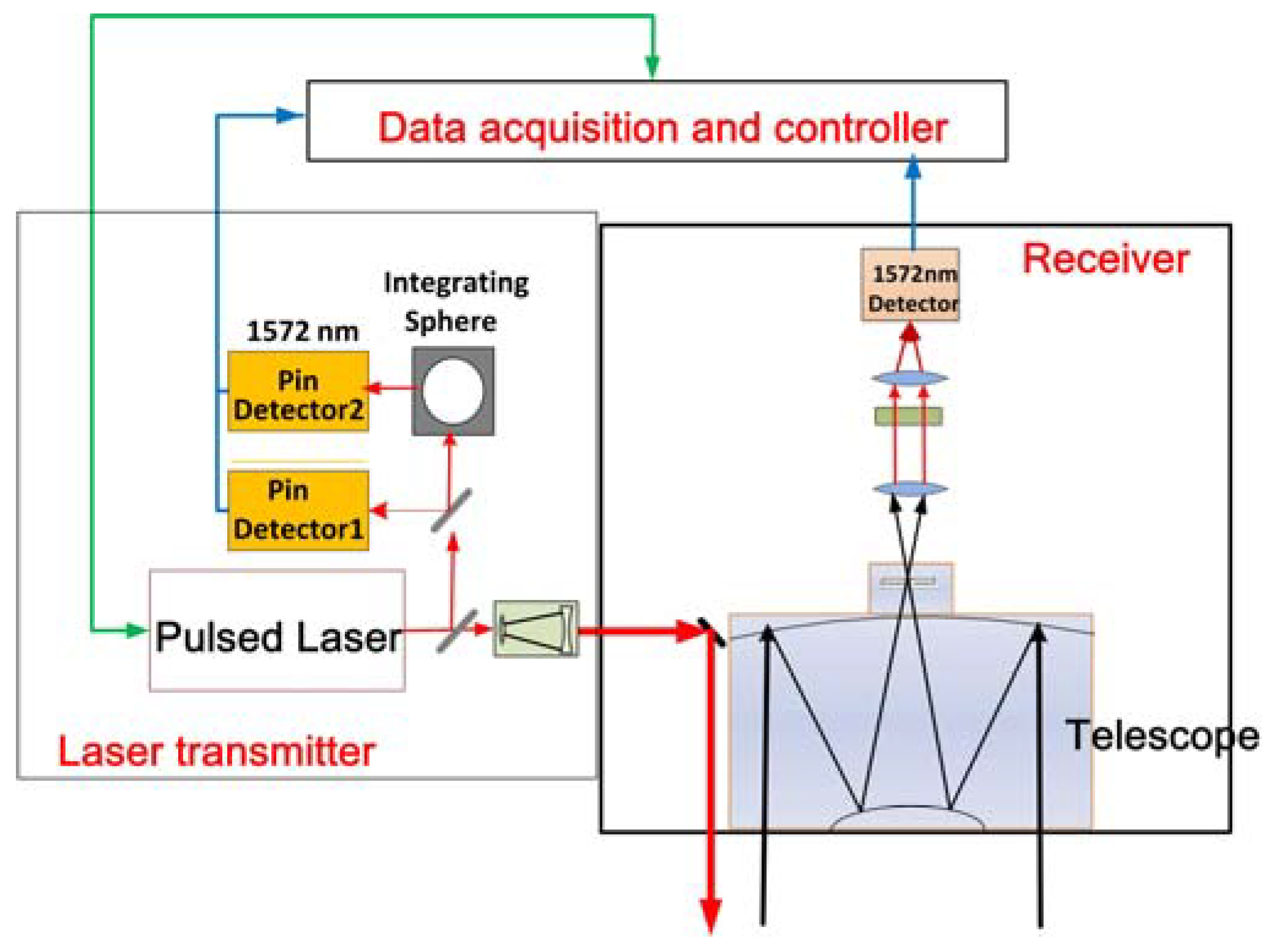
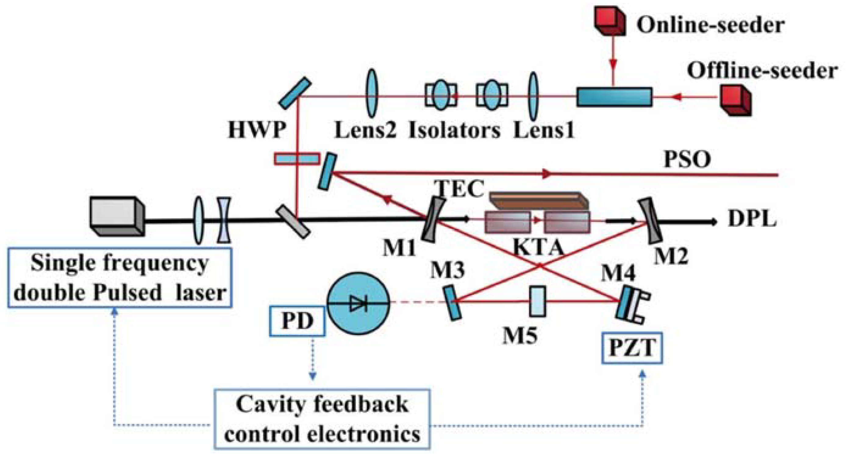
2.1. Introduction to the Instrumentation
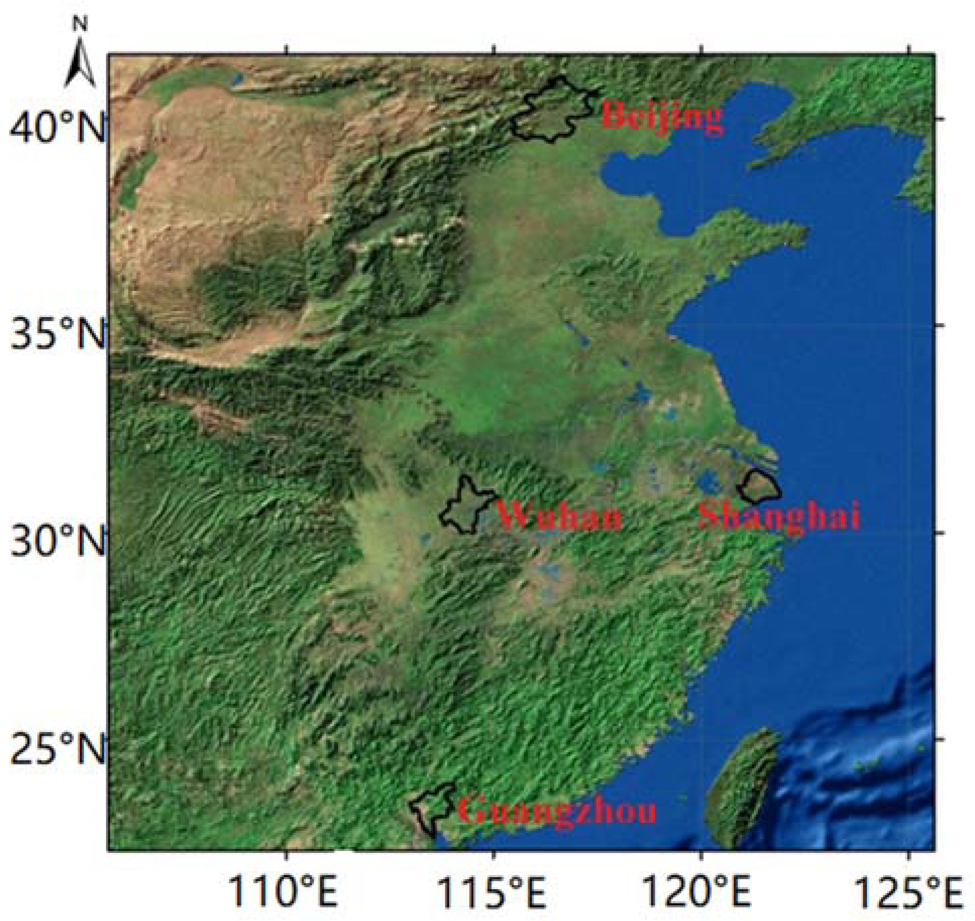
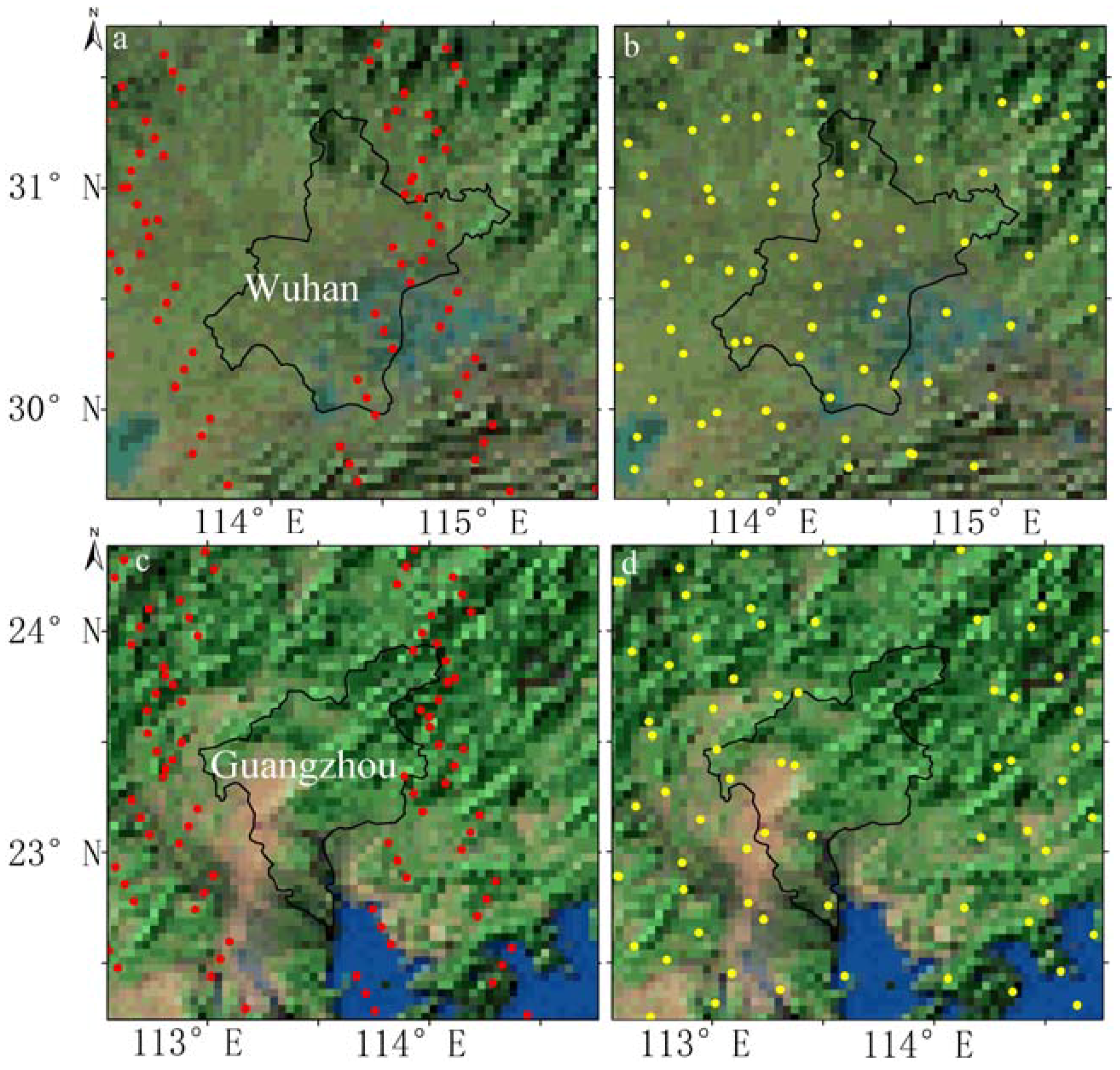
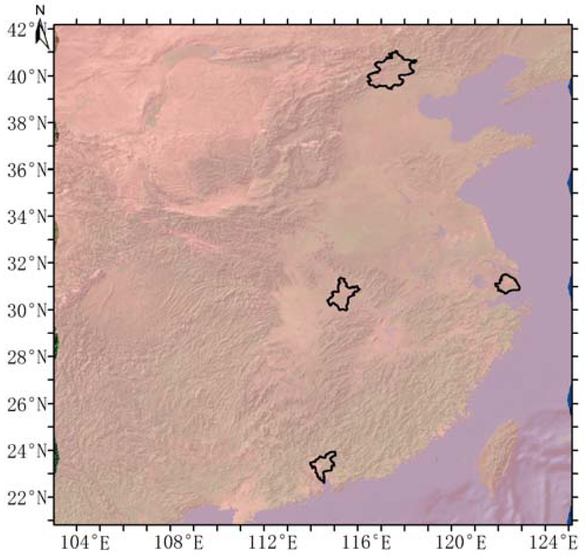
2.2. Study Area
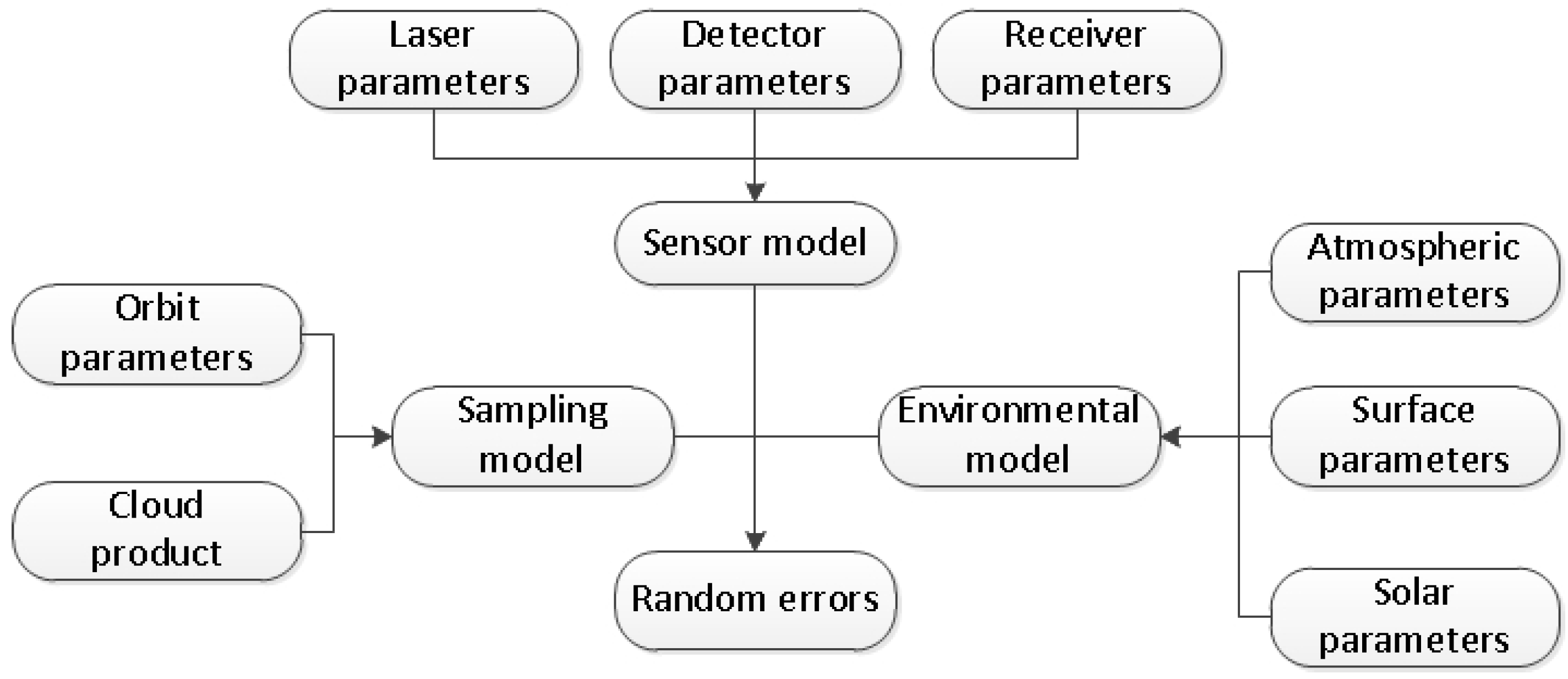
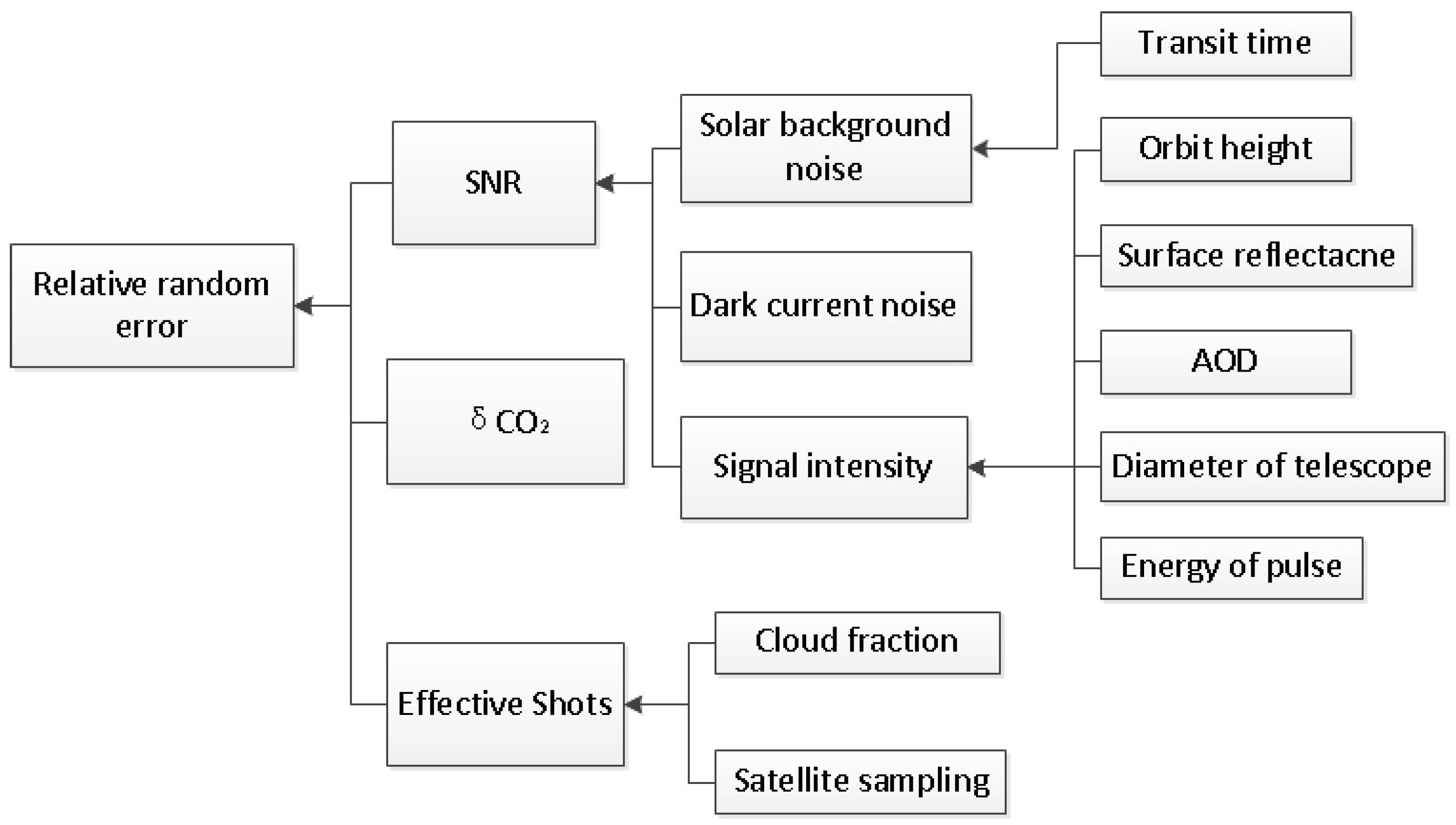
2.3. Random Errors
2.4. Systematic Errors
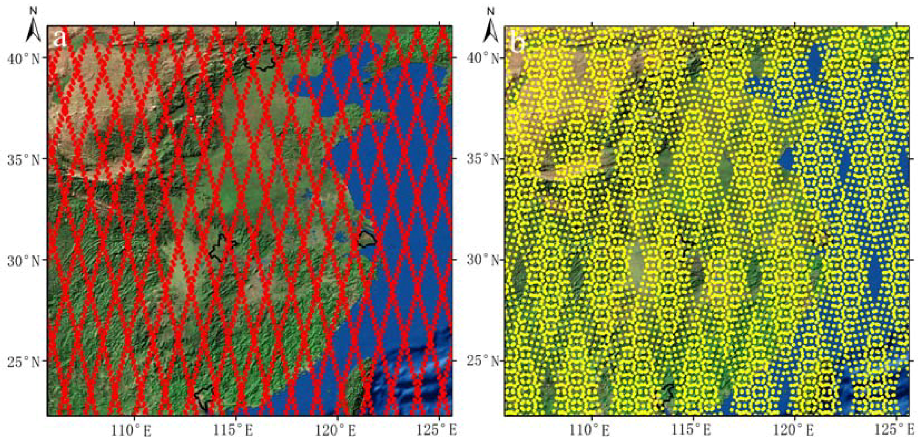
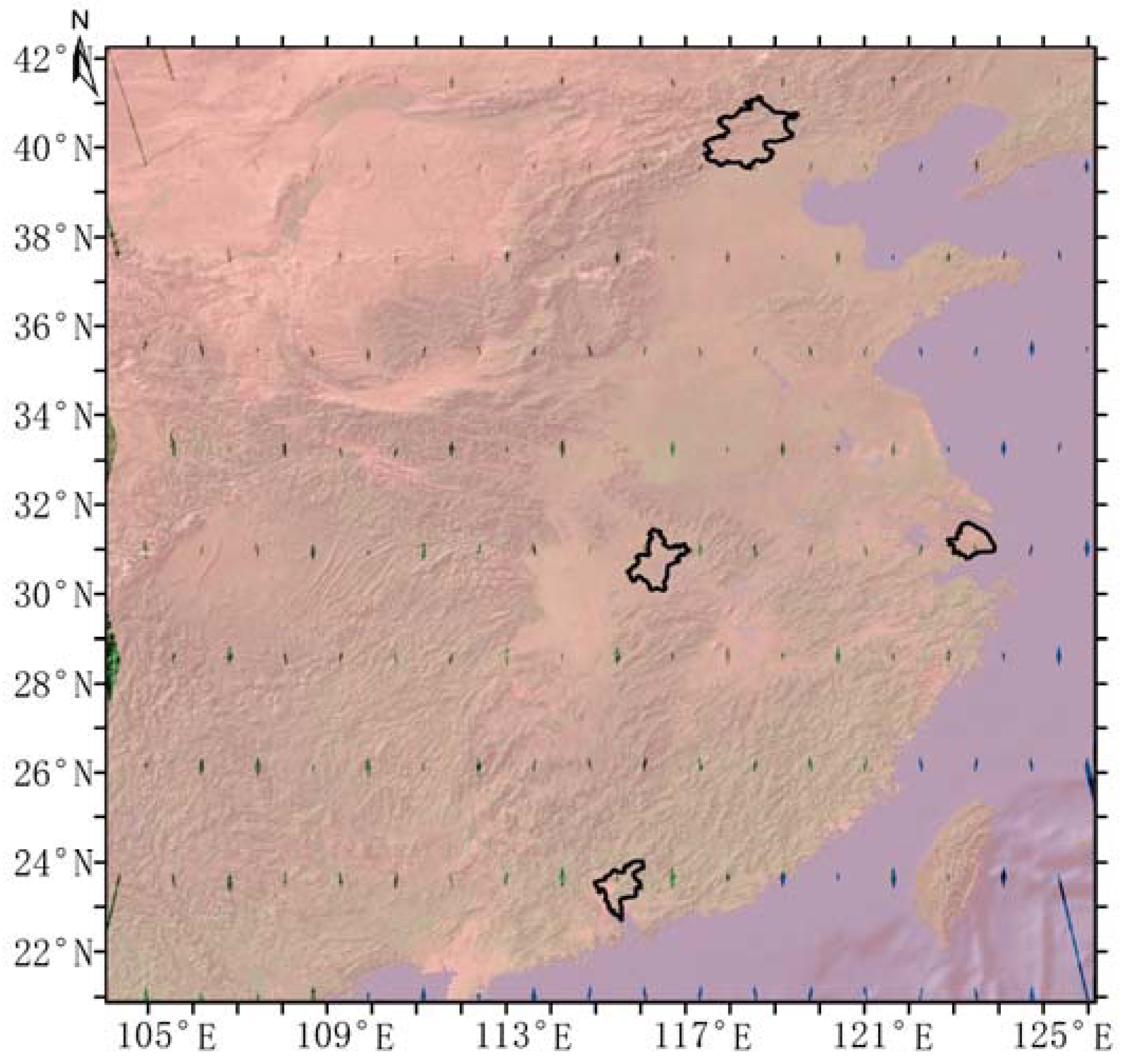
2.5. Orbit Sampling
2.6. Study Materials
3. Results
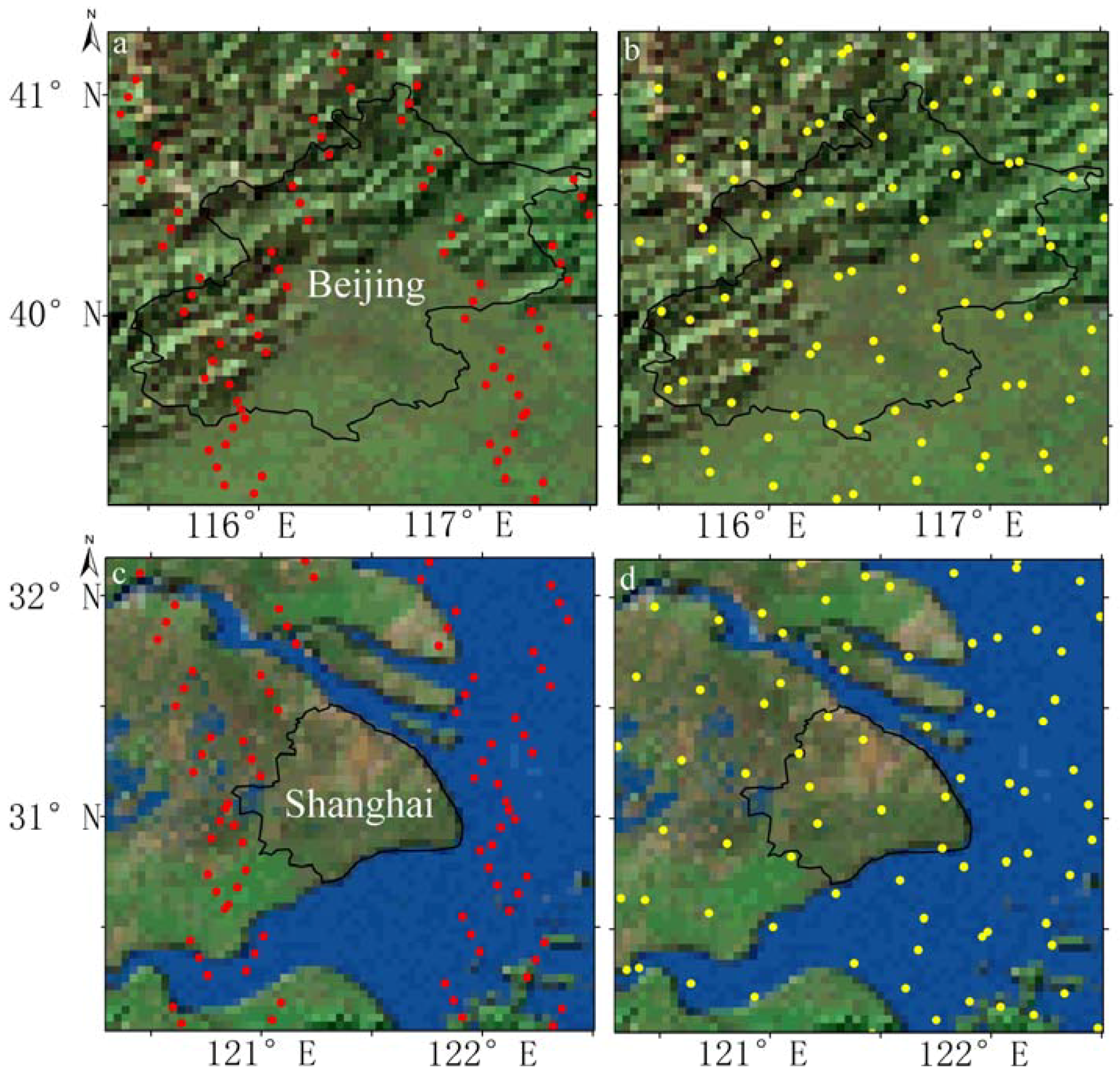
3.1. Sample Point Distributions
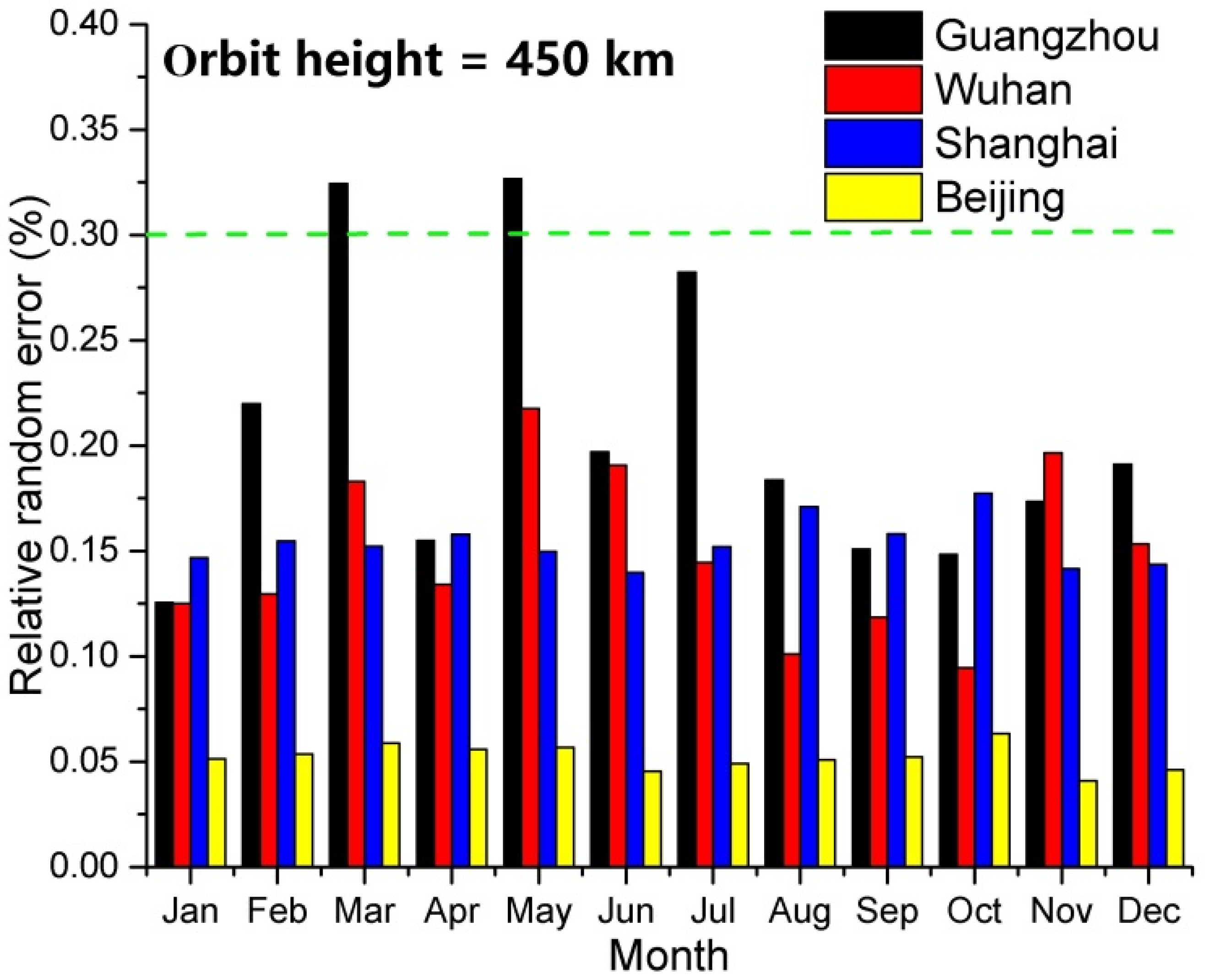
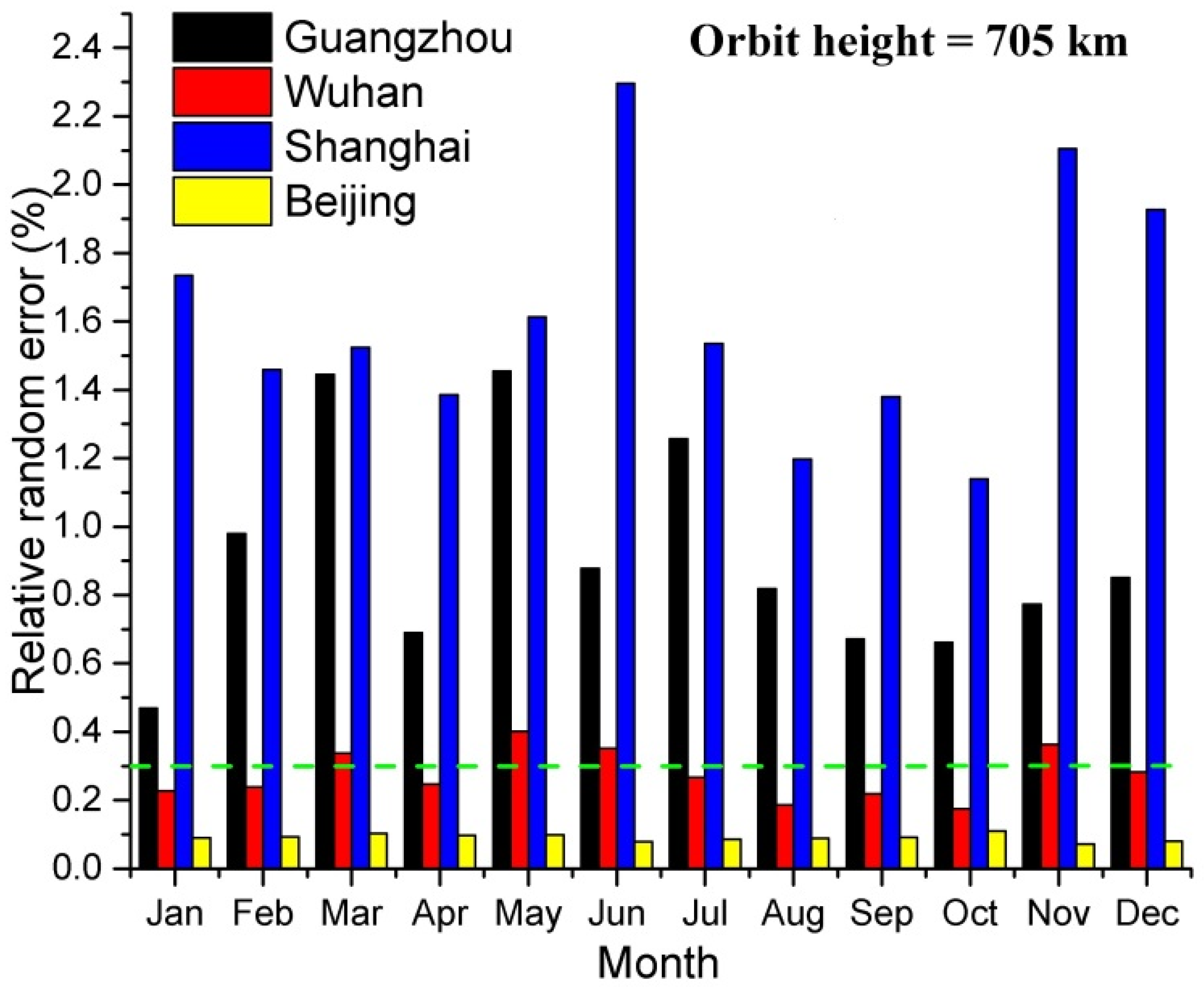
3.2. Estimation of the Random Error
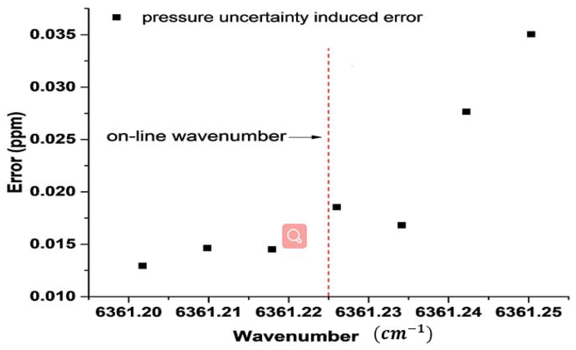
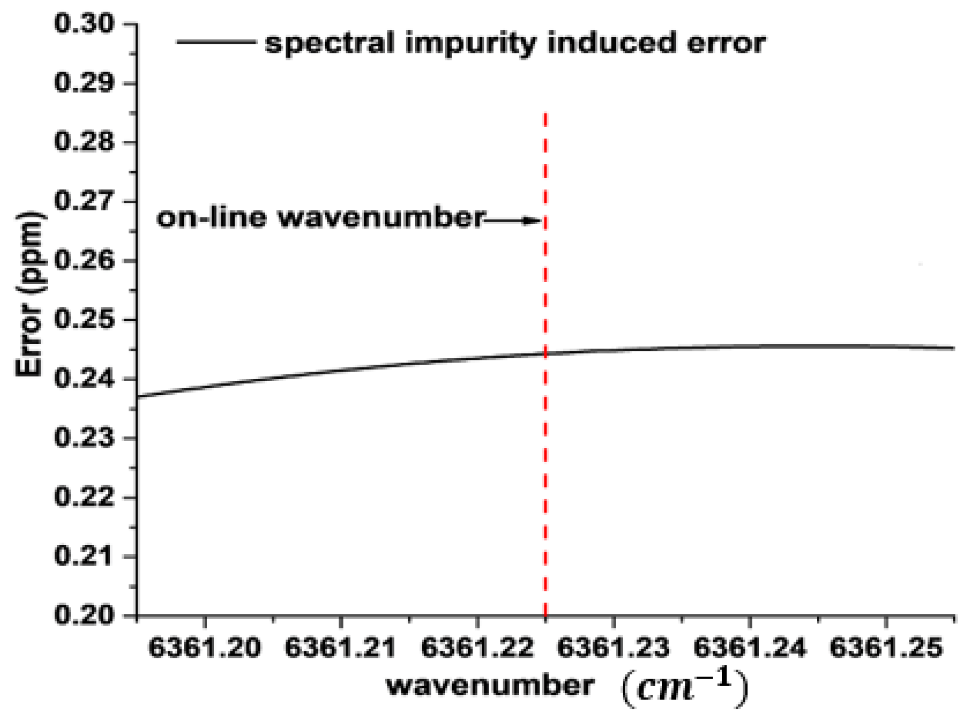
3.3. Estimation of the Systematic Error
4. Discussion
4.1. Potential Uncertainty Due to the AOD Products
4.2. Potential of Off-Nadir Modes
4.3. Potential Scientific Applications
4.4. Further Demands for Improvements of Systematic Errors
5. Conclusions
Author Contributions
Funding
Acknowledgments
Conflicts of Interest
Appendix A. Introduction to ASEM-CO2-IPDA

| Category | Parameter Name | Value | Unit |
|---|---|---|---|
| Laser transmitter | Pulse length | 15 | ns |
| On-line wavelength | 6361.225 | cm−1 | |
| Off-line wavelength | 6360.981 | cm−1 | |
| Fluctuation of pulse energy | 1 | % | |
| Fluctuation of ratio of on-line and off-line pulse energy | 0.1 | % | |
| Linewidth | 50 | MHz | |
| Stability of on-line wavelength | 0.6 | MHz | |
| Spectral purity | 99.9 | % | |
| Energy per pulse | 75 | mJ | |
| Repetition frequency (a pair of on-line and off-line) | 20 | Hz | |
| Interval time between successive beams | 200 | us | |
| Divergence angle | 100 | urad | |
| Telescope | Time interval of contiguous pair | 0.2 | ms |
| Diameter | 1 | m | |
| Overall optical efficiency | 51.8 | % | |
| Optical filter bandwidth | 0.45 | nm | |
| Field of view | 0.2 | mrad | |
| Electronic bandwidth | 3 | MHz | |
| Dark current (noise equivalent power) | 64 | fW/ | |
| Quantum efficiency | 73 | % | |
| Internal gain | 9 | ||
| Excess noise factor | 3.2 | ||
| Other | Orbit altitude | 705 | km |
| Orbit type | 1 h/13 h sun-synchronous | ||
| Viewing geometry | Nadir |


Appendix B. Description of Calculation Method of the Random Error

References
- Stocker, T.F.; Qin, D.; Plattner, G.-K.; Tignor, M.; Allen, S.K.; Boschung, J.; Nauels, A.; Xia, Y.; Bex, V.; Midgley, P.M. IPCC, 2013: Climate change 2013: The physical science basis. In Contribution of Working Group I to the Fifth Assessment Report of the Intergovernmental Panel on Climate Change; Cambridge University Press: Cambridge, UK; New York, NY, USA, 2013. [Google Scholar]
- Liu, L.; Chen, C.; Zhao, Y.; Zhao, E. China’s carbon-emissions trading: Overview, challenges and future. Renew. Sustain. Energy Rev. 2015, 49, 254–266. [Google Scholar] [CrossRef]
- Birol, F. World Energy Outlook 2010; International Energy Agency: Paris, France, 2010. [Google Scholar]
- Sellers, P.; Dickinson, R.; Randall, D.; Betts, A.; Hall, F.; Berry, J.; Collatz, G.; Denning, A.; Mooney, H.; Nobre, C. Modeling the exchanges of energy, water, and carbon between continents and the atmosphere. Science 1997, 275, 502–509. [Google Scholar] [CrossRef] [PubMed]
- Normile, D. Round and round a guide to the carbon cycle. Science 2009, 325, 1642–1643. [Google Scholar] [CrossRef] [PubMed]
- Gurney, K.R.; Law, R.M.; Denning, A.S.; Rayner, P.J.; Baker, D.; Bousquet, P.; Bruhwiler, L.; Chen, Y.H.; Ciais, P.; Fan, S.; et al. Towards robust regional estimates of CO2 sources and sinks using atmospheric transport models. Nature 2002, 415, 626–630. [Google Scholar] [CrossRef] [PubMed]
- Rayner, P.; O’Brien, D. The utility of remotely sensed CO2 concentration data in surface source inversions. Geophys. Res. Lett. 2001, 28, 175–178. [Google Scholar] [CrossRef]
- Paris, J.D.; Ciais, P.; Nédélec, P.; Ramonet, M.; Belan, B.; Arshinov, M.; Golitsyn, G.; Granberg, I.; Stohl, A.; Cayez, G. The YAK-AEROSIB transcontinental aircraft campaigns: New insights on the transport of CO2, CO and O3 across siberia. Tellus B 2008, 60, 551–568. [Google Scholar] [CrossRef]
- Lin, J.; Gerbig, C.; Wofsy, S.; Daube, B.; Matross, D.; Chow, V.; Gottlieb, E.; Andrews, A.; Pathmathevan, M.; Munger, J. What have we learned from intensive atmospheric sampling field programmes of CO2? Tellus B 2006, 58, 331–343. [Google Scholar] [CrossRef]
- LAI, C.T.; Schauer, A.J.; Owensby, C.; Ham, J.M.; Helliker, B.; Tans, P.P.; Ehleringer, J.R. Regional CO2 fluxes inferred from mixing ratio measurements: Estimates from flask air samples in central Kansas, USA. Tellus B 2006, 58, 523–536. [Google Scholar] [CrossRef]
- McKain, K.; Wofsy, S.C.; Nehrkorn, T.; Eluszkiewicz, J.; Ehleringer, J.R.; Stephens, B.B. Assessment of ground-based atmospheric observations for verification of greenhouse gas emissions from an urban region. Proc. Natl. Acad. Sci. USA 2012, 109, 8423–8428. [Google Scholar] [CrossRef] [PubMed]
- Chevallier, F.; Maksyutov, S.; Bousquet, P.; Bréon, F.M.; Saito, R.; Yoshida, Y.; Yokota, T. On the accuracy of the CO2 surface fluxes to be estimated from the gosat observations. Geophys. Res. Lett. 2009, 36. [Google Scholar] [CrossRef]
- Liu, Y.; Yang, D.; Cai, Z. A retrieval algorithm for tansat XCO2 observation: Retrieval experiments using gosat data. Chin. Sci. Bull. 2013, 58, 1520–1523. [Google Scholar] [CrossRef]
- Miller, J.B.; Tans, P.P.; Gloor, M. Steps for success of OCO-2. Nat. Geosci. 2014, 7, 691. [Google Scholar] [CrossRef]
- Crisp, D.; Bösch, H.; Brown, L.; Castano, R.; Christi, M.; Connor, B.; Frankenberg, C.; McDuffie, J.; Miller, C.; Natraj, V. OCO (Orbiting Carbon Observatory)-2 Level 2 Full Physics Retrieval Algorithm Theoretical Basis. 2010. Available online: http://disc.sci.gsfc.nasa.gov/acdisc/documentation/OCO-2_L2_FP_ATBDv1_rev4_Nov10.pdf (accessed on 19 June 2018).
- Connor, B.; Bosch, H.; McDuffie, J.; Taylor, T.; Fu, D.J.; Frankenberg, C.; O’Dell, C.; Payne, V.H.; Gunson, M.; Pollock, R.; et al. Quantification of uncertainties in OCO-2 measurements of XCO2: Simulations and linear error analysis. Atmos. Meas. Tech. 2016, 9, 5227–5238. [Google Scholar] [CrossRef]
- Houweling, S.; Hartmann, W.; Aben, I.; Schrijver, H.; Skidmore, J.; Roelofs, G.-J.; Breon, F.-M. Evidence of systematic errors in sciamachy-observed CO2 due to aerosols. Atmos. Chem. Phys. 2005, 5, 3003–3013. [Google Scholar] [CrossRef]
- Liang, A.; Han, G.; Gong, W.; Yang, J.; Xiang, C. Comparison of global XCO2 concentrations from OCO-2 with tccon data in terms of latitude zones. IEEE J. Sel. Top. Appl. Earth Obs. Remote Sens. 2017, 10, 2491–2498. [Google Scholar] [CrossRef]
- Liang, A.L.; Gong, W.; Han, G.; Xiang, C.Z. Comparison of satellite-observed XCO2 from gosat, OCO-2, and ground-based tccon. Remote Sens. 2017, 9, 1033. [Google Scholar] [CrossRef]
- Menzies, R.T.; Tratt, D.M. Differential laser absorption spectrometry for global profiling of tropospheric carbon dioxide: Selection of optimum sounding frequencies for high-precision measurements. Appl. Opt. 2003, 42, 6569–6577. [Google Scholar] [CrossRef] [PubMed]
- Han, G.; Cui, X.; Liang, A.; Ma, X.; Zhang, T.; Gong, W. A CO2 profile retrieving method based on chebyshev fitting for ground-based dial. IEEE Trans. Geosci. Remote Sens. 2017, 55, 6099–6110. [Google Scholar] [CrossRef]
- Abshire, J.B.; Ramanathan, A.; Riris, H.; Mao, J.P.; Allan, G.R.; Hasselbrack, W.E.; Weaver, C.J.; Browell, E.V. Airborne measurements of CO2 column concentration and range using a pulsed direct- detection ipda LIDAR. Remote Sens. 2014, 6, 443–469. [Google Scholar] [CrossRef]
- Lin, B.; Nehrir, A.R.; Harrison, F.W.; Browell, E.V.; Ismail, S.; Obland, M.D.; Campbell, J.; Dobler, J.; Meadows, B.; Fan, T.-F.; et al. Atmospheric CO2 column measurements in cloudy conditions using intensity-modulated continuous-wave LIDAR at 1.57 micron. Opt. Express 2015, 23, A582–A593. [Google Scholar] [CrossRef] [PubMed]
- Refaat, T.F.; Singh, U.N.; Yu, J.; Petros, M.; Ismail, S.; Kavaya, M.J.; Davis, K.J. Evaluation of an airborne triple-pulsed 2 μm ipda LIDAR for simultaneous and independent atmospheric water vapor and carbon dioxide measurements. Appl. Opt. 2015, 54, 1387–1398. [Google Scholar] [CrossRef] [PubMed]
- Yu, J.; Petros, M.; Singh, U.N.; Refaat, T.F.; Reithmaier, K.; Remus, R.G.; Johnson, W. An airborne 2-μm double-pulsed direct-detection LIDAR instrument for atmospheric CO2 column measurements. J. Atmos. Ocean. Technol. 2017, 34, 385–400. [Google Scholar] [CrossRef]
- Amediek, A.; Ehret, G.; Fix, A.; Wirth, M.; Budenbender, C.; Quatrevalet, M.; Kiemle, C.; Gerbig, C. CHARM-F—A new airborne integrated-path differential-absorption LIDAR for carbon dioxide and methane observations: Measurement performance and quantification of strong point source emissions. Appl. Opt. 2017, 56, 5182–5197. [Google Scholar] [CrossRef] [PubMed]
- Amediek, A.; Fix, A.; Wirth, M.; Ehret, G. Development of an opo system at 1.57 μm for integrated path dial measurement of atmospheric carbon dioxide. Appl. Phys. B 2008, 92, 295–302. [Google Scholar] [CrossRef]
- Amediek, A.; Sun, X.L.; Abshire, J.B. Analysis of range measurements from a pulsed airborne CO2 integrated path differential absorption LIDAR. IEEE Trans. Geosci. Remote Sens. 2013, 51, 2498–2504. [Google Scholar] [CrossRef]
- Dobler, J.; Braun, M.; Blume, N.; Zaccheo, T.S. A new laser based approach for measuring atmospheric greenhouse gases. Remote Sens. 2013, 5, 6284–6304. [Google Scholar] [CrossRef]
- Menzies, R.T.; Spiers, G.D.; Jacob, J. Airborne laser absorption spectrometer measurements of atmospheric CO2 column mole fractions: Source and sink detection and environmental impacts on retrievals. J. Atmos. Ocean. Technol. 2014, 31, 404–421. [Google Scholar] [CrossRef]
- Kameyama, S.; Imaki, M.; Hirano, Y.; Ueno, S.; Kawakami, S.; Sakaizawa, D.; Kimura, T.; Nakajima, M. Feasibility study on 1.6 μm continuous-wave modulation laser absorption spectrometer system for measurement of global CO2 concentration from a satellite. Appl. Opt. 2011, 50, 2055–2068. [Google Scholar] [CrossRef] [PubMed]
- Sakaizawa, D.; Kawakami, S.; Nakajima, M.; Sawa, Y.; Matsueda, H.; Asai, K.; Kameyama, S.; Imaki, M.; Hirano, Y.; Ueno, S. Path-averaged atmospheric CO2 measurement using a 1.57 μm active remote sensor compared with multi-positioned in situ sensors. Proc. SPIE 2009. [Google Scholar] [CrossRef]
- Han, G.; Ma, X.; Liang, A.; Zhang, T.; Zhao, Y.; Zhang, M.; Gong, W. Performance evaluation for China’s planned CO2-ipda. Remote Sens. 2017, 9, 768. [Google Scholar] [CrossRef]
- Ingmann, P.; Bensi, P.; Durand, Y. A-scope-advanced space carbon and climate observation of planet erath. In ESA Report for Assessment, SP-1313/1; ESA Communication Production Office: Noordwijk, The Netherlands, 2008. [Google Scholar]
- Hakkarainen, J.; Ialongo, I.; Tamminen, J. Direct space-based observations of anthropogenic CO2 emission areas from OCO-2. Geophys. Res. Lett. 2016, 43. [Google Scholar] [CrossRef]
- Kiemle, C.; Ehret, G.; Amediek, A.; Fix, A.; Quatrevalet, M.; Wirth, M. Potential of spaceborne LIDAR measurements of carbon dioxide and methane emissions from strong point sources. Remote Sens. 2017, 9, 1137. [Google Scholar] [CrossRef]
- Bousquet, P.; Peylin, P.; Ciais, P.; Ramonet, M.; Monfray, P. Inverse modeling of annual atmospheric CO2 sources and sinks: 2. Sensitivity study. J. Geophys. Res. Atmos. 1999, 104, 26179–26193. [Google Scholar] [CrossRef]
- Bousquet, P.; Ciais, P.; Peylin, P.; Ramonet, M.; Monfray, P. Inverse modeling of annual atmospheric CO2 sources and sinks: 1. Method and control inversion. J. Geophys. Res. Atmos. 1999, 104, 26161–26178. [Google Scholar] [CrossRef]
- Ehret, G.; Kiemle, C.; Wirth, M.; Amediek, A.; Fix, A.; Houweling, S. Space-borne remote sensing of CO2, CH4, and N2O by integrated path differential absorption LIDAR: A sensitivity analysis. Appl. Phys. B 2008, 90, 593–608. [Google Scholar] [CrossRef]
- Kawa, S.; Mao, J.; Abshire, J.; Collatz, G.; Sun, X.; Weaver, C. Simulation studies for a space-based CO2 LIDAR mission. Tellus B 2010, 62, 759–769. [Google Scholar] [CrossRef]
- Kiemle, C.; Kawa, S.R.; Quatrevalet, M.; Browell, E.V. Performance simulations for a spaceborne methane LIDAR mission. J. Geophys. Res. Atmos. 2014, 119, 4365–4379. [Google Scholar] [CrossRef]
- Mao, J.; Ramanathan, A.; Abshire, J.B.; Kawa, S.R.; Riris, H.; Allan, G.R.; Rodriguez, M.; Hasselbrack, W.E.; Sun, X.; Numata, K. Measurement of atmospheric CO2 column concentrations to cloud tops with a pulsed multi-wavelength airborne LIDAR. Atmos. Meas. Tech. 2018, 11, 1–26. [Google Scholar] [CrossRef]
- Ramanathan, A.K.; Mao, J.P.; Abshire, J.B.; Allan, G.R. Remote sensing measurements of the CO2 mixing ratio in the planetary boundary layer using cloud slicing with airborne LIDAR. Geophys. Res. Lett. 2015, 42, 2055–2062. [Google Scholar] [CrossRef]
- Kiemle, C.; Quatrevalet, M.; Ehret, G.; Amediek, A.; Fix, A.; Wirth, M. Sensitivity studies for a space-based methane LIDAR mission. Atmos. Meas. Tech. 2011, 4, 2195–2211. [Google Scholar] [CrossRef]
- Predoi-Cross, A.; McKella, A.R.W.; Chiris Benner, D.; Devi, M.V.; Gamache, R.R.; Miller, C.E.; Toth, R.A.; Brown, L.R. Temperature dependences for air-broadened lorentz half-width and pressure shift coefficients in the 30013←00001 and 30012←00001 bands of CO2 near 1600 nm. Can. J. Phys. 2009, 87, 517–535. [Google Scholar] [CrossRef]
- Rothman, L.S.; Gordon, I.E.; Babikov, Y.; Barbe, A.; Chris Benner, D.; Bernath, P.F.; Birk, M.; Bizzocchi, L.; Boudon, V.; Brown, L.R.; et al. The hitran2012 molecular spectroscopic database. J. Quant. Spectrosc. Radiat. Transf. 2013, 130, 4–50. [Google Scholar] [CrossRef]
- Du, J.; Zhu, Y.D.; Li, S.G.; Zhang, J.X.; Sun, Y.G.; Zang, H.G.; Liu, D.; Ma, X.H.; Bi, D.C.; Liu, J.Q.; et al. Double-pulse 1.57 mu m integrated path differential absorption LIDAR ground validation for atmospheric carbon dioxide measurement. Appl. Opt. 2017, 56, 7053–7058. [Google Scholar] [CrossRef] [PubMed]
- Singh, U.N.; Refaat, T.F.; Ismail, S.; Davis, K.J.; Kawa, S.R.; Menzies, R.T.; Petros, M. Feasibility study of a space-based high pulse energy 2 μm CO2 ipda LIDAR. Appl. Opt. 2017, 56, 6531–6547. [Google Scholar] [CrossRef] [PubMed]
- Amediek, A.; Fix, A.; Ehret, G.; Caron, J.; Durand, Y. Airborne LIDAR reflectance measurements at 1.57 mu m in support of the a-scope mission for atmospheric CO2. Atmos. Meas. Tech. 2009, 2, 755–772. [Google Scholar] [CrossRef]
- Disney, M.I.; Lewis, P.E.; Bouvet, M.; Prieto-Blanco, A.; Hancock, S. Quantifying surface reflectivity for spaceborne LIDAR via two independent methods. IEEE Trans. Geosci. Remote Sens. 2009, 47, 3262–3271. [Google Scholar] [CrossRef]
- Han, G.; Gong, W.; Quan, J.; Li, J.; Zhang, M. Study on spatial and temporal distributions of contaminants emitted by chinese new year’eve celebrations in wuhan. Environ. Sci. Process. Impacts 2014, 16, 916–923. [Google Scholar] [CrossRef] [PubMed]
- Hutchison, K.D.; Smith, S.; Faruqui, S. The use of MODIS data and aerosol products for air quality prediction. Atmos. Environ. 2004, 38, 5057–5070. [Google Scholar] [CrossRef]
- Gupta, P.; Christopher, S.A.; Wang, J.; Gehrig, R.; Lee, Y.; Kumar, N. Satellite remote sensing of particulate matter and air quality assessment over global cities. Atmos. Environ. 2006, 40, 5880–5892. [Google Scholar] [CrossRef]
- Cyranoski, D. Satellite view alerts china to soaring pollution. Nature 2005, 437, 12. [Google Scholar] [CrossRef] [PubMed]
- Bovensmann, H.; Buchwitz, M.; Burrows, J.P.; Reuter, M.; Krings, T.; Gerilowski, K.; Schneising, O.; Heymann, J.; Tretner, A.; Erzinger, J. A remote sensing technique for global monitoring of power plant CO2 emissions from space and related applications. Atmos. Meas. Tech. 2010, 3, 781–811. [Google Scholar] [CrossRef]
- Kotthaus, S.; Grimmond, C.S.B. Identification of micro-scale anthropogenic CO2, heat and moisture sources—processing eddy covariance fluxes for a dense urban environment. Atmos. Environ. 2012, 57, 301–316. [Google Scholar] [CrossRef]
- Aiuppa, A.; Fiorani, L.; Santoro, S.; Parracino, S.; Nuvoli, M.; Chiodini, G.; Minopoli, C.; Tamburello, G. New ground-based LIDAR enables volcanic CO2 flux measurements. Sci. Rep. 2015, 5, 13614. [Google Scholar] [CrossRef] [PubMed]
- Han, G.; Gong, W.; Lin, H.; Ma, X.; Xiang, Z. Study on influences of atmospheric factors on vertical profile retrieving from ground-based dial at 1.6 μm. IEEE Trans. Geosci. Remote Sens. 2015, 53, 3221–3234. [Google Scholar] [CrossRef]
- Han, G.; Gong, W.; Lin, H.; Ma, X.; Xiang, C. On-line wavelength calibration of pulsed laser for CO2 dial sensing. Appl. Phys. B 2014, 117, 1041–1053. [Google Scholar] [CrossRef]
- Koch, G.J.; Beyon, J.Y.; Gibert, F.; Barnes, B.W.; Ismail, S.; Petros, M.; Petzar, P.J.; Yu, J.; Modlin, E.A.; Davis, K.J. Side-line tunable laser transmitter for differential absorption LIDAR measurements of CO2: Design and application to atmospheric measurements. Appl. Opt. 2008, 47, 944–956. [Google Scholar] [CrossRef] [PubMed]
- Nichol, J.; Bilal, M. Validation of MODIS 3 km resolution aerosol optical depth retrievals over asia. Remote Sens. 2016, 8, 328. [Google Scholar] [CrossRef]
- He, Q.; Li, C.; Tang, X.; Li, H.; Geng, F.; Wu, Y. Validation of MODIS derived aerosol optical depth over the yangtze river delta in china. Remote Sens. Environ. 2012, 114, 1649–1661. [Google Scholar] [CrossRef]
- Man, S.W.; Shahzad, M.; Nichol, J.; Chan, P.W.; Chan, P.W. Validation of MODIS, misr, omi, and calipso aerosol optical thickness using ground-based sunphotometers in Hong Kong. Int. J. Remote Sens. 2013, 34, 897–918. [Google Scholar]
- Wang, W.; Mao, F.; Pan, Z.; Du, L.; Gong, W. Validation of viirs aod through a comparison with a sun photometer and MODIS aods over Wuhan. Remote Sens. 2017, 9, 403. [Google Scholar] [CrossRef]
- Han, G.; Gong, W.; Ma, X.; Xiang, C.; Liang, A.; Zheng, Y. A ground-based differential absorption LIDAR for atmospheric vertical CO2 profiling. Acta Phys. Sin. 2015, 64, 244206. [Google Scholar]
- Hill, C.; Gordon, I.E.; Kochanov, R.V.; Barrett, L.; Wilzewski, J.S.; Rothman, L.S. Hitranonline: An online interface and the flexible representation of spectroscopic data in the hitran database. J. Quant. Spectrosc. Radiat. Transf. 2016, 177, 4–14. [Google Scholar] [CrossRef]
- Han, G.; Xu, H.; Gong, W.; Ma, X.; Liang, A. Simulations of a multi-wavelength differential absorption LIDAR method for CO2 measurement. Appl. Opt. 2017, 56, 8532–8540. [Google Scholar] [CrossRef] [PubMed]
- Caron, J.; Durand, Y. Operating wavelengths optimization for a spaceborne LIDAR measuring atmospheric CO2. Appl. Opt. 2009, 48, 5413–5422. [Google Scholar] [CrossRef] [PubMed]


| Category | Name | Uncertainty |
|---|---|---|
| Atmospheric effect | Temperature | 0.5 K |
| Pressure | 0.5 hPa | |
| Humidity | 10% | |
| Line parameter | Line strength | 2% |
| Pressure shift | 1% | |
| Pressure broadening | 0.08% | |
| Temperature scaling exponent | 0.72% | |
| Laser | Frequency drift | 0.6 MHz |
| spectral purity | 99.9% + 0.45 nm | |
| Satellite | Doppler shift along track | 140 µrad |
| Doppler shift across track | 1000 µrad | |
| Misalignment of footprint | 25 µrad | |
| Ranging accuracy | 2 m |
| Abbr. | Description/Value | Unit |
|---|---|---|
| δ | The latitude | degree |
| α | The longitude | degree |
| n | The angular velocity of satellite | rad/s |
| t | Any given time | s |
| t0 | The time at which the satellite passes the ascending node | s |
| Δα | The differential longitude between the ascending node and the current nadir | degree |
| ω | The angular velocity of earth/7.29 × 10−5 | rad/s |
| i | The orbit inclination/98.2 | degree |
| μ | The geocentric gravitational constant/3.986 × 1014 | m3/s2 |
| a | The semi-major axis of satellite orbit | km |
| Hsatellite | The altitude of satellite/705 or 450 in this work | km |
| Tsatellite | The orbit period | s |
| Name | Guangzhou | Wuhan | Shanghai | Beijing | |
|---|---|---|---|---|---|
| Annual AOD | 0.64 | 0.78 | 0.95 | 0.54 | |
| annual reflectance | 0.168 | 0.170 | 0.156 | 0.190 | |
| Area (km2) | 7343 | 8594 | 6340 | 1,6410 | |
| Number of observations in 1 month | 450 km | 838 | 1625 | 745 | 3631 |
| 705 km | 142 | 1232 | 56 | 2626 | |
| Monthly cloud fraction (%) | Jan. | 48.74 | 66.96 | 80.73 | 55.17 |
| Feb. | 83.32 | 69.21 | 72.74 | 50.75 | |
| Mar. | 92.33 | 84.55 | 75.02 | 42.04 | |
| Apr. | 66.36 | 71.18 | 69.78 | 46.77 | |
| May | 92.44 | 89.08 | 77.72 | 45.32 | |
| Jun. | 79.23 | 85.77 | 89.00 | 70.77 | |
| Jul. | 89.88 | 75.20 | 75.38 | 60.47 | |
| Aug. | 76.10 | 49.3 | 59.52 | 56.10 | |
| Sep. | 64.50 | 63.21 | 69.54 | 53.55 | |
| Oct. | 63.38 | 42.06 | 55.26 | 36.33 | |
| Nov. | 73.20 | 86.60 | 86.90 | 87.33 | |
| Dec. | 77.92 | 78.00 | 84.37 | 68.23 | |
© 2018 by the authors. Licensee MDPI, Basel, Switzerland. This article is an open access article distributed under the terms and conditions of the Creative Commons Attribution (CC BY) license (http://creativecommons.org/licenses/by/4.0/).
Share and Cite
Han, G.; Xu, H.; Gong, W.; Liu, J.; Du, J.; Ma, X.; Liang, A. Feasibility Study on Measuring Atmospheric CO2 in Urban Areas Using Spaceborne CO2-IPDA LIDAR. Remote Sens. 2018, 10, 985. https://doi.org/10.3390/rs10070985
Han G, Xu H, Gong W, Liu J, Du J, Ma X, Liang A. Feasibility Study on Measuring Atmospheric CO2 in Urban Areas Using Spaceborne CO2-IPDA LIDAR. Remote Sensing. 2018; 10(7):985. https://doi.org/10.3390/rs10070985
Chicago/Turabian StyleHan, Ge, Hao Xu, Wei Gong, Jiqiao Liu, Juan Du, Xin Ma, and Ailin Liang. 2018. "Feasibility Study on Measuring Atmospheric CO2 in Urban Areas Using Spaceborne CO2-IPDA LIDAR" Remote Sensing 10, no. 7: 985. https://doi.org/10.3390/rs10070985
APA StyleHan, G., Xu, H., Gong, W., Liu, J., Du, J., Ma, X., & Liang, A. (2018). Feasibility Study on Measuring Atmospheric CO2 in Urban Areas Using Spaceborne CO2-IPDA LIDAR. Remote Sensing, 10(7), 985. https://doi.org/10.3390/rs10070985