Antarctic Surface Ice Velocity Retrieval from MODIS-Based Mosaic of Antarctica (MOA)


Abstract
1. Introduction
2. Data
2.1. MOA
2.2. Landsat-8 Rock Outcrop
2.3. MEaSUREs Ice Velocity
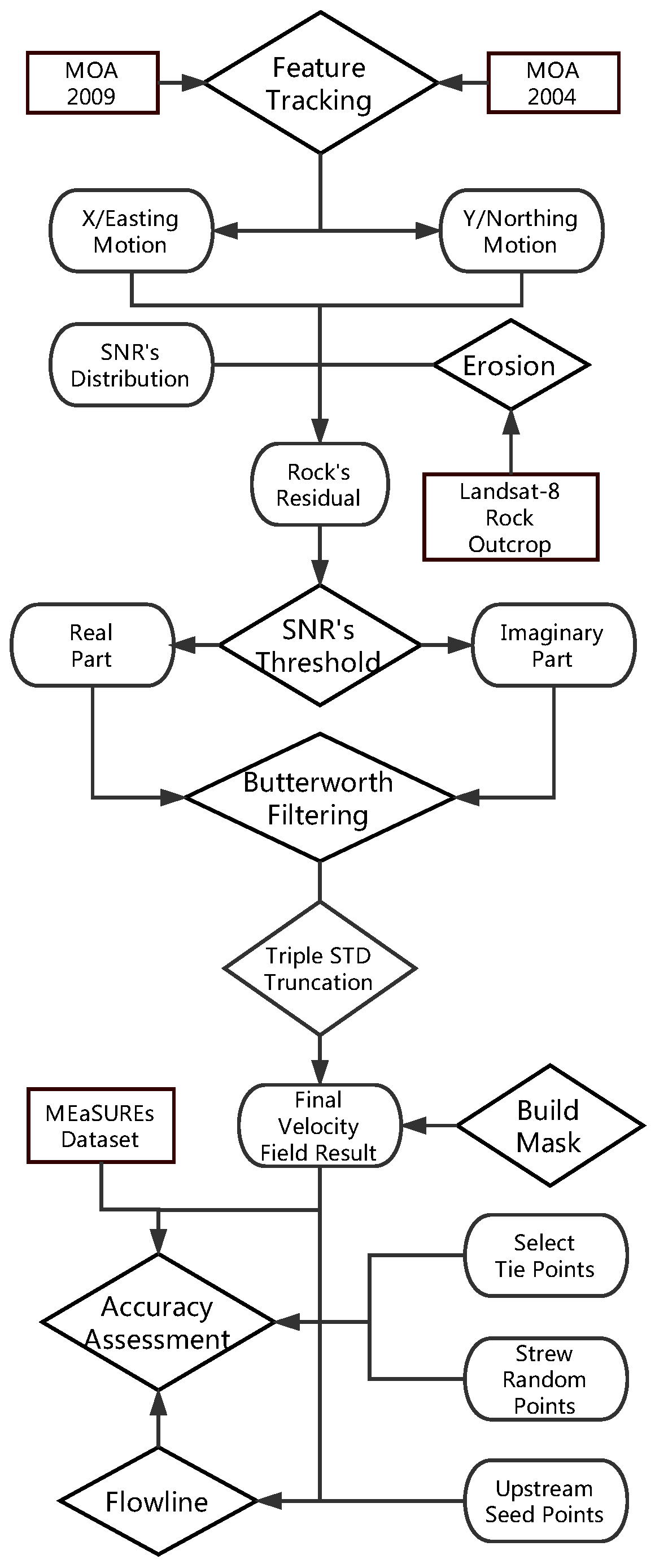
3. Methods
3.1. Feature Tracking
3.2. Post-Processing
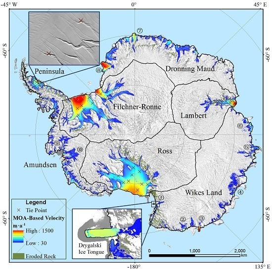
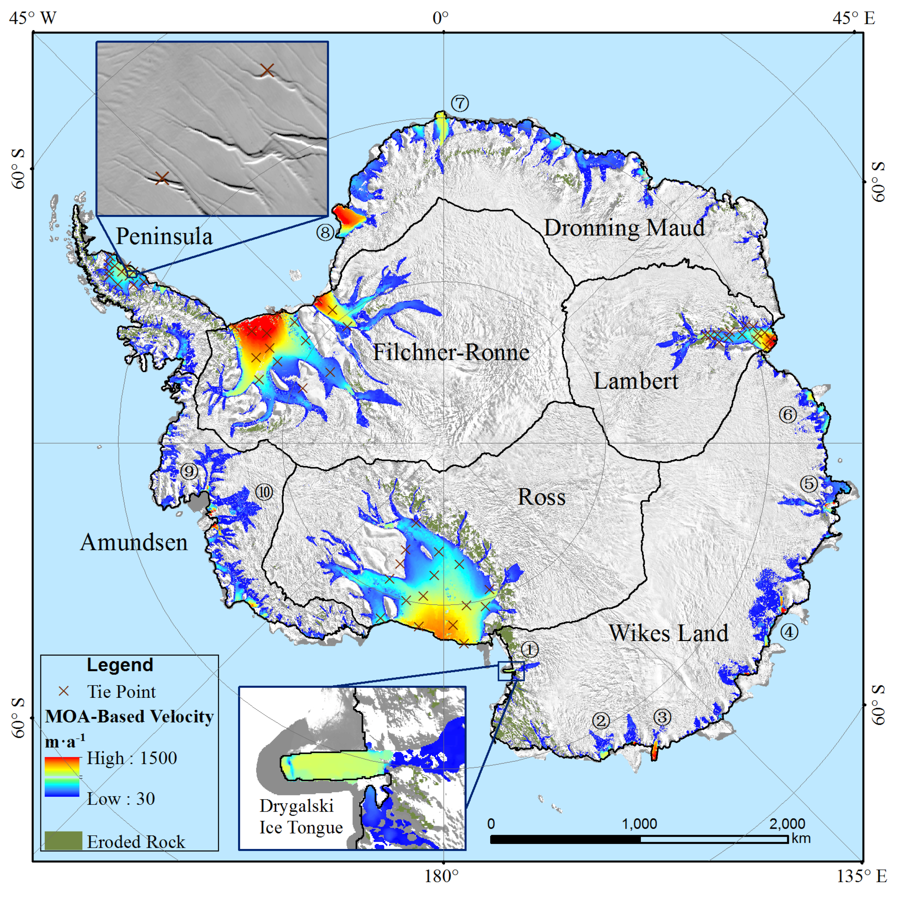
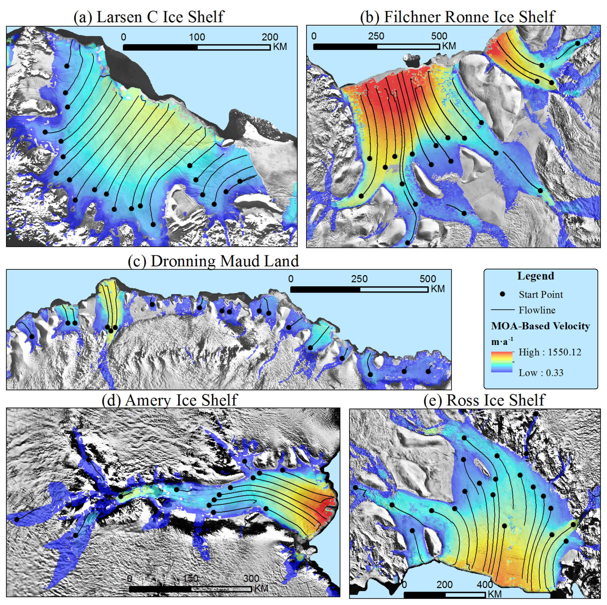
4. Result and Analysis
4.1. Streamline
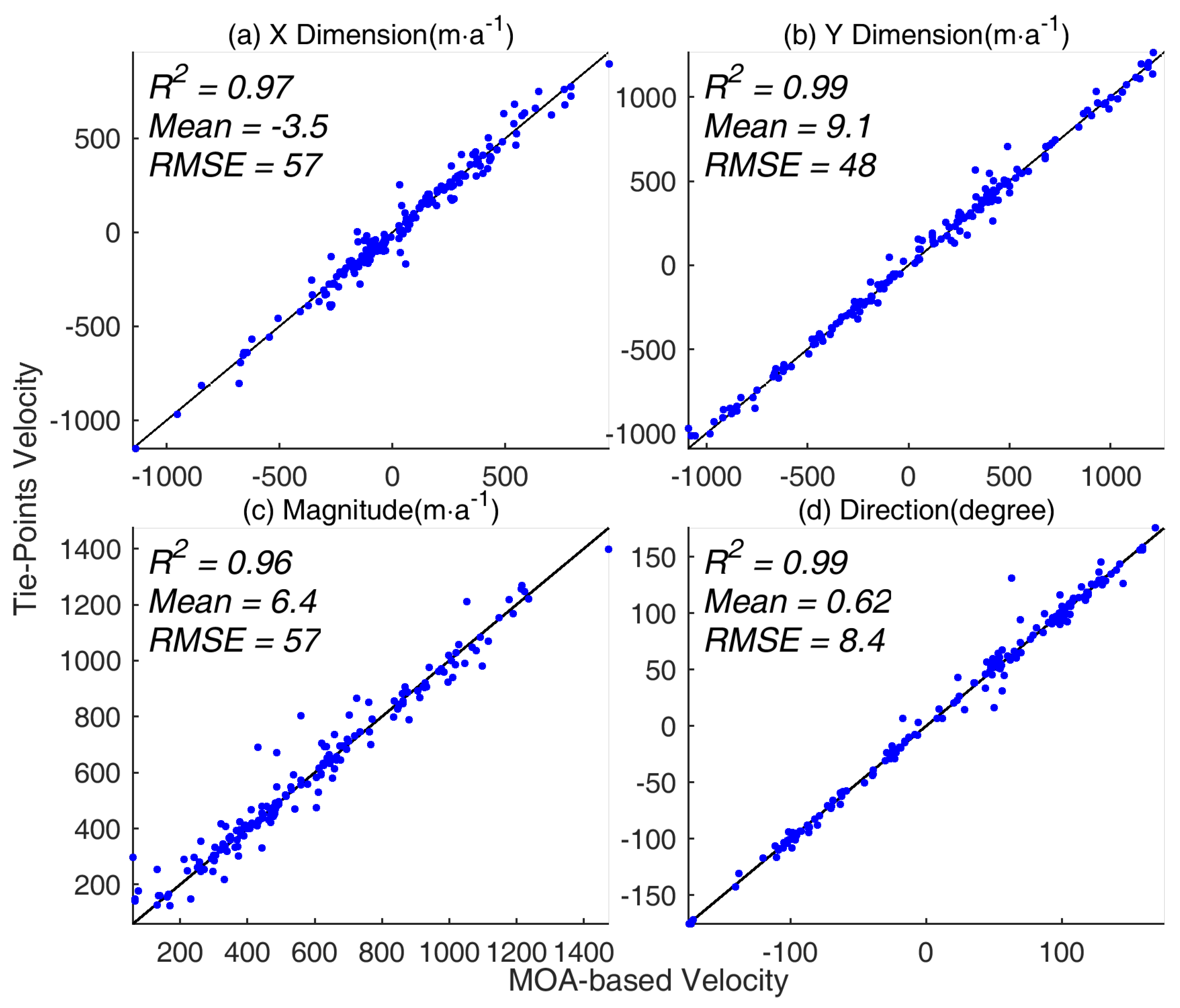
4.2. Tie Points
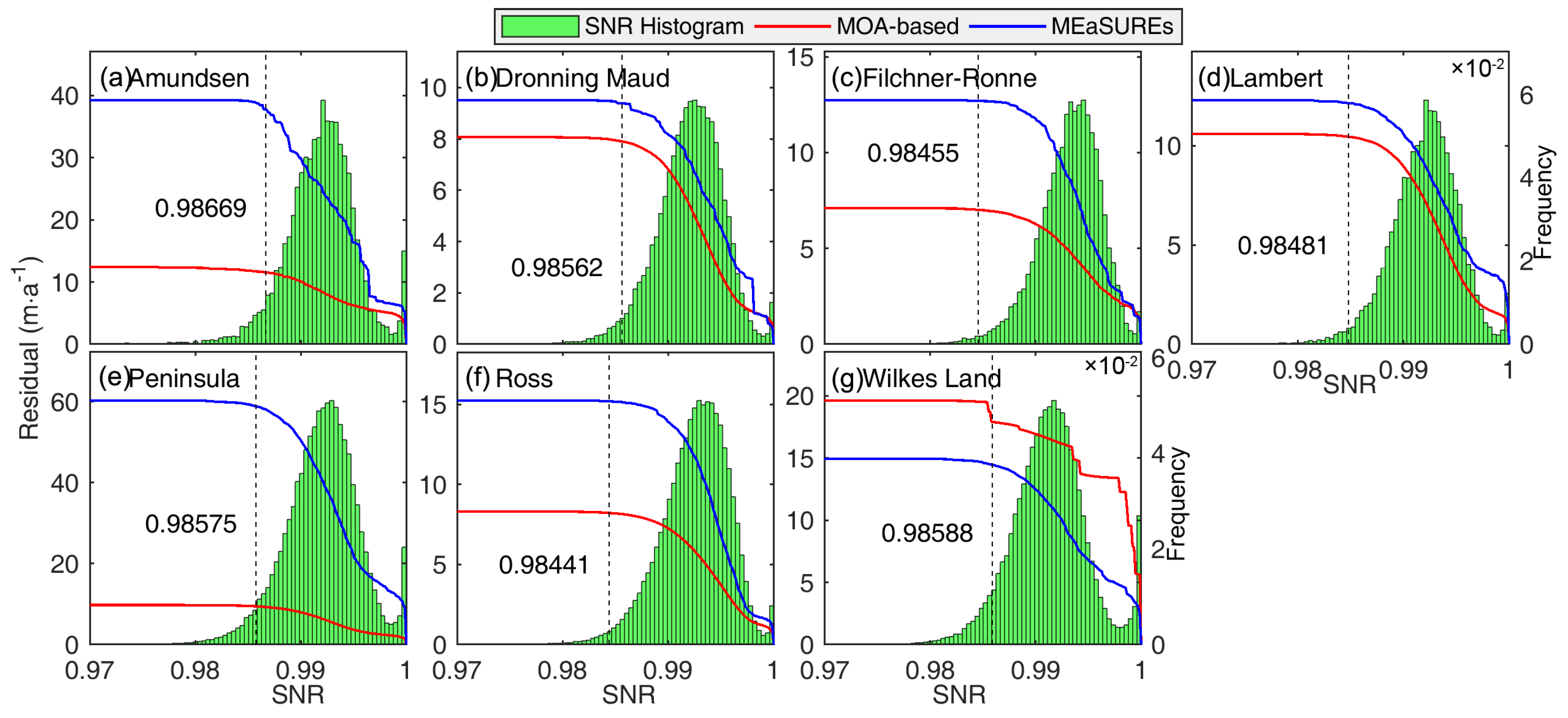
4.3. Residual in Rock Outcrop
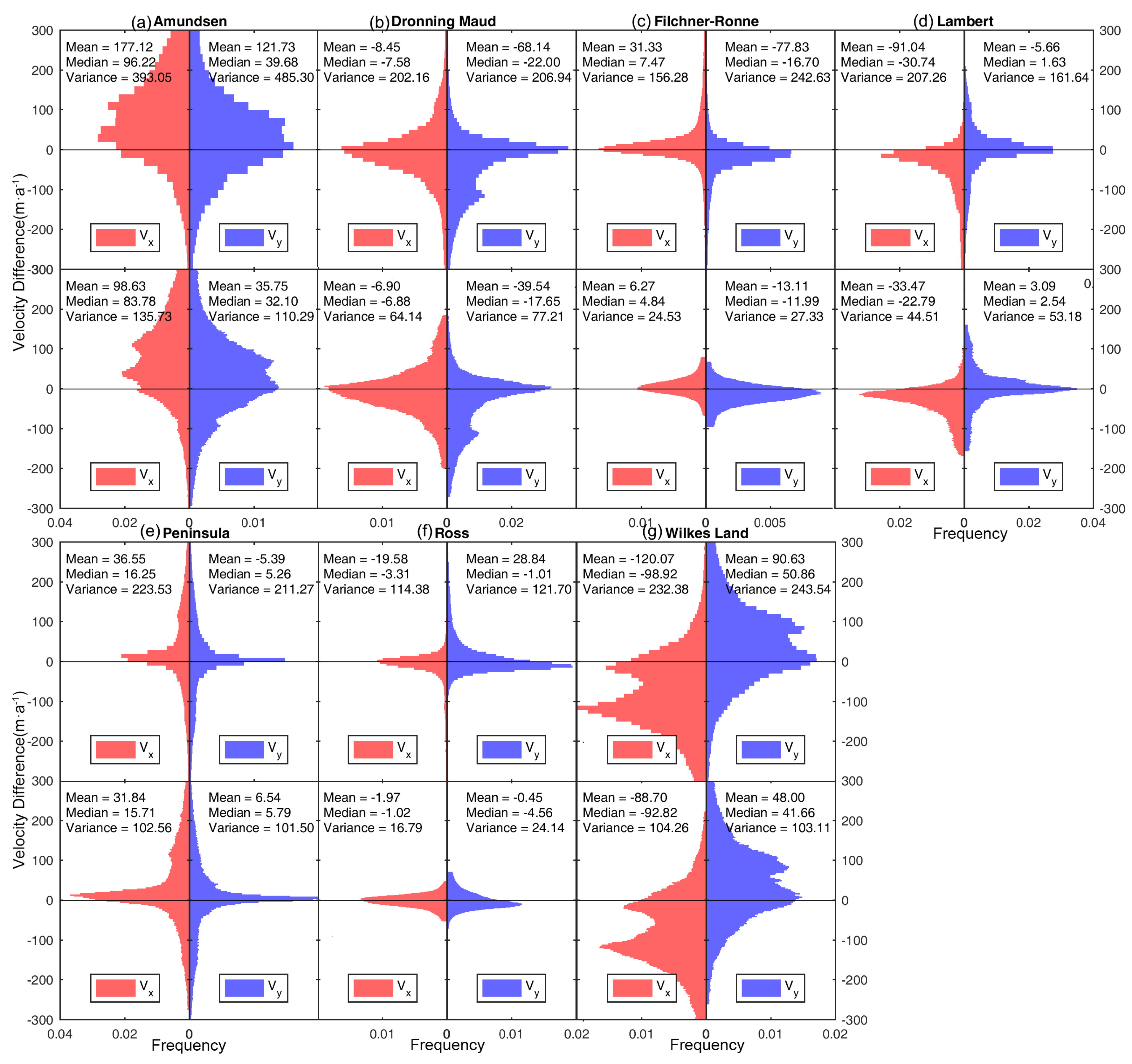
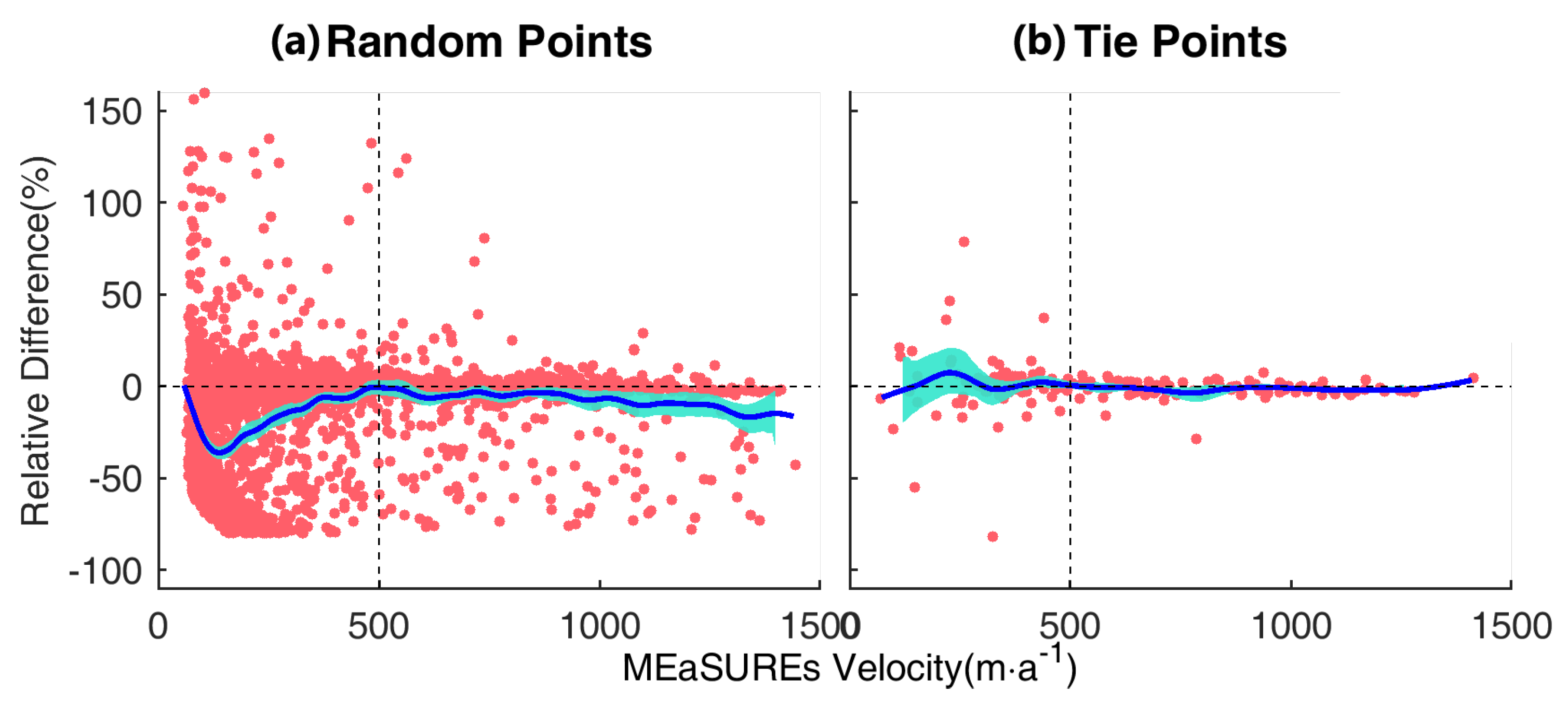
4.4. Comparisons with MEaSUREs
5. Discussion
6. Conclusions
Author Contributions
Funding
Acknowledgments
Conflicts of Interest
Abbreviations
| ADD | Antarctic Digital Database |
| ALOS | Advanced Land Observation Satellite |
| DISP | Declassified Intelligence Satellite Photography |
| EPSG | European Petroleum Survey Group |
| FFT | Fast Fourier Transform |
| ICESat | Ice, Cloud, and land Elevation Satellite |
| GHGs | Greenhouse Gases |
| GoLIVE-V1 | Global Land Ice Velocity Extraction from Landsat-8, Version 1 |
| InSAR | Interferometric Synthetic Aperture Radar |
| IPCC-AR5 | Intergovernmental Panel on Climate Change-Fifth Assessment Report |
| IPY | International Polar Year |
| MEaSUREs | Making Earth System Data Records for Use in Research Environments |
| MOA | MODIS-based Mosaic of Antarctica |
| MODIS | Moderate Resolution Imaging Spectrophotometer |
| NASA EOS | National Aeronautics and Space Administration Earth Observing System |
| NCC | Normalized Cross Correlation |
| NSIDC | National Snow and Ice Data Center |
| PALSAR | Phased Array type L-band Synthetic Aperture Radar |
| RAMP AMM-1 | Radarsat Antarctic Mapping Project Antarctic Mapping Mission 1 |
| SAR | Synthetic Aperture Radar |
| SCAR | Scientific Committee on Antarctic Research |
| SNR | Signal-to-Noise Ratio |
| UAV | Unmanned Aerial Vehicle |
References
- DeConto, R.M.; Pollard, D. Contribution of Antarctica to past and future sea-level rise. Nature 2016, 531, 591–597. [Google Scholar] [CrossRef] [PubMed]
- Krinner, G.; Magand, O.; Simmonds, I.; Genthon, C.; Dufresne, J.L. Simulated Antarctic precipitation and surface mass balance at the end of the twentieth and twenty-first centuries. Clim. Dyn. 2007, 28, 215–230. [Google Scholar] [CrossRef]
- Brigham-Grette, J.; Deconto, R.; Roychowdhury, R.; de Wet, G.; Keisling, B.; Melles, M.; Minyuk, P. Too Warm, Two Poles: Super Interglacial Teleconnections and Possible Dual Pole Ice Sheet Stability. In AGU Fall Meeting Abstracts; American Geophysical Union: Washington, DC, USA, 2017. [Google Scholar]
- Stocker, T.; Qin, D.; Plattner, G.; Tignor, M.; Allen, S.; Boschung, J.; Nauels, A.; Xia, Y.; Bex, B.; Midgley, B. Climate Change 2013: The Physical Science Basis. Contribution of Working Group I to the Fifth Assessment Report of the Intergovernmental Panel on Climate Change; Stocker, T., Qin, D., Plattner, G., Tignor, M., Allen, S., Boschung, J., Nauels, A., Xia, Y., Bex, B., Midgley, B., Eds.; Cambridge University Press: Cambridge, UK; New York, NY, USA, 1535. [Google Scholar]
- Grieger, J.; Leckebusch, G.C.; Raible, C.C.; Rudeva, I.; Simmonds, I. Subantarctic cyclones identified by 14 tracking methods, and their role for moisture transports into the continent. Tellus A Dyn. Meteorol. Oceanogr. 2018, 70, 1454808. [Google Scholar] [CrossRef]
- Simmonds, I.; Keay, K.; Lim, E.P. Synoptic Activity in the Seas around Antarctica. Mon. Weather Rev. 2003, 131, 272–288. [Google Scholar] [CrossRef]
- Scambos, T.A.; Bohlander, J.; Shuman, C.U.; Skvarca, P. Glacier acceleration and thinning after ice shelf collapse in the Larsen B embayment, Antarctica. Geophys. Res. Lett. 2004, 31, L18402. [Google Scholar] [CrossRef]
- Gardner, A.S.; Moholdt, G.; Scambos, T.; Fahnstock, M.; Ligtenberg, S.; van den Broeke, M.; Nilsson, J. Increased West Antarctic and unchanged East Antarctic ice discharge over the last 7 years. Cryosphere 2018, 12, 521. [Google Scholar] [CrossRef]
- Bingham, R.G.; Vaughan, D.G.; King, E.C.; Davies, D.; Cornford, S.L.; Smith, A.M.; Arthern, R.J.; Brisbourne, A.M.; Rydt, J.; Graham, A.G.; et al. Diverse landscapes beneath Pine Island Glacier influence ice flow. Nat. Commun. 2017, 8, 1618. [Google Scholar] [CrossRef] [PubMed]
- Scambos, T.; Bell, R.; Alley, R.; Anandakrishnan, S.; Bromwich, D.; Brunt, K.; Christianson, K.; Creyts, T.; Das, S.; DeConto, R.; et al. How much, how fast? A science review and outlook for research on the instability of Antarctica’s Thwaites Glacier in the 21st century. Glob. Planet. Change 2017, 153, 16–34. [Google Scholar] [CrossRef]
- Shen, Q.; Wang, H.; Shum, C.K.; Jiang, L.; Hsu, H.T.; Dong, J. Recent high-resolution Antarctic ice velocity maps reveal increased mass loss in Wilkes Land, East Antarctica. Sci. Rep. 2018, 8, 4477. [Google Scholar] [CrossRef] [PubMed]
- Stearns, L.A.; Smith, B.E.; Hamilton, G.S. Increased flow speed on a large East Antarctic outlet glacier caused by subglacial floods. Nat. Geosci. 2008, 1, 827–831. [Google Scholar] [CrossRef]
- Greene, C.A.; Blankenship, D.D.; Gwyther, D.E.; Silvano, A.; van Wijk, E. Wind causes Totten Ice Shelf melt and acceleration. Sci. Adv. 2017, 3, e1701681. [Google Scholar] [CrossRef] [PubMed]
- Joughin, I.; Smith, B.E.; Medley, B. Marine ice sheet collapse potentially under way for the Thwaites Glacier Basin, West Antarctica. Science 2014, 344, 735–738. [Google Scholar] [CrossRef] [PubMed]
- Liu, Y.; Moore, J.C.; Cheng, X.; Gladstone, R.M.; Bassis, J.N.; Liu, H.; Wen, J.; Hui, F. Ocean-driven thinning enhances iceberg calving and retreat of Antarctic ice shelves. Proc. Natl. Acad. Sci. USA 2015, 112, 3263–3268. [Google Scholar] [CrossRef] [PubMed]
- Bell, R.E.; Chu, W.; Kingslake, J.; Das, I.; Tedesco, M.; Tinto, K.J.; Zappa, C.J.; Frezzotti, M.; Boghosian, A.; Lee, W.S. Antarctic ice shelf potentially stabilized by export of meltwater in surface river. Nature 2017, 544, 344–348. [Google Scholar] [CrossRef] [PubMed]
- Lucchitta, B.; Ferguson, H. Antarctica: Measuring glacier velocity from satellite images. Science 1986, 234, 1105–1108. [Google Scholar] [CrossRef] [PubMed]
- Rignot, E.; Mouginot, J.; Scheuchl, B. Ice flow of the Antarctic ice sheet. Science 2011, 333, 1427–1430. [Google Scholar] [CrossRef] [PubMed]
- Mouginot, J.; Scheuchl, B.; Rignot, E. Mapping of ice motion in Antarctica using synthetic-aperture radar data. Remote Sens. 2012, 4, 2753–2767. [Google Scholar] [CrossRef]
- Heid, T.; Kääb, A. Repeat optical satellite images reveal widespread and long term decrease in land-terminating glacier speeds. Cryosphere 2012, 6, 467–478. [Google Scholar] [CrossRef]
- Mouginot, J.; Rignot, E.; Scheuchl, B.; Millan, R. Comprehensive Annual Ice Sheet Velocity Mapping Using Landsat-8, Sentinel-1, and RADARSAT-2 Data. Remote Sens. 2017, 9, 364. [Google Scholar] [CrossRef]
- Nagler, T.; Rott, H.; Hetzenecker, M.; Wuite, J.; Potin, P. The Sentinel-1 Mission: New Opportunities for Ice Sheet Observations. Remote Sens. 2015, 7, 9371–9389. [Google Scholar] [CrossRef]
- Joughin, I.; Smith, B.E.; Howat, I.M.; Scambos, T.; Moon, T. Greenland flow variability from ice-sheet-wide velocity mapping. J. Glaciol. 2010, 56, 415–430. [Google Scholar] [CrossRef]
- Dehecq, A.; Gourmelen, N.; Trouve, E. Deriving large-scale glacier velocities from a complete satellite archive: Application to the Pamir-Karakoram-Himalaya. Remote Sens. Environ. 2015, 162, 55–66. [Google Scholar] [CrossRef]
- Strozzi, T.; Paul, F.; Wiesmann, A.; Schellenberger, T.; Kääb, A. Circum-Arctic Changes in the Flow of Glaciers and Ice Caps from Satellite SAR Data between the 1990s and 2017. Remote Sens. 2017, 9, 947. [Google Scholar] [CrossRef]
- Burgess, E.W.; Forster, R.R.; Larsen, C.F. Flow velocities of Alaskan glaciers. Nat. Commun. 2013, 4, 2146. [Google Scholar] [CrossRef] [PubMed]
- Wychen, W.V.; Copland, L.; Jiskoot, H.; Gray, L.; Sharp, M.; Burgess, D. Surface Velocities of Glaciers in Western Canada from Speckle-Tracking of ALOS PALSAR and RADARSAT-2 data. Can. J. Remote Sens. 2018, 44, 57–66. [Google Scholar] [CrossRef]
- Mouginot, J.; Rignot, E. Ice motion of the Patagonian icefields of South America: 1984–2014. Geophys. Res. Lett. 2015, 42, 1441–1449. [Google Scholar] [CrossRef]
- Scheuchl, B.; Mouginot, J.; Rignot, E. Ice velocity changes in the Ross and Ronne sectors observed using satellite radar data from 1997 and 2009. Cryosphere 2012, 6, 1019–1030. [Google Scholar] [CrossRef]
- Floricioiu, D.; Jaber, W.A.; Jezek, K. TerraSAR-X and TanDEM-X observations of the Recovery Glacier system, Antarctica. In Proceedings of the 2014 IEEE International Geoscience and Remote Sensing Symposium (IGARSS), Quebec City, QC, Canada, 13–18 July 2014; pp. 4852–4855. [Google Scholar]
- Fahnestock, M.; Scambos, T.; Moon, T.; Gardner, A.; Haran, T.; Klinger, M. Rapid large-area mapping of ice flow using Landsat 8. Remote Sens. Environ. 2016, 185, 84–94. [Google Scholar] [CrossRef]
- Jeong, S.; Howat, I.M. Performance of Landsat 8 Operational Land Imager for mapping ice sheet velocity. Remote Sens. Environ. 2015, 170, 90–101. [Google Scholar] [CrossRef]
- Kääb, A.; Winsvold, S.; Altena, B.; Nuth, C.; Nagler, T.; Wuite, J. Glacier Remote Sensing Using Sentinel-2. Part I: Radiometric and Geometric Performance, and Application to Ice Velocity. Remote Sens. 2016, 8, 598. [Google Scholar] [CrossRef]
- Rosenau, R.; Scheinert, M.; Dietrich, R. A processing system to monitor Greenland outlet glacier velocity variations at decadal and seasonal time scales utilizing the Landsat imagery. Remote Sens. Environ. 2015, 169, 1–19. [Google Scholar] [CrossRef]
- Nghiem, S.V.; Hall, D.K.; Mote, T.L.; Tedesco, M.; Albert, M.R.; Keegan, K.; Shuman, C.A.; DiGirolamo, N.E.; Neumann, G. The extreme melt across the Greenland ice sheet in 2012. Geophy. Res. Lett. 2012, 39, L20502. [Google Scholar] [CrossRef]
- Key, J.R.; Santek, D.; Velden, C.S.; Bormann, N.; Thepaut, J.N.; Riishojgaard, L.P.; Yanqiu, Z.; Menzel, W.P. Cloud-drift and water vapor winds in the polar regions from MODIS. IEEE Trans. Geosci. Remote Sens. 2003, 41, 482–492. [Google Scholar] [CrossRef]
- Haran, T.; Scambos, T.; Fahnestock, M.; Yi, D.; Zwally, H. A Digital Elevation Model of West Antarctica from MODIS and ICESat: Method, Accuracy, and Applications. In AGU Fall Meeting Abstracts; American Geophysical Union: Washington, DC, USA, 2006. [Google Scholar]
- Haug, T.; Kääb, A.; Skvarca, P. Monitoring ice shelf velocities from repeat MODIS and Landsat data—A method study on the Larsen C ice shelf, Antarctic Peninsula, and 10 other ice shelves around Antarctica. Cryosphere 2010, 4, 161–178. [Google Scholar] [CrossRef]
- Chen, J.; Ke, C.; Zhou, X.; Shao, Z.; Li, L. Surface velocity estimations of ice shelves in the northern Antarctic Peninsula derived from MODIS data. J. Geogr. Sci. 2016, 26, 243–256. [Google Scholar] [CrossRef]
- Wang, S.; Liu, H.; Yu, B.; Zhou, G.; Cheng, X. Revealing the early ice flow patterns with historical Declassified Intelligence Satellite Photographs back to 1960s. Geophys. Res. Lett. 2016, 43, 5758–5767. [Google Scholar] [CrossRef]
- Li, R.; Ye, W.; Qiao, G.; Tong, X.; Liu, S.; Kong, F.; Ma, X. A New Analytical Method for Estimating Antarctic Ice Flow in the 1960s From Historical Optical Satellite Imagery. IEEE Trans. Geosci. Remote Sens. 2017, 55, 2771–2785. [Google Scholar] [CrossRef]
- Debella-Gilo, M.; Kääb, A. Measurement of Surface Displacement and Deformation of Mass Movements Using Least Squares Matching of Repeat High Resolution Satellite and Aerial Images. Remote Sens. 2012, 4, 43–67. [Google Scholar] [CrossRef]
- Berthier, E.; Vadon, H.; Baratoux, D.; Arnaud, Y.; Vincent, C.; Feigl, K.; Remy, F.; Legresy, B. Surface motion of mountain glaciers derived from satellite optical imagery. Remote Sens. Environ. 2005, 95, 14–28. [Google Scholar] [CrossRef]
- Warner, R.C.; Roberts, J.L. Pine Island Glacier (Antarctica) velocities from Landsat7 images between 2001 and 2011: FFT-based image correlation for images with data gaps. J. Glaciol. 2013, 59, 571–582. [Google Scholar] [CrossRef]
- Kääb, A. Monitoring high-mountain terrain deformation from repeated air-and spaceborne optical data: Examples using digital aerial imagery and ASTER data. ISPRS J. Photogramm. Remote Sens. 2002, 57, 39–52. [Google Scholar] [CrossRef]
- Altena, B.; Kääb, A. Glacier ice loss monitored through the Planet cubesat constellation. In Proceedings of the 2017 9th International Workshop on the Analysis of Multitemporal Remote Sensing Images (MultiTemp), Brugge, Belgium, 27–29 June 2017; pp. 1–4. [Google Scholar]
- Ryan, J.; Hubbard, A.; Box, J.; Todd, J.; Christoffersen, P.; Carr, J.; Holt, T.; Snooke, N. UAV photogrammetry and structure from motion to assess calving dynamics at Store Glacier, a large outlet draining the Greenland ice sheet. Cryosphere 2015, 9, 1–11. [Google Scholar] [CrossRef]
- Heid, T. Deriving Glacier Surface Velocities from Repeat Optical Images. Ph.D. Thesis, Oslo University, Oslo, Norway, 2011. [Google Scholar]
- Hulbe, C.L.; Scambos, T.A.; Lee, C.K.; Bohlander, J.; Haran, T. Recent changes in the flow of the Ross Ice Shelf, West Antarctica. Earth Planet. Sci. Lett. 2013, 376, 54–62. [Google Scholar] [CrossRef]
- Paul, F.; Bolch, T.; Briggs, K.; Kääb, A.; McMillan, M.; McNabb, R.; Nagler, T.; Nuth, C.; Rastner, P.; Strozzi, T.; et al. Error sources and guidelines for quality assessment of glacier area, elevation change, and velocity products derived from satellite data in the Glaciers_cci project. Remote Sens. Environ. 2017, 203, 256–275. [Google Scholar] [CrossRef]
- Altena, B.; Kääb, A.; Nuth, C. Robust glacier displacements using knowledge-based image matching. In Proceedings of the 2015 8th International Workshop on the Analysis of Multitemporal Remote Sensing Images (Multi-Temp), Annecy, France, 22–24 July 2015; pp. 1–4. [Google Scholar]
- Maksymiuk, O.; Mayer, C.; Stilla, U. Velocity estimation of glaciers with physically-based spatial regularization Experiments using satellite SAR intensity images. Remote Sens. Environ. 2016, 172, 190–204. [Google Scholar] [CrossRef]
- Scambos, T.; Haran, T.; Fahnestock, M.; Painter, T.; Bohlander, J. MODIS-based Mosaic of Antarctica (MOA) data sets: Continent-wide surface morphology and snow grain size. Remote Sens. Environ. 2007, 111, 242–257. [Google Scholar] [CrossRef]
- Burton-Johnson, A.; Black, M.; Fretwell, P.T.; Kaluza-Gilbert, J. An automated methodology for differentiating rock from snow, clouds and sea in Antarctica from Landsat 8 imagery: A new rock outcrop map and area estimation for the entire Antarctic continent. Cryosphere 2016, 10, 1665–1677. [Google Scholar] [CrossRef]
- Kang, J.; Cheng, X.; Hui, F.; Ci, T. An Accurate and Automated Method for Identifying and Mapping Exposed Rock Outcrop in Antarctica Using Landsat 8 Images. IEEE J. Sel. Top. Appl. Obs. Remote Sens. 2018, 11, 57–67. [Google Scholar] [CrossRef]
- Jawak, S.D.; Kumar, S.; Luis, A.J.; Bartanwala, M.; Tummala, S.; Pandey, A.C. Evaluation of Geospatial Tools for Generating Accurate Glacier Velocity Maps from Optical Remote Sensing Data. Proceedings 2018, 2, 341. [Google Scholar] [CrossRef]
- Leprince, S.; Barbot, S.; Ayoub, F.; Avouac, J.P. Automatic and Precise Orthorectification, Coregistration, and Subpixel Correlation of Satellite Images, Application to Ground Deformation Measurements. IEEE Trans. Geosci. Remote Sens. 2007, 45, 1529–1558. [Google Scholar] [CrossRef]
- Heid, T.; Kääb, A. Evaluation of existing image matching methods for deriving glacier surface displacements globally from optical satellite imagery. Remote Sens. Environ. 2012, 118, 339–355. [Google Scholar] [CrossRef]
- Ayoub, F.; Leprince, S.; Keene, L. User’s Guide to COSI-CORR Co-Registration of Optically Sensed Images and Correlation; California Institute of Technology: Pasadena, CA, USA, 2009; Volume 38. [Google Scholar]
- Zwally, H.J.; Giovinetto, M.B.; Beckley, M.A.; Saba, J.L. Antarctic and Greenland Drainage Systems, GSFC Cryospheric Sciences Laboratory. Available online: icesat4.gsfc.nasa.gov/cryo_data/ant_grn_drainage_systems.php. (accessed on 20 June 2018).
- Joughin, I.; Fahnestock, M.; MacAyeal, D.; Bamber, J.L.; Gogineni, P. Observation and analysis of ice flow in the largest Greenland ice stream. J. Geophys. Res. Atmos. 2001, 106, 34021–34034. [Google Scholar] [CrossRef]
- Scherler, D.; Leprince, S.; Strecker, M.R. Glacier-surface velocities in alpine terrain from optical satellite imagery-Accuracy improvement and quality assessment. Remote Sens. Environ. 2008, 112, 3806–3819. [Google Scholar] [CrossRef]
- Alley, K.E.; Scambos, T.A.; Anderson, R.S.; Rajaram, H.; Pope, A.; Haran, T.M. Continent-wide estimates of Antarctic strain rates from Landsat 8-derived velocity grids. J. Glaciol. 2018, 64, 321–332. [Google Scholar] [CrossRef]
- Han, H.; Im, J.; Kim, H. Variations in ice velocities of Pine Island Glacier Ice Shelf evaluated using multispectral image matching of Landsat time series data. Remote Sens. Environ. 2016, 186, 358–371. [Google Scholar] [CrossRef]
- Wang, X.; Holland, D.M.; Cheng, X.; Gong, P. Grounding and calving cycle of Mertz Ice Tongue revealed by shallow Mertz Bank. Cryosphere 2016, 10, 2043–2056. [Google Scholar] [CrossRef]
- Massom, R.; Lubin, D. Polar Remote Sensing; Springer: Chichester, UK, 2006; Volume 2, p. 262. [Google Scholar]
- Gray, A.; Short, N.; Mattar, K.; Jezek, K. Velocities and flux of the Filchner Ice Shelf and its tributaries determined from speckle tracking interferometry. Can. J. Remote Sens. 2001, 27, 193–206. [Google Scholar] [CrossRef]
- Altena, B.; Kääb, A. Elevation change and improved velocity retrieval using orthorectified optical satellite data from different orbits. Remote Sens. 2017, 9, 300. [Google Scholar] [CrossRef]
- Konrad, H.; Shepherd, A.; Gilbert, L.; Hogg, A.E.; McMillan, M.; Muir, A.; Slater, T. Net retreat of Antarctic glacier grounding lines. Nat. Geosci. 2018, 11, 258. [Google Scholar] [CrossRef]
- Christianson, K.; Bushuk, M.; Dutrieux, P.; Parizek, B.R.; Joughin, I.R.; Alley, R.B.; Shean, D.E.; Abrahamsen, E.P.; Anandakrishnan, S.; Heywood, K.J.; et al. Sensitivity of Pine Island Glacier to observed ocean forcing. Geophys. Res. Lett. 2016, 43, 10817–10825. [Google Scholar] [CrossRef]
- Kääb, A. Combination of SRTM3 and repeat ASTER data for deriving alpine glacier flow velocities in the Bhutan Himalaya. Remote Sens. Environ. 2005, 94, 463–474. [Google Scholar] [CrossRef]
- Kääb, A.; Lefauconnier, B.; Melvold, K. Flow field of Kronebreen, Svalbard, using repeated Landsat 7 and ASTER data. Ann. Glaciol. 2005, 42, 7–13. [Google Scholar] [CrossRef]
- Joughin, I. Ice-sheet velocity mapping: A combined interferometric and speckle-tracking approach. Ann. Glaciol. 2002, 34, 195–201. [Google Scholar] [CrossRef]
- Yan, Y.; Dehecq, A.; Trouve, E.; Mauris, G.; Gourmelen, N.; Vernier, F. Fusion of Remotely Sensed Displacement Measurements: Current status and challenges. IEEE Geosci. Remote Sens. Mag. 2016, 4, 6–25. [Google Scholar] [CrossRef]
- Lüttig, C.; Neckel, N.; Humbert, A. A Combined Approach for Filtering Ice Surface Velocity Fields Derived from Remote Sensing Methods. Remote Sens. 2017, 9, 1062. [Google Scholar] [CrossRef]
- Liu, T.; Niu, M.; Yang, Y. Ice Velocity Variations of the Polar Record Glacier (East Antarctica) Using a Rotation-Invariant Feature-Tracking Approach. Remote Sens. 2018, 10, 42. [Google Scholar] [CrossRef]


© 2018 by the authors. Licensee MDPI, Basel, Switzerland. This article is an open access article distributed under the terms and conditions of the Creative Commons Attribution (CC BY) license (http://creativecommons.org/licenses/by/4.0/).
Share and Cite
Li, T.; Liu, Y.; Li, T.; Hui, F.; Chen, Z.; Cheng, X. Antarctic Surface Ice Velocity Retrieval from MODIS-Based Mosaic of Antarctica (MOA). Remote Sens. 2018, 10, 1045. https://doi.org/10.3390/rs10071045
Li T, Liu Y, Li T, Hui F, Chen Z, Cheng X. Antarctic Surface Ice Velocity Retrieval from MODIS-Based Mosaic of Antarctica (MOA). Remote Sensing. 2018; 10(7):1045. https://doi.org/10.3390/rs10071045
Chicago/Turabian StyleLi, Teng, Yan Liu, Tian Li, Fengming Hui, Zhuoqi Chen, and Xiao Cheng. 2018. "Antarctic Surface Ice Velocity Retrieval from MODIS-Based Mosaic of Antarctica (MOA)" Remote Sensing 10, no. 7: 1045. https://doi.org/10.3390/rs10071045
APA StyleLi, T., Liu, Y., Li, T., Hui, F., Chen, Z., & Cheng, X. (2018). Antarctic Surface Ice Velocity Retrieval from MODIS-Based Mosaic of Antarctica (MOA). Remote Sensing, 10(7), 1045. https://doi.org/10.3390/rs10071045