Mapping Vegetation and Land Use Types in Fanjingshan National Nature Reserve Using Google Earth Engine

Abstract

Fanjingshan National Nature Reserve (FNNR) is a biodiversity hotspot in China that is part of a larger, multi-use landscape where farming, grazing, tourism, and other human activities occur. The steep terrain and persistent cloud cover pose challenges to robust vegetation and land use mapping. Our objective is to develop satellite image classification techniques that can reliably map forest cover and land use while minimizing the cloud and terrain issues, and provide the basis for long-term monitoring. Multi-seasonal Landsat image composites and elevation ancillary layers effectively minimize the persistent cloud cover and terrain issues. Spectral vegetation index (SVI) products and shade/illumination normalization approaches yield significantly higher mapping accuracies, compared to non-normalized spectral bands. Advanced machine learning image classification routines are implemented through the cloud-based Google Earth Engine platform. Optimal classifier parameters (e.g., number of trees and number of features for random forest classifiers) were achieved by using tuning techniques. Accuracy assessment results indicate consistent and effective overall classification (i.e., above 70% mapping accuracies) can be achieved using multi-temporal SVI composites with simple illumination normalization and elevation ancillary data, despite the fact limited training and reference data are available. This efficient and open-access image analysis workflow provides a reliable methodology to remotely monitor forest cover and land use in FNNR and other mountainous forested, cloud prevalent areas.

1. Introduction

Despite their protected status, nature reserves can be strongly influenced by adjacent or overlapping anthropogenic activities [1]. Given this sensitivity, accurately mapping vegetation community and land use types is important to maintain the integrity of reserve habitat and biodiversity. Fanjingshan National Nature Reserve (FNNR), a national forest reserve in Guizhou province, China, has been identified as one of the 25 global biodiversity hotspots [2] with over 100 endemic species. However, human activities such as farming, grazing, tourism, and related development frequently occur from the 21,000 people living within or near the Reserve [3].

To protect ecosystem services (limiting soil erosion and runoff) and FNNR biodiversity, Chinese government agencies have implemented payment for ecosystem services (PES) policies to promote afforestation, reduce logging, and limit farming on high sloping lands surrounding the Reserves [4,5,6]. Such PES programs include the National Forest Conservation Program (NFCP) in 1998, which seeks to ban logging and promote afforestation to restore forests through incentives paid to forest enterprises or users. One year later, China started another large PES program, the Grain-To-Green Program (GTGP). This program aims to reduce soil erosion and increase vegetation cover through tree planting in steep farmland areas (>15° slope in northwestern China, and 25° in southwestern China; [7,8]). This context makes monitoring and mapping forest vegetation and land use types an essential element of such programs. At FNNR, these two programs have been implemented for over 16 years, yet quantitative, large scale data about PES effectiveness remains scarce. The reserve management would benefit from mapping and monitoring forest composition and cover in a reliable and extensive manner. While the most feasible and efficient means for such mapping and monitoring is through satellite remote sensing, the persistent cloud cover and steep terrain associated with the FNNR region pose a great challenge to forest mapping with optical or microwave remote sensing approaches.

Landsat satellite imagery has several characteristics that can support long-term mapping and monitoring of vegetation and land cover changes. Landsat systems provide regular image collection at 30 m spatial resolution with a potential frequency of every 16 days and a freely available image archive dating to the early- to mid-1980s [9]. More stable and reliable land change analyses with multi-temporal Landsat data are enabled when digital numbers are converted to surface reflectance values. The conversion to surface reflectance accounts for some atmospheric and solar illumination effects and ensures multi-date images are more comparable [10,11]. Landsat surface reflectance products are processed through algorithms of the Landsat Ecosystem Disturbance Adaptive Processing System (LEDAPS; [12]) for Landsat 4, 5, and 7, and Landsat Surface Reflectance Code (LaSRC) for Landsat 8 imagery.

Spectral vegetation indices (SVIs) are commonly derived from multispectral images to characterize vegetation. Normalized indices such as simple ratio, normalized difference vegetation index (NDVI), and enhanced vegetation index (EVI) can partially suppress illumination, terrain, and soil reflectance influences in the image data to more reliably monitor vegetation [13]. For example, EVI was found to be resilient to residual atmospheric effects in a recent study [14]. Modified soil adjusted vegetation index (MSAVI) and EVI contain a soil adjustment factor that minimizes the soil background while increasing the range of vegetation signal [13]. MSAVI demonstrated the most linear relationship when regressed with biomass in the Amazonian region among the commonly utilized SVIs [15]. However, in mountainous regions, the soil adjustment factor was found to cause EVI to be more sensitive to topographic effects when comparing to NDVI [16].

Compositing or exploiting dense layer stacks of multi-temporal images have been demonstrated to improve forest and land use type mapping accuracy [17]. Images can be composited to form a multi-layer time series stack to map forest cover, whether they are from the same or different seasons. By compositing multiple images, clouds, and other missing data that occur in single images can be ignored, and seasonal phenology signals may be exploited [18]. Potapov [19] found that Landsat composites of the growing season ensured anomaly-free pixels, and were effective in mapping boreal forest cover and change. Forest types were successfully mapped with multi-date Landsat images in New Hampshire [20] and Wisconsin [21], with accuracies of 74% and 83%, respectively. Including ancillary data during the classification has also been found to improve classification accuracy [9,22,23]. In a steep mountainous study area, Dorren et al. mapped forest types using Landsat Thematic Mapper data and a digital elevation model (DEM) layer to account for variable illumination effects, with a 73% overall accuracy [24].

Machine learning type classifiers may require larger amounts of training data [25], but higher mapping accuracy can also be achieved than conventional classifiers [26]. A variety of machine learning image classification methods have been used to map vegetation type and land use, such as artificial neural networks (NN), support vector machine (SVM), decision tree (i.e., CART), and random forest classifiers. SVM classifiers assign pixels to classes by maximizing class separability from the training data, and labels pixels according to their nearest class in feature space [27,28]. Decision tree classifiers [29] apply a multi-stage binary decision making system to classify images. At each stage, pixels are divided according to the binary classification rule. Groups of pixels can be further divided based on tree growing and pruning parameters, until optimal classification is achieved. Decision tree models can be sensitive to small changes to the training data and parameters [30]. Random forest classifiers construct a multitude of decision trees that are sampled independently during training, typically improving classification results over a single decision tree model [31,32]. These machine learning classifiers require various input parameters, which can be optimized through cross-validation. In a previous study on the classification of natural vegetation in the Mediterranean region, Sluiter and Pebesma [22] utilized HyMap, ASTER optical bands, and Landsat 7 images and found that machine learning classifiers yielded up to 75% accuracy and outperformed conventional statistical-based classifiers. Johansen et al. [33] mapped woody vegetation in Australia using Landsat 5 and 7 images, and concluded that CART and random forest classifiers produced highly accurate vegetation change maps. A study on crop and land cover mapping in Ukraine compared different machine learning image classifiers, with the highest map accuracy (~75%) achieved with CART [32]. With a random forest classifier and MODIS data, Parente et al. [34] achieved almost 80% accuracy when mapping pastureland in Brazil. Other studies conclude that random forest classifiers yield higher classification accuracies, require less model training time, and are less sensitive to training sample qualities compared to SVM and NN classifiers [35,36].

Cloud-computing resources enable efficient image processing on otherwise computational intensive tasks, such as with classification of large volumes of image data, and particularly when using advanced machine learning algorithm. Google Earth Engine (https://earthengine.google.com/) is a cloud-based platform for geospatial analysis [37] that is open-access and free of charge for research, education, and non-profit purposes. The platform requires a simple online application and a Google user account to access. With a JavaScript code editor platform, Earth Engine provides a massive imagery data collection (including almost the entire Landsat archive and associated surface reflectance products) that can be retrieved directly, allowing users to interactively test and develop algorithms and preview results in real time. Earth Engine also provides various pixel-based supervised and unsupervised classifiers, including machine learning type algorithms, for mapping implementation. Google Earth Engine was utilized by Hansen et al. [38] to generate global forest cover change products. Over 650 thousand Landsat 7 scenes were incorporated, and the processes took just a few days. Other studies have also demonstrated the ease of incorporating various sources of imagery data and automating image classification routines for crop and vegetation mapping using Earth Engine [32,33,34].

The objective of this study is to develop and test advanced image classification techniques on the cloud-based platform Google Earth Engine for mapping vegetation and land use types in the FNNR region, and analyze their spatial distributions. A secondary objective is to determine if multi-temporal composites, SVIs, and digital elevation data enable more accurate forest and land cover mapping results in this cloud prone and complex terrain study area. Tree-based machine learning image classifiers—decision tree and random forest classifiers—are applied to multi-temporal Landsat data to generate vegetation and land cover maps. Cloud-free multi-seasonal image composites consisting of spectral vegetation indices (SVI) and ancillary data are tested for effectiveness in vegetation type mapping. Terrain shading normalization approaches are implemented to improve the mapping results in the mountainous study area. Vegetation type maps are assessed for accuracy by comparison with reference data collected through field assessment with sampling plots. The vegetation and land use mapping workflow, which includes cloud-based image processing approaches, provides a reliable method to remotely map forest and land use composition in FNNR.

2. Study Area and Materials

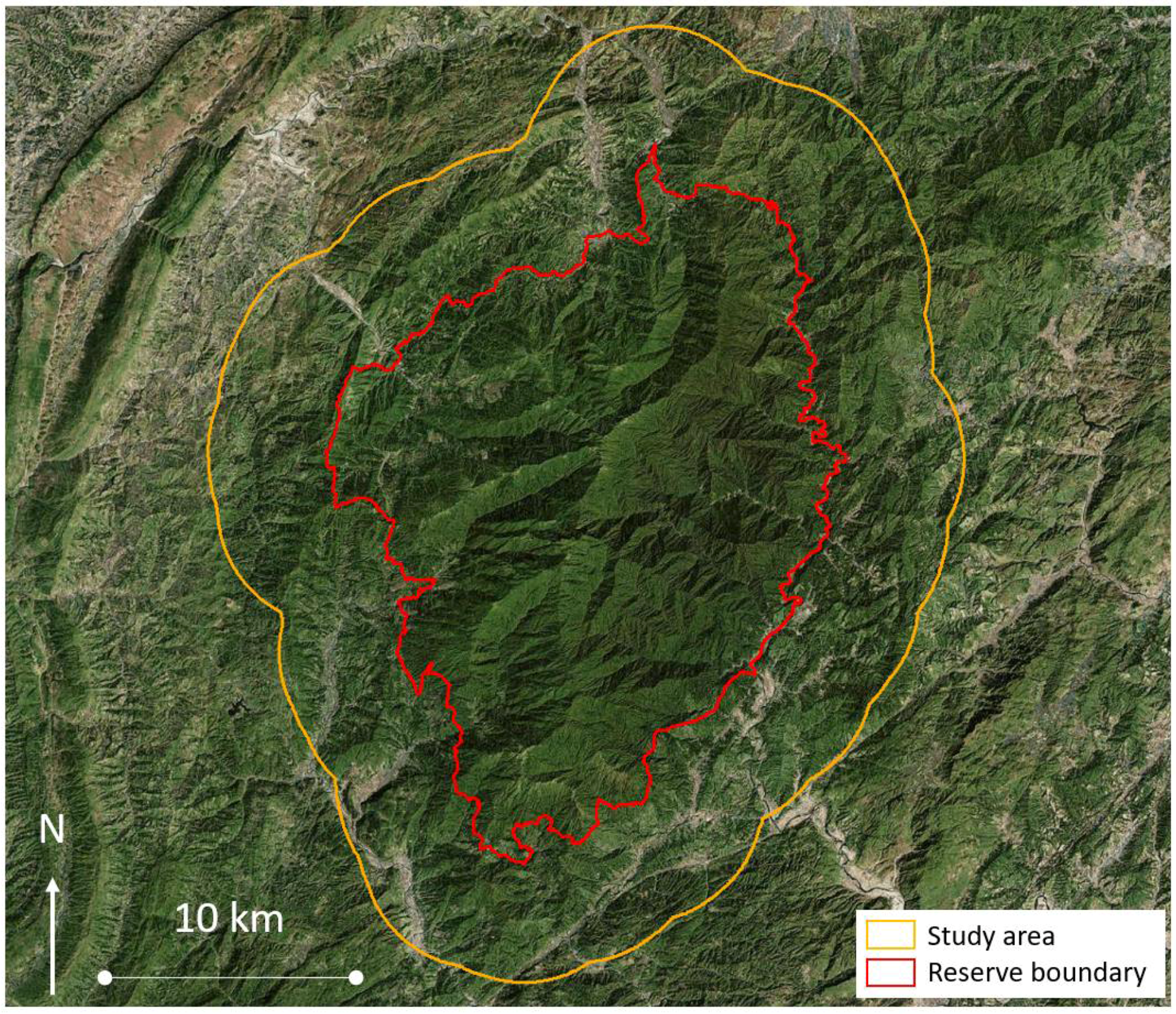
Fanjingshan National Nature Reserve (FNNR, 27.92°N, 108.70°E), as shown in Figure 1, is roughly 419 km² in size. FNNR was established in 1978 as a protected area, and was included in the UNESCO Man and Biosphere Protection network in 1986. The mountainous terrain displays a vertical elevation difference of over 2000 m, and is located in the humid subtropical climate zone. FNNR is also referred to as “ecosystem kingdom”, because of its diverse microclimate that creates habitat for over 6000 different types of plants and animals, and over 100 endemic species. The vegetation communities of the FNNR region are complex and normally mixed, and almost no single-species cover type exists [39]. Based on the dominant species, we generalized the vegetation communities into five common types for this study: deciduous, evergreen broadleaf, mixed deciduous and evergreen, bamboo, and conifer. Non-reserve land use types, namely built and terraced agriculture, tend to be located along the periphery of the forest reserve.

Landsat 5 Thematic Mapper (TM) and Landsat 8 Operational Land imager (OLI) surface reflectance images of FNNR (located within Worldwide Reference System 2 path 126, row 41) on the USGS Earth Explorer website (EarthExplorer, http://earthexplorer.usgs.gov) were reviewed, and selected dates were retrieved from the Google Earth Engine image library for image processing and analysis. Landsat 7 Enhanced Thematic Mapper Plus (ETM+) images were not utilized for this study due to the Scan Line Corrector failure since 2003. Based on cloud cover and image availability for coverage throughout a vegetation growing season, two study years were selected for this study, 2011 and 2016. Images were also visually inspected to ensure the quality of the analysis.

Table 1. Image dates and number of images associated with the study periods for this study.

Study Period & Sensor	Image Dates
	Single Summer Date	Cloud-Free Layerstack	Seasonal Composite
Circa 2011 Landsat 5	16 August 2011	1 November 2010 28 May 2011 16 August 2011	2010–2011 13 images
Circa 2016 Landsat 8	29 August 2016	14 October 2015 29 August 2016 28 May 2017	2015–2016 17 images

provides information on specific image dates, sensors, and number of images used.

The FNNR study area is extremely mountainous and cloud-prone. We evaluated the cloud cover statistics with the C version of Function of Mask products (CFmask; [40]) provided with the Landsat LEDAPS/LaSRC processed data sets. Landsat imagery for both study periods contains persistent cloud cover. For the circa 2011 period, portions of the study area have up to ten out of 13 available images that were covered by clouds. A minimum of eight image dates out of 17 images for the circa 2016 period have high amounts of cloud cover. For areas such as the highest ridge and peak located at above 2560 m elevation, there was only one image during the latter study period that provided cloud-free coverage. As Table 1 shows, two mostly cloud-free August images were selected to analyze single-date classification accuracies for 2011 and 2016. Two types of multi-temporal image stacks were also generated for the study periods: cloud-free layerstacks and seasonal composites. The compositing method is described in Section 3.1.

Ground reference data on vegetation composition within the portions of the FNNR were collected during Fall 2012, Spring 2013, Spring 2015, Fall 2015, and Spring 2016. Relatively homogeneous 20 × 20 m² and 30 × 30 m² areas were chosen as survey plots, on the ground, based on accessibility and visual inspection. Survey plot locations were selected to ensure sampling within the five common vegetation types in FNNR—deciduous, evergreen broadleaf, mixed deciduous and evergreen, bamboo, and conifer. At every plot, we determined the dominant vegetation community type based on species cover through a rapid assessment process similar to the California Native Plant Society’s Rapid Assessment Protocol [41]. We also collected digital photographs and vegetation structure information. All the survey plot locations were recorded with a global navigation satellite system receiver.

The survey locations were recorded often under the dense vegetation cover in the mountainous terrain in the study area. These factors led to difficulty in collecting more reference data, and led to a higher degree of uncertainty in positional accuracy. Prior to utilizing the survey data points, we improved the reliability of the reference dataset by cross validating with an unpublished vegetation community map. The vegetation community map was created through a collaborative project between Global Environmental Facility (GEF) and the FNNR management office in 2007. This map was generated through the combination of forest inventory field surveys and visual interpretation of a Landsat image. The map depicted 37 dominant overstory species for the reserve and was rendered to the five common FNNR vegetation community types (i.e., deciduous, evergreen, mixed deciduous and evergreen, bamboo, and conifer). While we use the map as additional reference data, the accuracy of the map has not been determined and we have observed errors when comparing the map to high spatial resolution satellite imagery. The locations and vegetation types of the survey data samples were cross-validated and co-located with the GEF 2007 vegetation map. When field assessment and map data did not agree, vegetation type classes were determined using other reference sources, such as PES locations derived from household surveys, high spatial resolution Google Earth images (namely 2013 and 2017 Pleiades), and ArcGIS Basemap imagery (pan-sharpened QuickBird, GeoEye, and WorldView-2 images from 2004 to 2012).

3. Methods

The majority of the image processing and analysis for this study was implemented through Google Earth Engine. The methods include image normalization for illumination effects (i.e., shade), generating multi-seasonal image stacks, tuning machine learning classifier parameters, generating classification maps, and assessing accuracies of vegetation/land use products.

3.1. Multi-Temporal Image Stacks

Two types of multi-temporal image stacks were generated: cloud-free layerstacks, and seasonal composites. The cloud-free layerstack image input was formed by stacking the most cloud-free Spring and Fall images available within two consecutive years of the selected Summer image. Images were combined to form a three-date stack. To minimize cloud pixels, seasonal image composites were also generated. For the seasonal composites, all Landsat images that were captured during the years of 2010–2011, and 2015–2016 were utilized. In order for the composites to preserve seasonal vegetation signals, we split the images into Spring, Summer, and Fall season groups. For each seasonal group, the mean value between all available images was calculated. Lastly, the three season layers were combined (i.e., layerstacked) to form the seasonal composites.

3.2. Classification Feature Input

Due to the extreme elevation range and steep slopes in the FNNR region, a reflectance normalization process was applied to Landsat images by dividing each reflectance band by the reflectance sum of all bands [42]. Spectral band derivatives were utilized to further minimize terrain illumination effects and maximize vegetation signature differences. Six SVI derived from the reflectance normalized Landsat spectral bands, along with elevation, slope, and aspect layers derived from a SRTM DEM were used as feature inputs for vegetation and land use classification. The slope layer was calculated in degrees, ranging from 0 to 90°. The aspect layer had a value range from 0 to 360°, and was transformed by taking the trigonometric sine values of aspect to avoid circular data values [43]. Sine values of aspect represents the degree of east-facing slopes, as the values range from 1 (i.e., east-facing) to −1 (west-facing). Clouds, cloud shadow, and water bodies were masked using the CFmask products.

NDVI, normalized difference blue and red (NDBR), normalized difference green and red (NDGR), normalized difference shortwave infrared and near infrared (NDII), MSAVI, and spectral variability vegetation index (SVVI) were derived from the Landsat data as defined below. MSAVI is calculated as Equation (1) [13]:

$$\mathrm{MSAVI}= \frac{2{\rho }_{\mathrm{NIR}}+1- \sqrt{{\left(2{\rho }_{\mathrm{NIR}}+1\right)}^2-8\left({\rho }_{\mathrm{NIR}}- {\rho }_{\mathrm{red}}\right)}}{2}$$

(1)

NDVI is calculated as Equation (2) [44]:

$$\mathrm{NDVI}= \frac{{\rho }_{\mathrm{NIR}} - {\rho }_{\mathrm{red}}}{{\rho }_{\mathrm{NIR}} + {\rho }_{\mathrm{red}}}$$

(2)

where ρ_NIR and ρ_red in Equations (1) and (2) represent the near infrared and red reflectance values for a given pixel. The other three normalized difference indices: NDBR, NDGR, and NDII, were calculated as the form of NDVI in Equation (2), only with blue and red bands for NDBR, green and red bands for NDGR, and infrared bands (NIR and SWIR) for NDII. SVVI is calculated as the difference between the standard deviation (SD) of all Landsat bands (excluding thermal) and SD of all three infrared bands, as displayed in Equation (3) [45]:

$$\mathrm{SVVI}=SD\left({\rho }_{all bands}\right)-SD\left({\rho }_{NIR and SWIR}\right)$$

(3)

3.3. Classifiers

Two pixel-based, supervised machine learning type image classifiers were implemented and tested: decision tree (DT) and random forest (RF). To train and test the image classifiers, we utilized the forest composition survey data and manually digitized agriculture and built sample areas based on high spatial resolution satellite imagery. We derived a total of 109 samples for image classifier training and testing purposes. Of the 109 samples, 34 represented mixed, 12 broadleaf, and eight deciduous vegetation, 16 conifer, 10 bamboo, six bare land, 11 agriculture, and 12 built land uses. These samples were stratified by image illumination to account for the drastic spectral difference between illuminated and shaded slopes [46]. We organized the samples in a Google Fusion Table and retrieved in Google Earth Engine. The corresponding input image values for the 109 samples were extracted at the Landsat image pixel level.

Cross-validation and grid search techniques were implemented to optimize classifier parameters and ensure model fitting. The 109 samples were randomly selected and split into two parts (i.e., cross-validation): 2/3 for training and 1/3 for testing. Samples were selected by each class to maintain the class proportion. Different combinations of classifier parameters were systematically tested (i.e., grid search) with the training samples. The trained models were then evaluated using the reserved 1/3 testing samples for the estimated model performance. The parameter combination that yielded the highest testing accuracy was used as the optimal classifier parameter. Final vegetation and land use maps were produced based on the optimal classifier parameters utilizing the entire set of data samples. The derived maps portray the five vegetation types (bamboo, conifer, deciduous, evergreen broadleaf, and mixed deciduous and evergreen) and three land use types: agriculture, bare soil, and built.

3.4. Accuracy Assessment

The classification products were evaluated for mapping accuracy using an independent set of accuracy data points. We had difficulties discerning certain forest community types. Thus, the seven-class mapping scheme was generalized into four classes—built, agriculture, forest, and bamboo/conifer vegetation to create a second, more generalized map as part of the accuracy assessment. Conifer and bamboo were grouped into a single class, while the forest class contained deciduous, evergreen, and mixed deciduous and evergreen. A total of 128 points (32 points per class) for the study area were generated using a distance-restricted random method (i.e., points to be at least five Landsat pixels apart) and manual editing. Points were overlaid on the Planet imagery captured on July 2017 [47] and manually labeled as forest, bamboo/conifer, agriculture, or built class. The labeled reference points were compared to the corresponding classified pixels, and the percent of agreement was recorded in an accuracy table.

To examine the forest community type classification accuracy, the Landsat-derived classification products for 2011 were compared to the 2007 GEF vegetation map. A spatial correspondence matrix was generated for each product to quantify the site-specific and areal coverage similarities and differences between the classification maps and the GEF map. Only the 2011 classification maps were evaluated for they correspond in time better with the GEF map.

Classification products from the same time period that were derived using different inputs and classifiers were also compared to each other to evaluate differences in classifiers and how they represented the vegetation and land use of the study area. The most reliable classification approach was determined based on mapping accuracies, and the map comparison and evaluation results between the GEF map and the circa 2011 classification products.

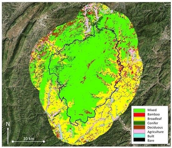
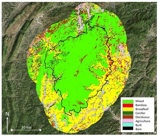
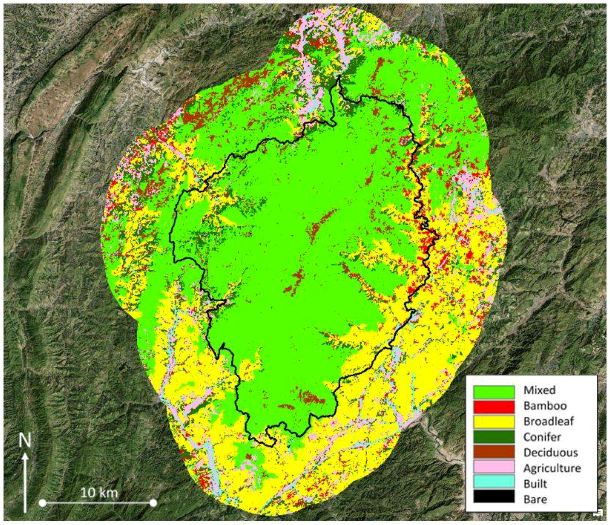
4. Results

Figure 2 shows the circa 2016 classification map using RF classifier with the seasonal composite image inputs. The reserve is mostly classified as mixed evergreen and deciduous type (displayed in light green color in Figure 2). Evergreen broadleaf cover (displayed in yellow) has a distinct distribution along the river and stream channels that originate from the reserve, in addition to the concentration on the eastern and southern side of the study area. Deciduous cover type (displayed in brown) is concentrated along the high elevation ridge in the middle of the reserve, as well as the two clusters found on the south end. As for the bamboo and conifer vegetation types, more bamboo cover (displayed in red) is mapped on the eastern side of the reserve, and conifer (displayed in dark green) were found more concentrated to the west and north. The road network that surrounds the reserve is depicted as part of the built class. Mapped in close proximity to built areas are agriculture land, bamboo, and conifer cover types. They are found distributed towards the periphery and outside of the reserve boundary.

Key image classifier parameters were tuned for optimizing the classification accuracies. Optimal parameters were identified for each study period and image input type, and they can be found in

Table 2. The optimal image classifier parameters derived through the grid search tuning. The parameters listed here yielded the highest testing accuracies and were utilized for the final map classifications. Parameters were tuned for decision tree (DT) and random forest (RF) classifiers.

Study Period	Classifier & Parameters		Classification Parameters
			Single Summer Date	Cloud-Free Layerstack	Seasonal Composite
Circa 2011	DT RF	# of leaf # of trees; features	7 80; 8	1 133; 2	2 109; 9
Circa 2016	DT RF	# of leaf # of trees; features	2 17; 3	1 11; 5	1 85; 14

. For the DT classifier, the minimum number of training points required to create a terminal node was the parameter tuned. Parameters tuned for the RF classifier were number of trees to create, and the number of variables per split.

The generalized four-class (i.e., forest, agriculture, built, and bamboo/conifer vegetation) classification map products yielded moderate overall accuracies, particularly with RF classifier with multi-date image inputs.

Table 3. The classification accuracy on the generalized, four-class land cover maps for different study periods and image input types. The average accuracy values are calculated for each input type and image classifier.

Study Period & Classifiers		Generalized Map Classification Accuracy
		Single Summer Date	Cloud-Free Layerstack	Seasonal Composite
Circa 2011	DT RF	0.61 0.62	0.66 0.77	0.67 0.70
Circa 2016	DT RF	0.64 0.67	0.63 0.70	0.66 0.73
Average	DT RF	0.63 0.65	0.65 0.74	0.67 0.72

shows the generalized map classification accuracies for different study periods and image inputs. Of the classifiers tested, the RF classifier consistently yielded higher accuracies compared to the DT classifier (as shown in Table 3) regardless of study periods or input types. The RF classifier with the circa 2011 cloud-free layerstack image input yielded the highest accuracy value at 77%. Table 3 also shows the multi-image stack approaches yielded higher classification accuracies compared to the single-date input except one instance. On average, the multi-image stack accuracies were 2 to 11% higher. The RF classifier yielded 72 and 74% average accuracies with the multi-image input, while the single date input produced an average accuracy of 65%.

Table 4. Mapping accuracies for circa 2016 using random forest classifier on various seasonal composite image inputs. The x symbols mark the techniques applied, and the mapping accuracy is listed for each method.

Method	Technique				Map Accuracy
	SVIs	SRTM DEM	Shade Stratification	Illumination Normalization
Most Reliable Method	x	x	x	x	73%
Spectral Input		x	x	x	55%
Excluding DEM	x		x	x	66%
Excluding Normalization	x	x			79%

shows the accuracy assessment results for the circa 2016 period using RF classifier on various methods. Based on classification accuracies and visual inspection, classification products generated using RF classifier with seasonal composite image inputs yielded the most stable and consistent high accuracy maps. Specifically, the most reliable method (in terms of accuracy and consistency) as seen in Table 4 is utilizing SVIs derived from shade and illumination normalized data in conjunction with a DEM layer as the classification input. This most reliable method yielded 73% mapping accuracy, and is significantly higher compared to using spectral bands (accuracy = 55%). Incorporating elevation information from SRTM DEM as part of the classification input also substantially improved the classification accuracy. RF classification without the DEM layer yielded 66% accuracy, seven percent lower compared to the optimal method. Classification accuracy was slightly lower when using image inputs normalized for shade and illumination, compared to using the non-normalized input products (the excluding normalization method in Table 4). However, without the normalization procedure, the classification result portrayed a substantial amount of conifer misclassification due to the extreme terrain shading in the study area.

Table 5. Accuracy assessment results for the c. 2016 classification product generated with the seasonal composite image input and RF classifier. These values were derived using the final accuracy assessment data on the four-class generalized map. Gray cells indicate agreement.

c. 2016 Classified Class	2016 Reference Class				User’s Accuracy
	Forest	Agriculture	Built	Bamboo/Conifer
Forest	31	9	2	11	58%
Agriculture	0	19	8	0	70%
Built	0	0	22	0	100%
Bamboo/Conifer	1	4	0	21	81%
Producer’s Accuracy	97%	59%	69%	66%	Overall Accuracy 73%

shows the accuracy assessment and confusion matrix for the circa 2016 classification product that was generated with RF classifier using the seasonal composite image input. The forest class is likely overclassified, suggested by 97% producer’s accuracy with a lower, 58% user’s accuracy as Table 5 shows. Agriculture land and bamboo/conifer vegetation were the sources of confusion with the forest class. On the other hand, the built class yielded 100% user’s accuracy with a lower producer’s accuracy (69%), which indicate under-classification. Most of the confusion for the built class is with agriculture land, as small villages and fallow or emergent croplands exhibit similar image signatures. Agriculture activities in the study area are mostly sparse and low stature plantations, which exposes a lot of bare soil. The high reflectance spectral signature of exposed soil and fallow fields could be the source of misclassification between agriculture and built.

The spatial correspondence products generated comparing the circa 2011 classification map (generated using RF classifier with the seasonal composite image inputs) to the GEF reference map indicated 53% of the reserve area was classified as the same vegetation community types as the reference map. Mixed deciduous and evergreen, evergreen broadleaf, and conifer types were the three classes that showed highest mapping agreement. Most of the reserve core and eastern side of the reserve indicated high agreement, mostly consisting of mixed deciduous and evergreen, evergreen broadleaf, and bamboo types. The north-western portion of FNNR also showed high mapping agreement, and consisting mostly of conifer cover. The Landsat classification maps portrayed the south-western side of the reserve mostly as mixed deciduous and evergreen community types, which made up 30% of the reserve. The same area on the reference map is identified as more heterogeneous, distinguished communities of dominant evergreen broadleaf, deciduous, and conifer. Two ridges to the south of the reserve are mapped as deciduous type cover surrounded by mixed vegetation. The deciduous community makes up roughly 2% of the reserve area. This area is correctly mapped with the Landsat-derived classification products, while the GEF map portrays it as mixed deciduous and evergreen type.

5. Discussion

Our cloud-based, multi-temporal composite classification approach of satellite-based land cover data overcame challenges associated with persistent cloud cover and terrain shading effects in the FNNR region. Our results suggest Google Earth Engine is efficient and effective in accessing pre-processed satellite imagery, implementing machine learning type image classifiers, and generating classification products for FNNR. The entire workflow described in this study on average takes less than 30 min to complete. The open-access platform and the procedures described in this study enable reserve managers to monitor protected areas in an effective manner without having to purchase or download data and software. The scripting also allows users to streamline complex image processing workflow, and execute processes with minimum intervention. Collaborating and sharing scripts is also efficient with the online platform. Like most commercial image processing software, Google Earth Engine provides online documentation and tutorials as user support. It also has a discussion forum where users can post questions and share their knowledge. Earth Engine requires no specific hardware setup like most commercial image processing software. However, it does require stable internet connection which might not always be available.

Based on the classification accuracies and visual inspection, we determined that classification products generated with the RF classifier using seasonal composite image input yielded the most stable, consistent, and accurate maps for the study area. Our accuracy assessment results were comparable with many studies mapping mixed forest types in mountainous terrain [20,22,24]. Higher mapping accuracy would likely be achieved with larger and more certain training datasets [25,33]. Shade and illumination normalization techniques were helpful in minimizing the terrain shading effects and greatly decreased the misclassification of conifer cover. Incorporating elevation and its derived products in addition to SVI layers were also found to improve the classification accuracy and mapping quality significantly. The scaled sine values of the aspect data, which measures east-ness, was found to increase the map accuracy. Likely due to most of the mountain ridges in FNNR being north-south oriented and slopes are facing east-west, the scaled aspect layer using sine function produced higher accuracy than the aspect layer scaled by cosine values (which measures north-ness).

The cloud cover issue for FNNR is effectively minimized with the multi-temporal seasonal composite approach, and the RF image classifiers. Cloud cover is prevalent in most of the Landsat images utilized in this study. The CFmask products were used to exclude cloud pixels prior to image classification, and the pixels were treated as no data values. Utilizing all available data within each season maximizes the amount of cloud-free observations, thus reducing misclassification of no data pixels. Both the single summer date and cloud-free layerstack classification approaches yielded map products with apparent and substantial misclassification due to no data pixels originated from cloud cover. The DT classifier also produced map products with mislabeled no data pixels. In those instances, pixels were commonly mislabeled as bare, agriculture, or built classes. The RF image classifier tested in this study were able to consistently minimize the effects of clouds and the derived no data pixels.

The Landsat-based vegetation type classifications for the core and eastern portion of the FNNR reserve were generally similar to those portrayed in the GEF reference map. The majority of the disagreement occurred at the forest community type level, particularly mixed deciduous and evergreen class. With relatively heavy anthropogenic activities in the western portion of the reserve, it was documented that the pristine, primary forest cover has degraded to mixed primary and secondary forest type, particularly in the lower elevation [39]. This could explain the mapping differences between our classification products and the GEF reference map. A combination of subjective survey work and limited training samples are also likely why the mixed type was not further discerned into evergreen broadleaf or deciduous as in the GEF map. The GEF mapping incorporated forest inventory survey knowledge and was susceptible to labeling biases. Our survey efforts were constrained by the steep terrain and access restrictions from the Reserve Administration Office. There were only a dozen training samples collected in this portion of the reserve, nine of which were labeled as mixed through fieldwork, and only two were recorded as broadleaf type. Also, the field-based vegetation rapid assessment procedures are subjective and uncertain due to differences in seasonality and surveyors.

We encountered a few challenges in this study, mostly pertaining to uncertainties between the Landsat-derived maps and the reference data. The reference data samples that were utilized during the classifier training and testing phases were limited in quantity, and involved positional uncertainty. The bagging method as part of the RF classifier [29] likely improved the small training data limitation in this study. Another major challenge we encountered was the mismatch in time between the available cloud-free Landsat images and the reference data. The GEF reference map was produced four years earlier than the 2011 study period. The field survey (conducted between 2012 and 2015) and the high spatial resolution reference images retrieved from Google Earth and Planet (captured in 2013, 2016, and 2017) are minimally a year apart from the two study periods. This posted difficulty in analyzing the classification products in conjunction with the available reference dataset.

6. Conclusions

Frequent anthropogenic disturbances at biodiversity hotspots can degrade ecosystems and ecosystem function. This study demonstrated an effective approach to mapping vegetation cover and land use utilizing cloud-based image processing tools, even with persistent cloud cover and extreme terrain and illumination effects. The use of freely available Landsat imagery and the Earth Engine image analysis tools ensure that FNNR managers have the resources needed to continue to monitor forest cover and land use changes. Although future studies will need to continue to improve classification accuracy, particularly for the bamboo/conifer and agriculture classes where mapping errors were higher, this method can be used to evaluate impacts of afforestation policy and identify areas of ongoing human disturbance. With the generalized, four-class maps from multiple dates, land transitions of interest could be identified. For example, areas that were mapped as agriculture before 2001 (prior to PES implementation) and transitioned to bamboo/conifer at a more recent image date could be mapped as locations of PES implementation. Our image classification techniques will generate reliable information with regard to forest dynamics (especially in cloud prevalent forested areas like FNNR), which is of great importance not only for assessment of PES efficacy, but also for the long-term monitoring and assessment of generic environmental changes or conservation efforts.